Article

Effect of Landscape Elements on the Symmetry and Variance of the Spatial Distribution of Individual Birds within Foraging Flocks of Geese

by
Mads Bech-Hansen
1,*,†,
Rune M. Kallehauge
1,†,
Dan Bruhn
1,
Johan H. Funder Castenschiold
1,
Jonas Beltoft Gehrlein
1,
Bjarke Laubek
2,
Lasse F. Jensen
2 and
Cino Pertoldi
1,3
1
Department of Chemistry and Bioscience, Aalborg University, Fredrik Bajers Vej 7H, DK-9220 Aalborg Øst, Denmark
2
Vattenfall Vindkraft A/S, Jupitervej 6–2nd floor, DK-6000 Kolding, Denmark
3
Aalborg Zoo, Molleparkvej 63, DK-9000 Aalborg, Denmark
*
Author to whom correspondence should be addressed.
Both authors contributed equally.
Symmetry 2019, 11(9), 1103; https://doi.org/10.3390/sym11091103
Submission received: 23 July 2019 / Revised: 21 August 2019 / Accepted: 23 August 2019 / Published: 2 September 2019

Abstract

:
Behavioural instability is a newly coined term used for measuring asymmetry of bilateral behavioural traits as indicators of genetic or environmental stress. However, this concept might also be useful for other types of data than bilateral traits. In this study, behavioural instability indices of expected behaviour were evaluated as an indicator for environmental stress through the application of aerial photos of foraging flocks of geese. It was presumed that geese would increase anti-predator behaviour through the dilution effect when foraging near the following landscape elements: wind turbines, hedgerows, and roads. On this presumption, it was hypothesized that behavioural instability of spatial distribution in flocks of geese could be used as indicators of environmental stress. Asymmetry in spatial distribution was measured for difference in flock density across various distances to disturbing landscape elements through the following indices; behavioural instability of symmetry and behavioural instability of variance. The behavioural instability indices showed clear tendencies for changes in flock density and variance of flock density for geese foraging near wind turbines, hedgerows, and roads indicating increasing environmental stress levels. Thus, behavioural instability has proven to be a useful tool for monitoring environmental stress that does not need bilateral traits to estimate instability but can be applied for indices of expected behaviour.

1. Introduction

1.1. Behavioural Instability

A study by Pertoldi et al. [1] coined the term behavioural instability as an indicator of genetic or environmental stress based on asymmetry in a bilateral behavioural trait, e.g., clockwise and counter-clockwise directional movement. The authors applied the conventional indices used for the estimation of developmental instability in directional movements. However, the concept of behavioural instability can be considered in a broader sense [1], and the concept might prove to be a viable biomonitoring tool in other fields of research, e.g., studies on environmental impact on wildlife. Furthermore, behavioural instability might be useful for other types of data with an expectation of symmetry other than bilateral traits.

1.2. Environmental Stressors of Geese

An important factor influencing the habitat use of water birds is the potential disturbance by landscape elements such as wind turbines [2], hedgerows, and roads [3,4]. Disturbance might be caused by anthropogenic activity or these landscape elements offering hiding spots for predators [5,6,7], which essentially can result in displacement and habitat loss. Presuming geese foraging near disturbing landscape elements experience increased stress levels as a result of the potential increased predation risk, anti-predator behaviour through the dilution effect would increase [8]. The dilution effect is defined as increasing group size or density as a strategy for reducing individual risk of being targeted by a predator at the cost of reduced foraging efficiency, e.g., due to increased competition [8].

1.3. Behavioural Instability of Symmetry

Based on the presumption of geese increasingly relying on the dilution effect when foraging near disturbing landscape elements, it would be possible to analyse stress as a function of flock densities at various distances to these landscape elements. Thus, it would be possible to show an asymmetrical distribution by plotting the density of the birds versus the distance to an obstacle in a linear regression as illustrated in Figure 1b. If the obstacle is inducing anti-predator behaviour, the slope (a) of the linear regression will become negative (a < 0) indicating a decreasing flock density with distance. Deviations from a symmetrical distribution (a ≠ 0) will be considered as an estimator of behavioural instability and will be referred to as behavioural instability of symmetry (BSYM).

1.4. Behavioural Instability of Variance

Pertoldi et al. [1] also noted that different genotypes have different perceptions of stressors, and that in a suboptimal environment the perception of stress will become more differentiated among genotypes [1]. If this finding is valid for the way in which the birds behave in the presence of stress, then heterogeneity can be expected where the average distance of the residuals from the regression line is not constant at different distances from the landscape element as illustrated in Figure 1c. This variation can be considered as another estimator of behavioural instability, with a higher variance of the residuals being interpreted as a smaller capacity to predict the behaviour of the individuals in the presence of stressors. This estimator is later referred to as deviation from a behavioural instability of variance (BVAR).

1.5. Aims of the Investigation

Based on the mentioned theories, we hypothesized that behavioural instability indices of expected behaviour can be used as a tool for measuring environmental stresses in wildlife. This will be evaluated through the analysis of the behavioural instability of the spatial distribution of flocks of geese relying on two different measures: behavioural instability of symmetry (BSYM) (Figure 1b) and behavioural instability of variance (BVAR) (Figure 1c). These indices were tested using aerial photos of flocks of geese foraging (Figure 1b) near the following landscape elements; wind turbines, hedgerows, and roads, which are all known to cause the disturbance of geese.

2. Materials and Methods

Aerial photos of foraging geese were used to evaluate changes in anti-predator behaviour by examining the spatial distribution of flocks of different distances to wind turbines, hedgerows, and roads. This was done to evaluate the two indices: behavioural instability of symmetry (BSYM), and behavioural instability of variance (BVAR), as indicators of environmental stressors. The studied species were barnacle goose (Branta leucopsis) (19 flocks, with a total of 18,925 individuals), pink-footed goose (Anser brachyrhynchus) (23 flocks, with a total of 26,313 individuals), and greylag goose (Anser anser) (5 flocks, with a total of 353 individuals).
Spatial distribution was measured based on distances of individuals to said landscape elements, as well as from flock density estimates extracted from geographic information systems (GIS) (Figure 1a). Thus, differences in spatial distribution will be tested between flocks of geese are observed at different distances from the different landscape elements, through the analysis of behavioural instability of symmetry (BSYM) (Figure 1b) and behavioural instability of variance (BVAR) (Figure 1c).

2.1. Data Collection

In the period March 2017 to February 2018 aerial photos of foraging flocks of geese were collected in Northern Jutland, Denmark, mainly around Klim and Nørrekær Enge wind farm, using a UAV of the model DJI Phantom 4 Pro Quadcopter. Data were collected during daytime on 26 different days, chosen based on the season (winter migration of geese) and weather forecast (no rain and low wind speed). All UAV overflights were performed at an altitude of 100 m either flown manually using the DJI GO 4 Drone application (Version 4.0.6), with the video camera capturing aerial photos vertical downwards in 4K resolution or flown automatically using DroneDeploy (Version 2.69). Additionally, data collection using the UAV were conducted following the recommended flight altitude (100 m) and take-off distance from the studied flocks (~500 m) suggested by Bech-Hansen et al. [9] as a means to prevent initial disturbance of the birds.

2.2. Data Extraction

Aerial photos were imported into QGIS (Version 2.8.20) using the geo-referencing plugin GDAL (Version 3.1.9) as large ortho-mosaics created using Autostitch (Demo version) or DroneDeploy limited free services. Birds were then identified, given UTM coordinates, and, if possible, given a species-specific id. A total of 45,591 birds were identified from 47 flocks of geese. Aerial photos were not corrected for barrel distortion effects as it was considered of minor influence.
For each flock, a density heatmap was produced in QGIS from the location of identified birds using the Heatmap plugin (Version 0.2), based on the Kernel density estimation [10], with radius set to 5 m, and cell size x and y set to 1 m each, thus, resulting in comparable density estimates across all studied flocks. Density estimates for each identified bird were extracted using the QGIS plugin Point Sampling Tool (Version 0.4.1), while the distance between the identified birds and nearest wind turbine, hedgerow, and road, were measured using the NNJoin plugin (Version 1.3.1) in QGIS.

2.3. Data Analysis

All analyses were conducted based on bird distances to the three landscape elements: wind turbines, hedgerows, and roads. Based on previous studies, birds at distances of more than 600 m from the nearest associated landscape structure were assumed not to be affected by these structures [2,3,4,6] and were therefore excluded from the analysis.
Density estimates of all individual birds were plotted as a function of bird distances to nearest landscape element and fitted with a linear regression (Figure 1b), which is, henceforth, referred to as linear regression of density (LRD) [Equation (1)].
Density Estimate = a × Distance + b
An LRD with negative significant slope (a < 0) indicates an increase in flock density in the direction of the studied landscape element and vice versa. A negative slope also indicates an asymmetrical distribution of the flock density and consequently an increased BSYM in the direction of the studied landscape element.
The absolute values of the residual distances of the LRD [Equation (2)] as previously mentioned, were plotted versus the distance to the obstacles in a linear regression of residuals (LRR) [Equation (3)] (Figure 1c).
Residual = Observed density − predicted density (LRD)
Residual = a × Distance + b
A slope of LRR different from 0 (a ≠ 0) indicates heterogeneity of the residuals. A negative slope (a < 0) indicates an increasing variance of the residuals’ absolute distance from LRD in the direction of the studied landscape element and vice versa. Therefore, an increased variance can be considered as an increased BVAR in the direction of the studied landscape element and vice versa.
The determination coefficients (r2), the slope and the intercept of all LRDs and LRRs have been estimated as well as significance for each slope (later noted as asterisks; *: p < 0.05, **: p < 0.01, ***: p < 0.001).

3. Results

3.1. Correlation between Distance to Landscape Elements and Behavioural Instability of Symmetry (BSYM)

3.1.1. Wind Turbines

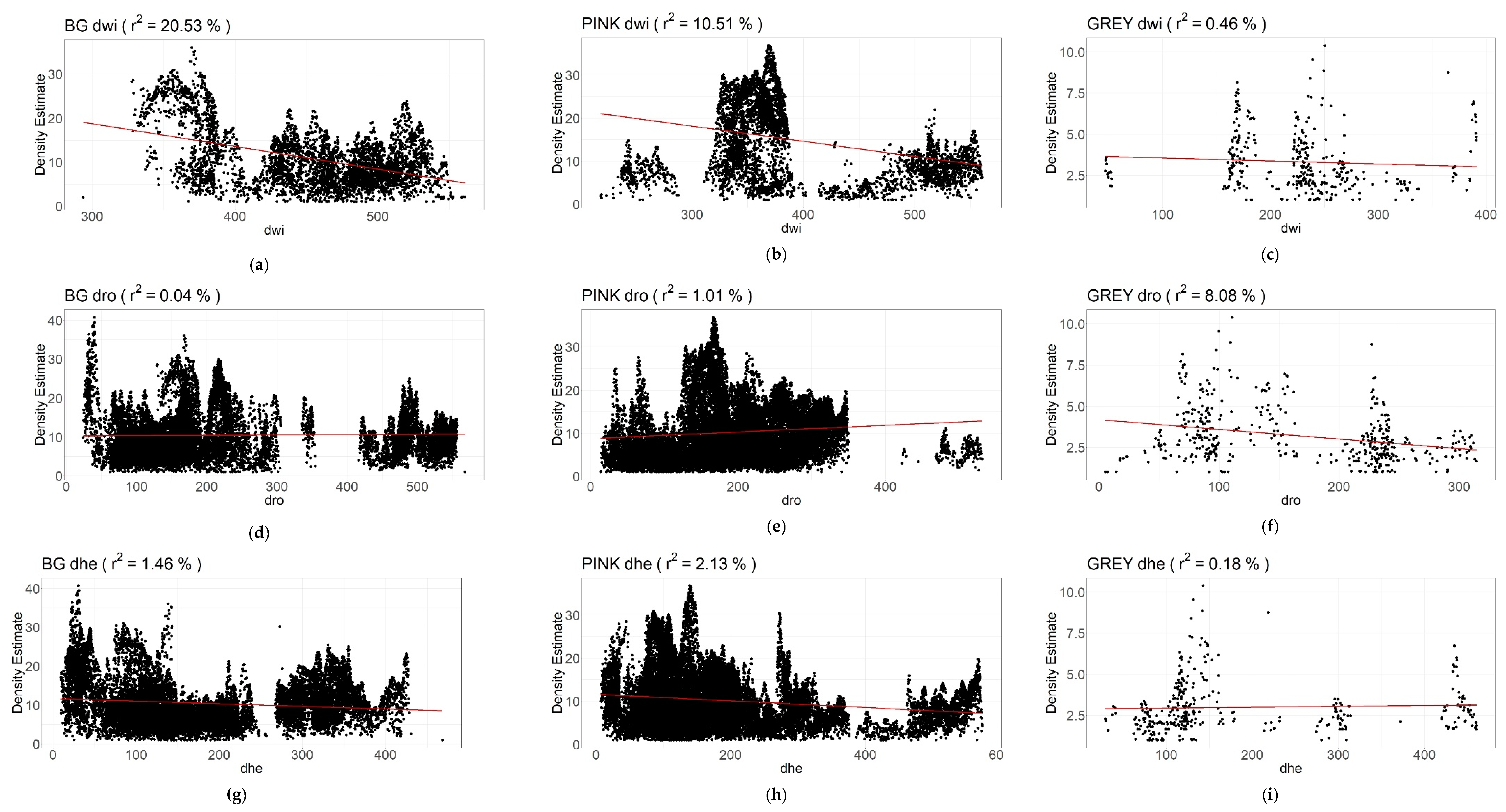
The barnacle geese and pink-footed geese showed a significant increase of BSYM with decreasing distance to the wind turbines (r2 = 20.53%) *** and (r2 = 10.51%) *** respectively (Table 1 and Figure 2a,d). The greylag geese showed the same trend, but the regression was not significant (r2 = 0.45%, p > 0.05) (Table 1 and Figure 2g).

3.1.2. Roads

The greylag geese showed a significant increase of BSYM with decreasing distance to the roads (r2 = 8.08%) *** (Table 1 and Figure 2h). Whereas, barnacle geese and pink-footed geese showed (with r2 < 5%) the opposite trend with a significant decrease of BSYM with decreasing distance to the roads (r2 = 0.04%) *** and (r2 = 1.01%) *** respectively (Table 1 and Figure 2b,e).

3.1.3. Hedgerows

Barnacle geese and pink-footed geese showed a significant (with r2 < 5%) increase of BSYM with decreasing distance to the hedgerows (r2 = 1.46%) *** and (r2 = 2.13%) *** respectively (Table 1 and Figure 2c,f).
The greylag geese showed (with a non-significant regression and r2 < 5%) the opposite trend with a significant decrease of BSYM with decreasing distance to the hedgerows (r2 = 0.18%, p > 0.05) (Table 1 and Figure 2i).

3.2. Correlation between Distance to Landscape Elements and Behavioural Instability of Variance (BVAR)

3.2.1. Wind Turbines

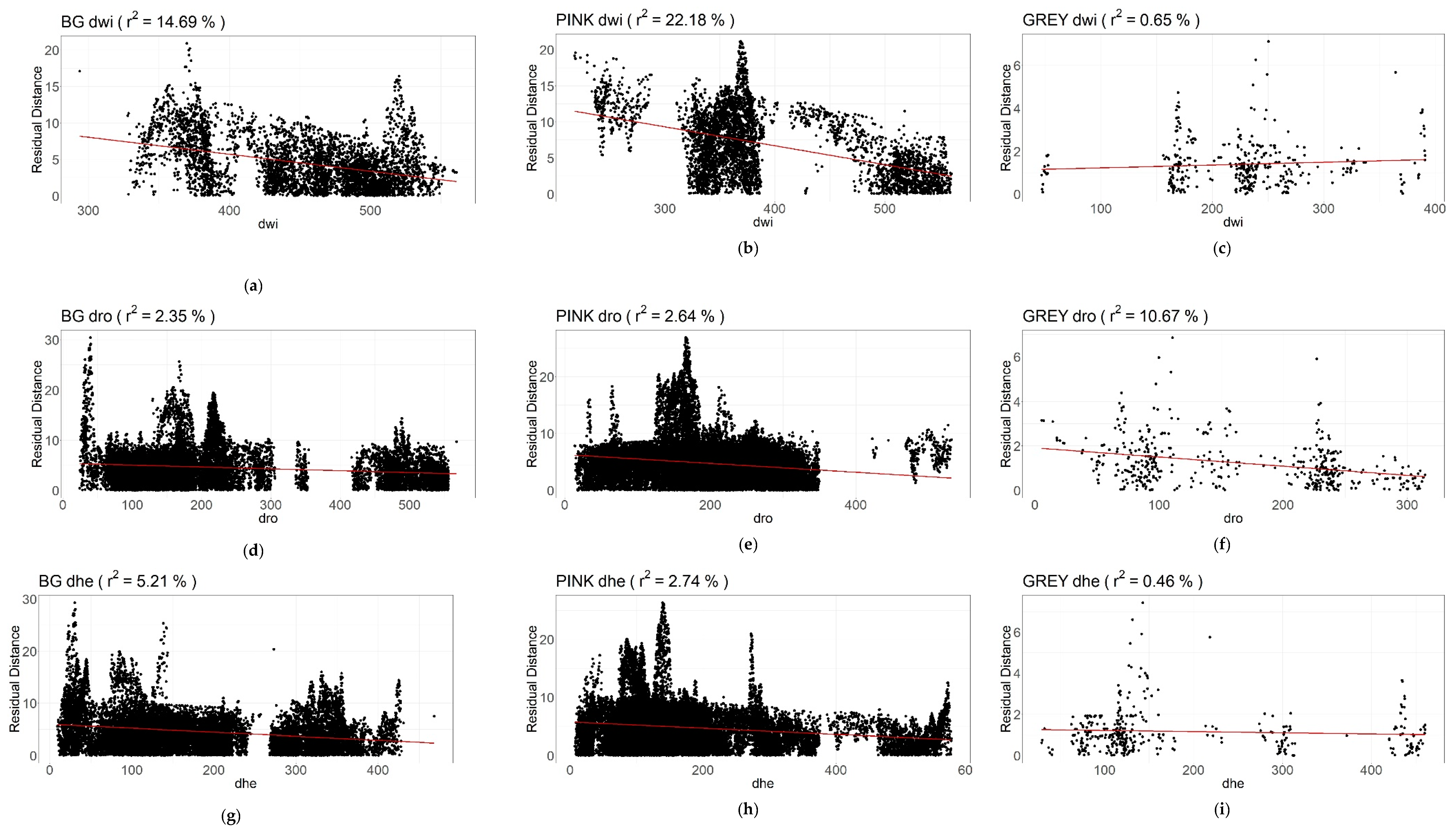
The barnacle geese and pink-footed geese showed a significant increase of BVAR with decreasing distance to the wind turbines (r2 = 14.69%) *** and (r2 = 22.18%) *** respectively (Table 1 and Figure 3a,d). Whereas, the greylag geese showed (with r2 < 5% and p > 0.05) the opposite trend with a decrease of BVAR with decreasing distance to the wind turbines (Table 1 and Figure 3g).

3.2.2. Roads

The greylag geese showed a significant increase of BVAR with decreasing distance to the roads (r2 = 10.67%) *** (Table 1 and Figure 3h). Whereas, barnacle geese and pink-footed geese showed a significant increase (with r2 < 5%) increase of BVAR with decreasing distance to the roads (r2 = 2.35%) *** and (r2 = 2.64%) *** respectively (Table 1 and Figure 3b,e).

3.2.3. Hedgerows

The barnacle geese showed a significant increase of BVAR with decreasing distance to the hedgerows (r2 = 5.20%) ***, (Table 1 and Figure 3c). Whereas, pink-footed geese showed a significant (with r2 < 5%) increase of BVAR with decreasing distance to the hedgerows (r2 = 2.74%) ***, (Table 1 and Figure 3f).
Lastly, the greylag geese showed (with a non-significant regression and r2 < 5%) an increase of BVAR with decreasing distance to the hedgerows (r2 = 0.46%, p > 0.05) ***, (Table 1 and Figure 3f).

4. Discussion

We have shown that the spatial distribution of foraging geese changes when they get closer to a disturbing landscape element (Table 1, Figure 2 and Figure 3) and clear tendencies were observed indicating an increasing anti-predator cohesion of flocks of geese with decreasing distance to disturbing landscape elements. The change in spatial distribution is visible both for the behavioural instability of symmetry (BSYM) and behavioural instability of variance (BVAR), which will be discussed below.
There are clear tendencies, with few exceptions (with r2 < 5%), for negative slopes of the linear regression of density (LRD), which indicates an increasing BSYM with decreasing distance to the landscape elements (Table 1 and Figure 2). There is also a clear tendency with few exceptions (with r2 < 5%) for a negative slope of the linear regression of residuals (LRRs), which means an increasing BVAR with decreasing distance to the landscape elements (Table 1 and Figure 3). Thus, both indices show asymmetry of spatial distribution, implying environmental stress in flocks of geese induced by foraging near the studied landscape elements, which indicates these measurements to be useful tools for monitoring environmental stress. We have chosen the 5% threshold arbitrarily; however, it is also notable that the same negative trends were observed for other LRD and LRR although with r2 below 5% (Figure 2 and Figure 3). However, such relatively weak trends might not be of biological importance and should thus be interpreted with caution. Additionally, p-values also should be evaluated cautiously as the large sample size increases the significance of the indices even with low r2 as seen in both indices (Table 1). These relatively low r2 values might be caused by noise from other factors influencing the density of bird flocks, masking the disturbing effects of the landscape elements. Such factors might include flock size [11] as well as food and water distribution [12], which are both known to affect the density and spatial distribution of bird flocks. Especially BVAR might have been affected by variations in flock size as flocks of different size prioritise anti-predation behaviour and foraging beneficial behaviour differently. A study by Lazarus [11], who examined the influence of flock size on the vigilance of white-fronted geese (Anser albifrons), noted that the percentage of vigilant birds in a flock would decrease steeply at flock sizes above 200–300 individuals [11]. Hence, larger flocks might prioritise foraging beneficial behaviour while smaller flocks prioritise anti-predator behaviour through the dilution effect [7,11,13,14]. However, trends were still observed for both BSYM and BVAR that prove that both methods can be applied to wildlife behaviour with multiple random influences, as long as the factor of interest is measured across a correlated variable.
In our study linear relationships were assumed and therefore only linear regression has been utilized. However, BSYM and BVAR could also be applied in studies with a non-linear relationship between the independent value and the dependent value. In this case, the asymmetry on the left and right side of mean can vary and might be estimated by the first derivative, which is equivalent to the slope observed for a certain value of the dependent value. Therefore, the BSYM index can be considered the equivalent of the absolute values of the difference between right and left value of a trait, which was referred to as fluctuating asymmetry (FA1) [15] in a study by Palmer and Strobeck [15]. Whereas, BVAR indices can be considered the equivalent of the phenotypic variability of trait (Vp). For both indices, FA1 and Vp are often utilised as estimators of developmental instability (DI) [16].

5. Conclusions

We have tested both indices against distance to landscape elements as an independent variable; however, the indices could also be utilised for other possible variables, e.g., regression against time or temperature. The merit of BSYM and BVAR is that they do not need bilateral traits for the estimation of the instability, which in our case we have called behavioural instability as we are estimating a deviation from expected behaviour, which is a constant distance between every single individual due to a uniform distribution of the individuals. These indices have proven effective tools for assessing the effect of environmental stress on expected behaviour. Thus, the term behavioural instability has been proven useful for data other than bilateral data as discussed in Pertoldi et al. [1]. We expect that the application of these two indices BSYM and BVAR could have several applications in applied ecology as both indices can be regressed against environmental gradients or temporal series.

Author Contributions

M.B.-H., R.M.K. and C.P. conceptualised the project and did the methodology. C.P. provided the resources, while M.B.-H., R.M.K., J.H.F.C. and J.B.G. did the investigation and data curation. M.B.-H., R.M.K., D.B., J.B.G. and C.P. did the formal analysis and visualization. M.B.-H., R.M.K. and C.P. took the lead in writing the manuscript. All authors provided critical feedback and helped shape the research, analysis and manuscript. M.B.-H. and R.M.K. were responsible for the project administration as well as, research activities and planning, who were supervised by D.B., B.L., L.F.J. and C.P.

Funding

Mads Bech-Hansen, Rune M. Kallehauge and Cino Pertoldi were financed by the Aalborg Zoo Conservation Foundation (AZCF: grant number 2018-4).

Acknowledgments

We would like to thank the Lead Guest Editor and the anonymous reviewers for invaluable suggestions and comments on the manuscript.

Conflicts of Interest

The authors declare no conflict of interest.

References

  1. Pertoldi, C.; Bahrndorff, S.; Novicic, Z.K.; Rohde, P.D. The Novel Concept of “Behavioural Instability” and Its Potential Applications. Symmetry 2016, 8, 135. [Google Scholar] [CrossRef]
  2. Rees, E.C. Impacts of wind farms on swans and geese: A review. Wildfowl 2012, 62, 37–72. [Google Scholar]
  3. Madsen, J. Impact of Disturbance on Field Utilization of Pink-footed Geese in West Jutland, Denmark. Biol. Conserv. 1985, 33, 53–63. [Google Scholar] [CrossRef]
  4. Larsen, J.K.; Madsen, J. Effects of wind turbines and other physical elements on field utilization by pink-footed geese (Anser brachyrhynchus): A landscape perspective. Landsc. Ecol. 2000, 15, 755–764. [Google Scholar] [CrossRef]
  5. Chudziǹska, M.E.; van Best, F.M.; Madsen, J.; Nabe-Nielsen, J. Using habitat selection theories to predict the spatiotemporal distribution of migratory birds during stopover—A case study of pink-footed geese Anser brachyrhynchus. Oikos 2015, 124, 854–860. [Google Scholar] [CrossRef]
  6. Harrison, A.L.; Petkov, N.; Mitev, D.; Popgeorgiev, G.; Gove, B.; Hilton, G.M. Scale-dependent habitat selection by wintering geese: Implications for landscape management. Biodivers. Conserv. 2018, 27, 167–188. [Google Scholar] [CrossRef]
  7. Hötker, H. Birds: Displacement. In Wildlife and Wind Farms, Conflicts and Solutions; Volume 1 Onshore: Potential Effects; Perrow, M.R., Ed.; Pelagic Publishing: Exeter, UK, 2017; pp. 119–154. [Google Scholar]
  8. Roberts, G. Why individual vigilance declines as group size increases. Anim. Behav. 1996, 51, 1077–1086. [Google Scholar] [CrossRef] [Green Version]
  9. Bech-Hansen, M.; Kallehauge, R.M.; Lauritzen, J.M.S.; Sørensen, M.H.; Pertoldi, C.; Bruhn, D.; Laubek, B.; Jensen, L.F. Evaluation of disturbance effect on geese and swans (Anserinae) caused by an approaching unmanned aerial vehicle. Bird Conserv. Int. under review.
  10. Silverman, B. Density Estimation for Statistics and Data Analysis; Chapman & Hall: London, UK, 1986; pp. 9–13. [Google Scholar]
  11. Lazarus, J. Vigilance, flock size and domain of danger size in the White-fronted Goose. Wildfowl 1978, 29, 135–145. [Google Scholar]
  12. Gill, J.A. Habitat Choice in Pink-Footed Geese: Quantifying the Constraints Determining Winter Site Use. J. Appl. Ecol. 1996, 33, 884–892. [Google Scholar] [CrossRef]
  13. Black, M.J.; Carbone, C.; Wells, R.L.; Owen, M. Foraging dynamics in goose flocks: The cost of living on the edge. Anim. Behav. 1992, 44, 41–50. [Google Scholar] [CrossRef]
  14. Carbone, C.; Thompson, W.A.; Zadorina, L.; Rowcliffe, J.M. Competition, predation risk and patterns of flock expansion in barnacle geese (Branta leucopsis). J. Zool. Lond. 2003, 259, 301–308. [Google Scholar] [CrossRef]
  15. Palmer, A.R.; Strobeck, C. Fluctuating asymmetry: Measurement, analysis, patterns. Annu. Rev. Ecol. Syst. 1986, 17, 391–421. [Google Scholar] [CrossRef]
  16. Pertoldi, C.; Kristensen, T.N.; Andersen, D.H.; Loeschcke, V. Developmental instability as an estimator of genetic stress. Heredity 2006, 96, 122–127. [Google Scholar] [CrossRef] [PubMed]
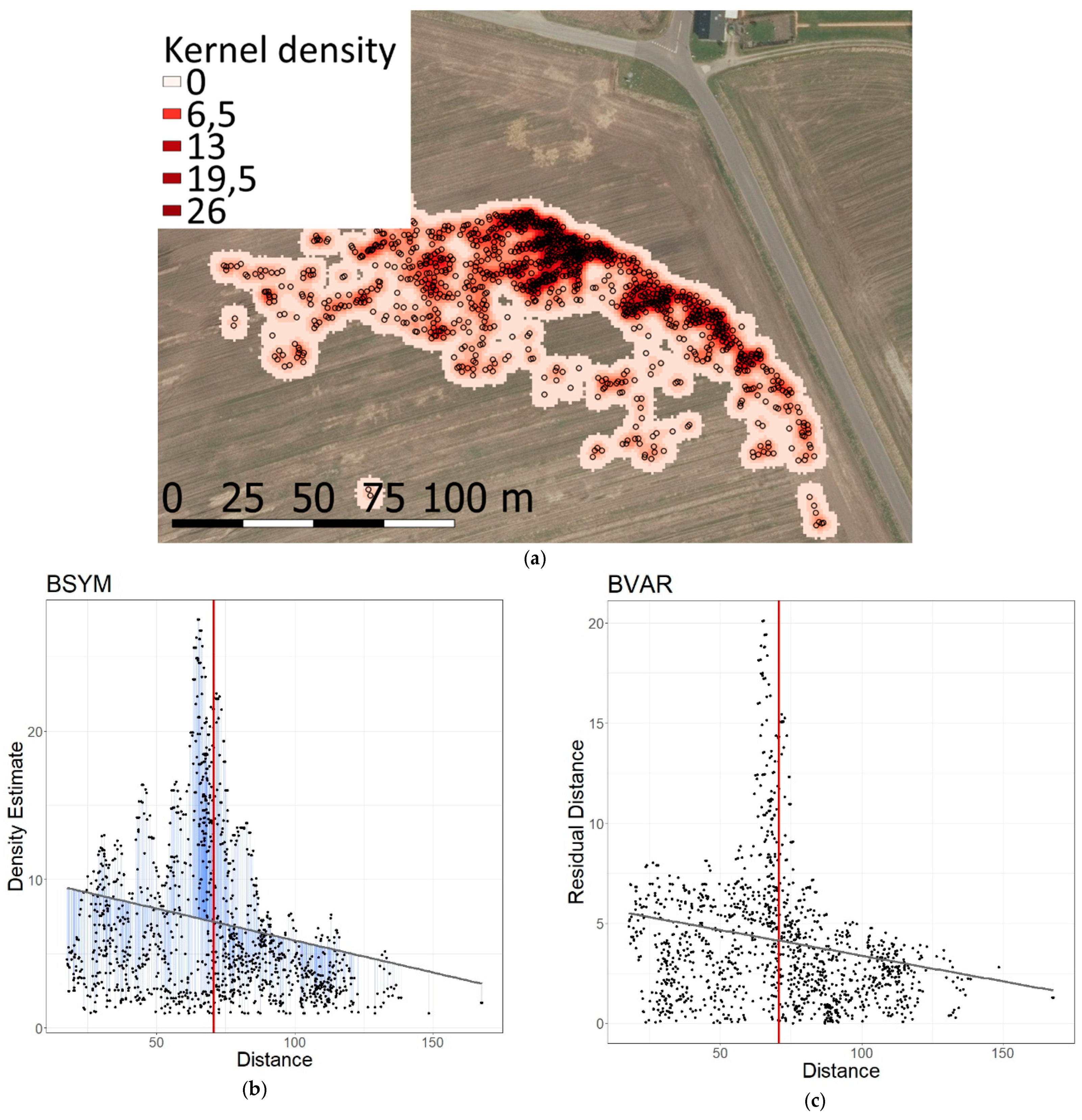
Figure 1. Overview of behavioural instability indices used to monitor one flock of pink-footed geese foraging near a road: (a) Aerial photos of a flock of individual geese are georeferenced in geographic information systems (GIS) and geographic positions of individual geese are geotagged (illustrated as circles). Flock density is quantified by Kernel density estimates using the geographic positions of identified birds. Kernel density estimates are illustrated as white (low density) to dark red (high density); (b) Density estimates of individuals as a function of distance to the nearest landscape element, in this case, roads. The mean distance is illustrated as a red vertical line. A linear regression of density (LRD): Density Estimate = a × Distance + b (illustrated as a grey line) is fitted to measure behavioural instability through asymmetry of density between distances left and right of the mean distance. Symmetrical density would result in a non-significant slope (a = 0). Contrarily, an anti-predator behaviour induced by the road would yield a negative slope (a < 0). Residual distances between observed densities and LRD is illustrated as blue lines; (c) Residual distances of density (Figure 1b) as a function of distance to the nearest landscape elements, in this case roads. A linear regression of residuals (LRR): Residual = a × Distance + b (illustrated as a grey line) is fitted to measure behavioural instability through asymmetry of variance in density between distances left and right of the mean distance. A constant variance in density across distance would result in a non-significant slope (a = 0). Contrarily, increased variance would yield a negative slope (a < 0).
Symmetry 11 01103 g001
Figure 2. Linear regression of density (LRD) (illustrated as a red line), which regresses the density estimates of individual birds as a function of bird distances to the nearest landscape element. The following species were regressed: barnacle goose (BG), pink-footed goose (PINK), and Greylag goose (GREY). Distances from the landscape elements: wind turbines (dwi), roads (dro), and hedgerows (dhe). The r2 values of LRD above 5% (r2 > 5%) are in bold.
Symmetry 11 01103 g002
Figure 3. Linear regression of residuals (LRR) (illustrated as a red line), which regresses the absolute values of the residuals from LRD were regressed as a function of bird distances to the nearest landscape element. The following species were regressed: barnacle goose (BG), pink-footed goose (PINK), and greylag goose (GREY). Distances from the landscape elements; wind turbines (dwi), roads (dro), and hedgerows (dhe). The r2 values of LRR above 5% (r2 > 5%) are in bold.
Symmetry 11 01103 g003
Table 1. Species: Barnacle goose (BG), pink-footed goose (PINK), and greylag goose (GREY); distances from the landscape elements: wind turbines (dwi), roads (dro), and hedgerows (dhe), n = number of measurements. Coefficient of determination (r2) slope (a), intercept (b) and significance level (p) of both linear regression of density (LRD) (which regress the density estimates of individual birds as a function of bird distances to nearest landscape element) and of linear regression of residuals (LRR) (which regress the absolute values of residual distance from LRD as a function of bird distances to nearest landscape element). The r2 values above 5% (r2 > 5%) are in bold.
Species Dist. from Obstaclesn (Number of Measurements)LRD r2LRD a & bLRD pLRR r2LRR a & bLRR p
BGdwi487220.53%Slope a:
Intercept b:
−0.052
34.182
***14.69%Slope a:
Intercept b:
−0.023
15.038
***
dro189250.04%Slope a:
Intercept b:
0.001
10.258
**2.35%Slope a:
Intercept b:
−0.004
5.394
**
dhe189251.46%Slope a:
Intercept b:
−0.007
11.610
***5.20%Slope a:
Intercept b:
−0.008
5.968
***
PINKdwi489410.51%Slope a:
Intercept b:
−0.035
28.681
***22.18%Slope a:
Intercept b:
−0.026
17.196
***
dro263941.01%Slope a:
Intercept b:
−0.008
8.744
***2.64%Slope a:
Intercept b:
−0.008
6.301
***
dhe263132.13%Slope a:
Intercept b:
0.008
11.588
***2.74%Slope a:
Intercept b:
−0.005
5.734
***
GREYdwi3610.45%Slope a:
Intercept b:
−0.002
3.720
n.s.0.65%Slope a:
Intercept b:
0.001
1.090
n.s.
dro4588.08%Slope a:
Intercept b:
−0.006
4.176
***10.67%Slope a:
Intercept b:
−0.004
1.910
***
dhe3530.18Slope a:
Intercept b:
0.001
2.873
n.s.0.46%Slope a:
Intercept b:
−0.001
1.22
n.s.
p < 0,05 = *, p < 0,01 = **, p < 0.0001 = ***, and n.s. = non-significant.