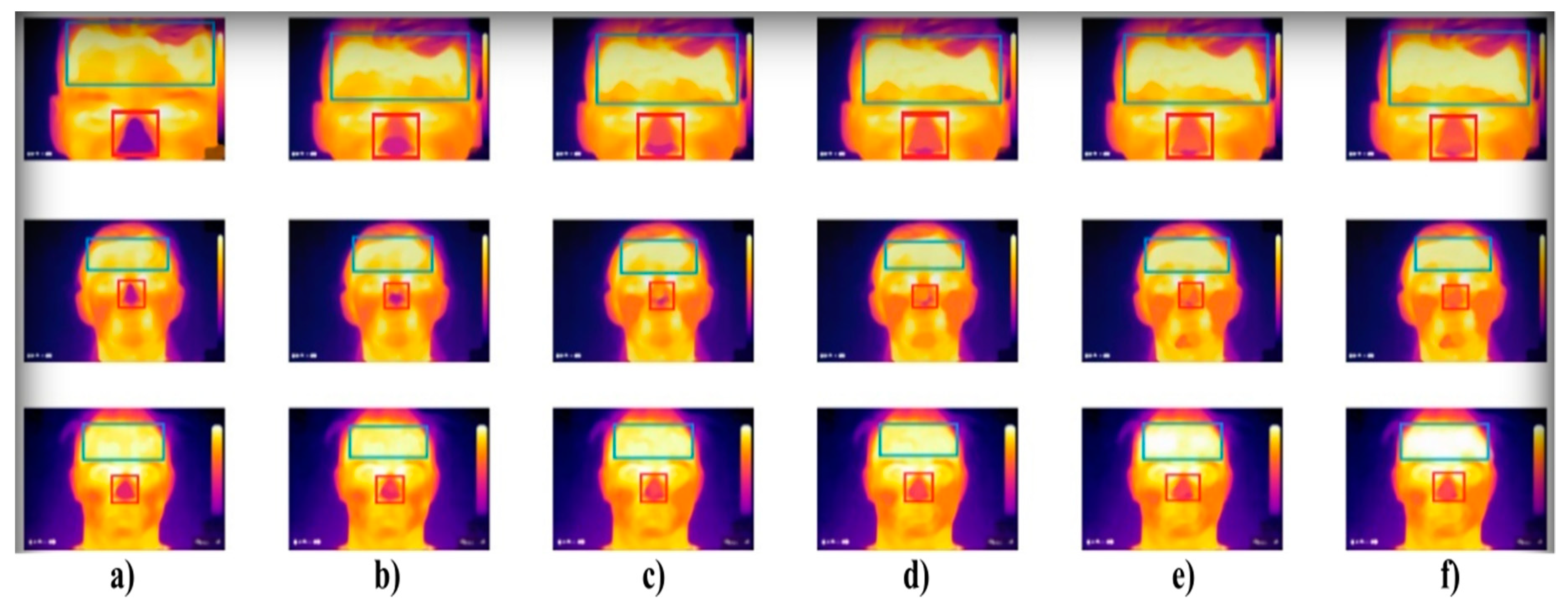
Figure 1.
Extract of the IR measurement of three individuals (rows) where: (a) sober state, (b) 40 mL, (c) 80 mL, (d) 120 mL, (e) 160 mL, and (f) 200 mL of alcohol. The forehead and nose were detected by using the Viola–Jones object detection to indicate individual facial areas. The hottest area of the forehead is getting expanded, while the coldest area of the nose is getting reduced within alcohol intoxication.
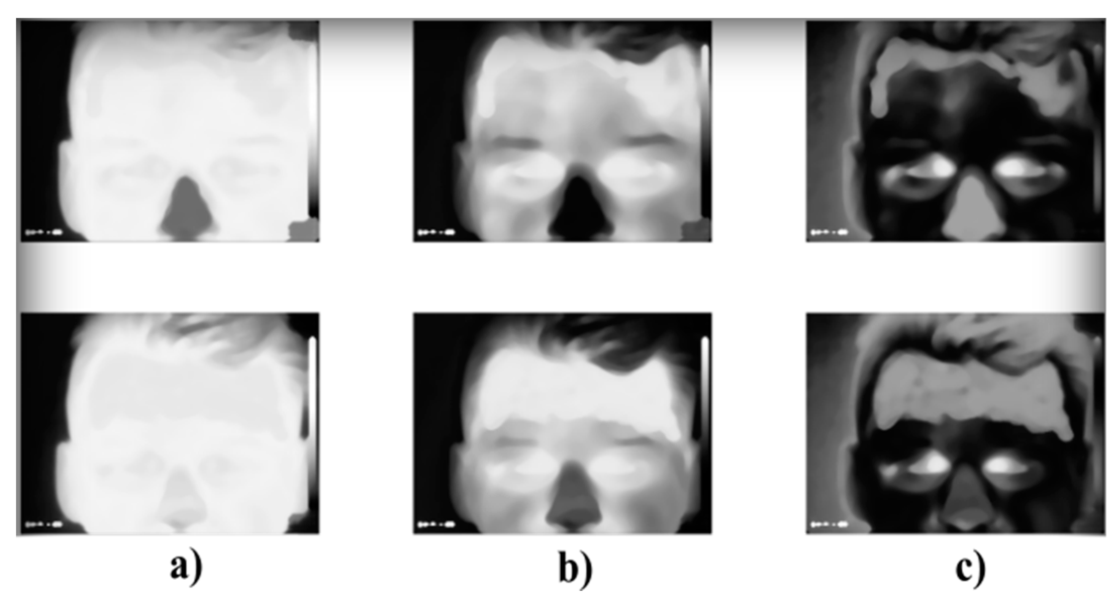
Figure 2.
Comparison of the RGB decomposition for sober state (top row) and after 200 mL of 38% alcohol (down row), where: (a) R layer, (b) G layer, and (c) B layer.
Figure 2.
Comparison of the RGB decomposition for sober state (top row) and after 200 mL of 38% alcohol (down row), where: (a) R layer, (b) G layer, and (c) B layer.
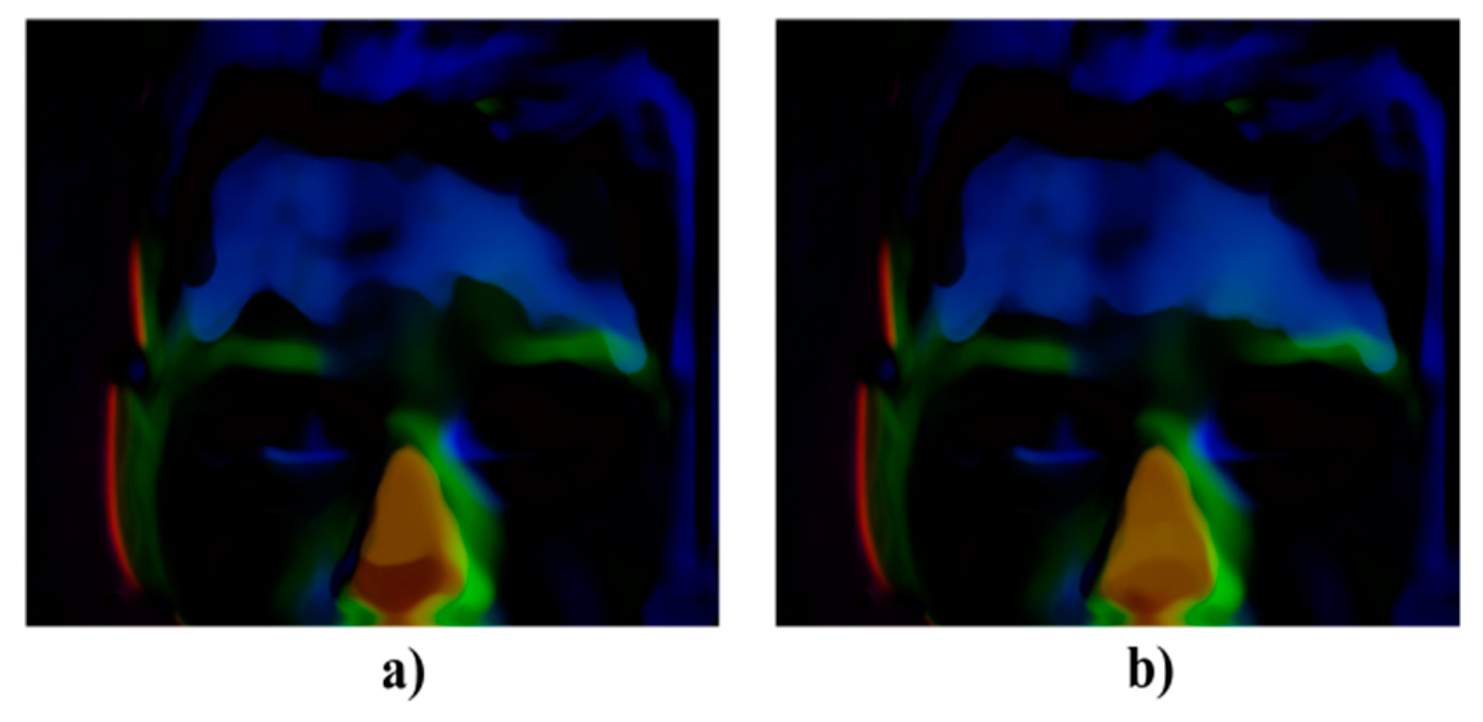
Figure 3.
Showing differences of the IR image taken after (a) 100 mL of the alcohol and (b) 200 mL of alcohol against the sober state.
Figure 3.
Showing differences of the IR image taken after (a) 100 mL of the alcohol and (b) 200 mL of alcohol against the sober state.
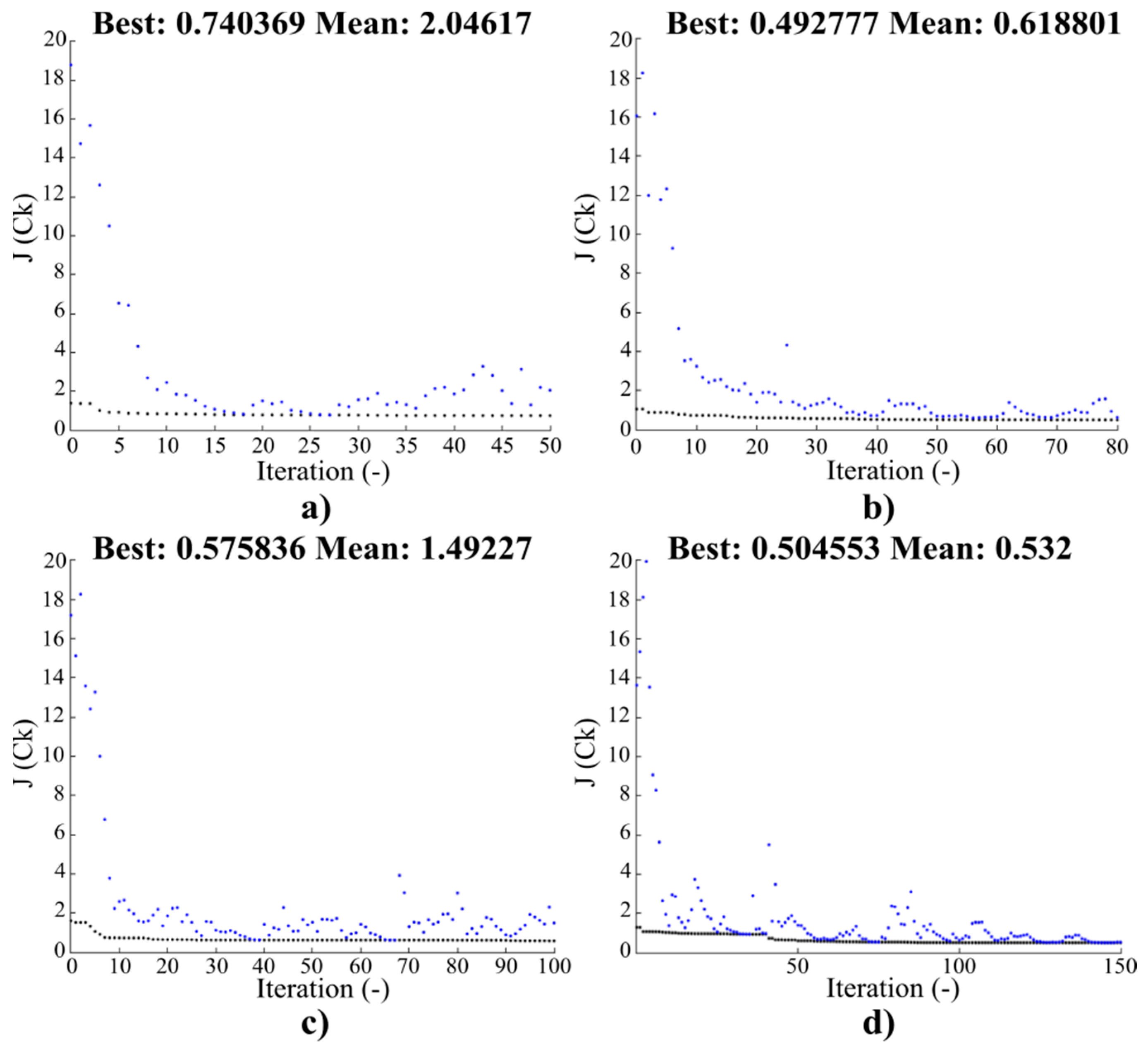
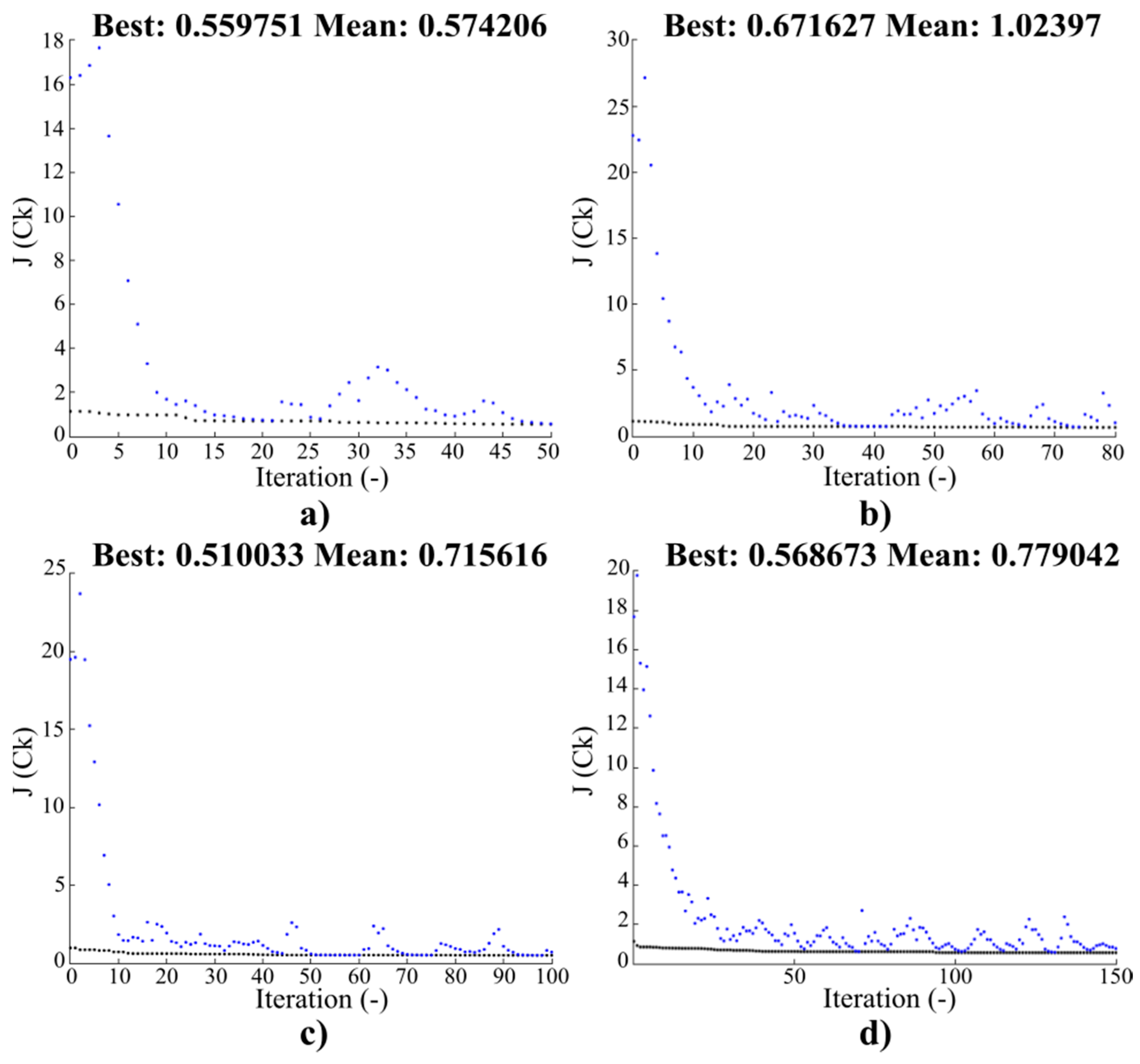
Figure 4.
Convergence characteristics for the objective function J(Ck) for the initial population SN = 80: (a) 50, (b) 80, (c) 100, and (d) 150 iterations.
Figure 4.
Convergence characteristics for the objective function J(Ck) for the initial population SN = 80: (a) 50, (b) 80, (c) 100, and (d) 150 iterations.
Figure 5.
Convergence characteristics for the objective function J(Ck) for the initial population SN = 200: (a) 50, (b) 80, (c) 100, and (d) 150 iterations.
Figure 5.
Convergence characteristics for the objective function J(Ck) for the initial population SN = 200: (a) 50, (b) 80, (c) 100, and (d) 150 iterations.
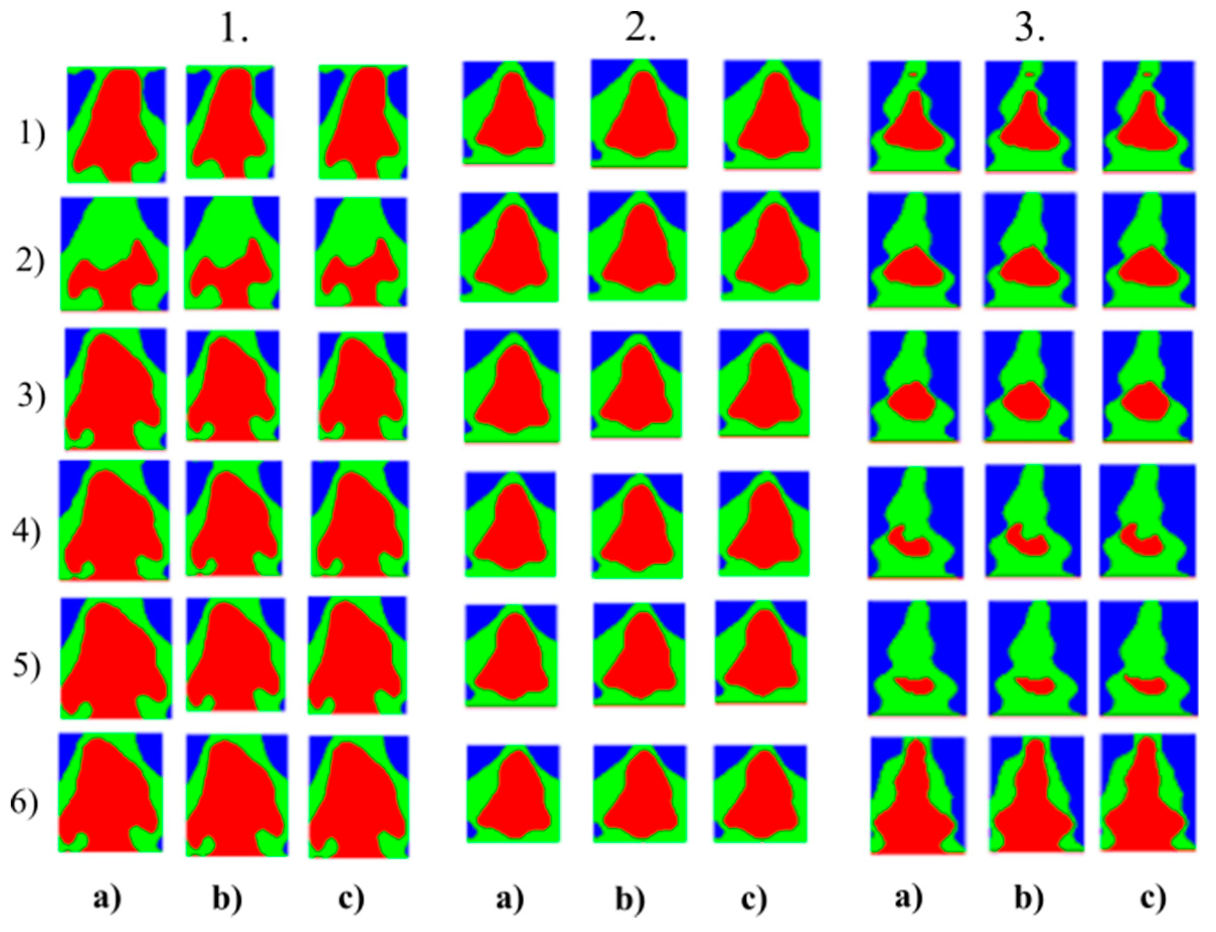
Figure 6.
Multiregional segmentation with three clusters of the nose area for three tested persons for: (a) SN = 100, It = 100, (b) SN = 70, It = 90 and (c) SN = 120, It = 160. From the top, each row corresponds with gradual intoxication: (1) sober state, (2) 40 mL, (3) 80 mL, (4) 120 mL, (5) 160 mL, and (6) 200 mL.
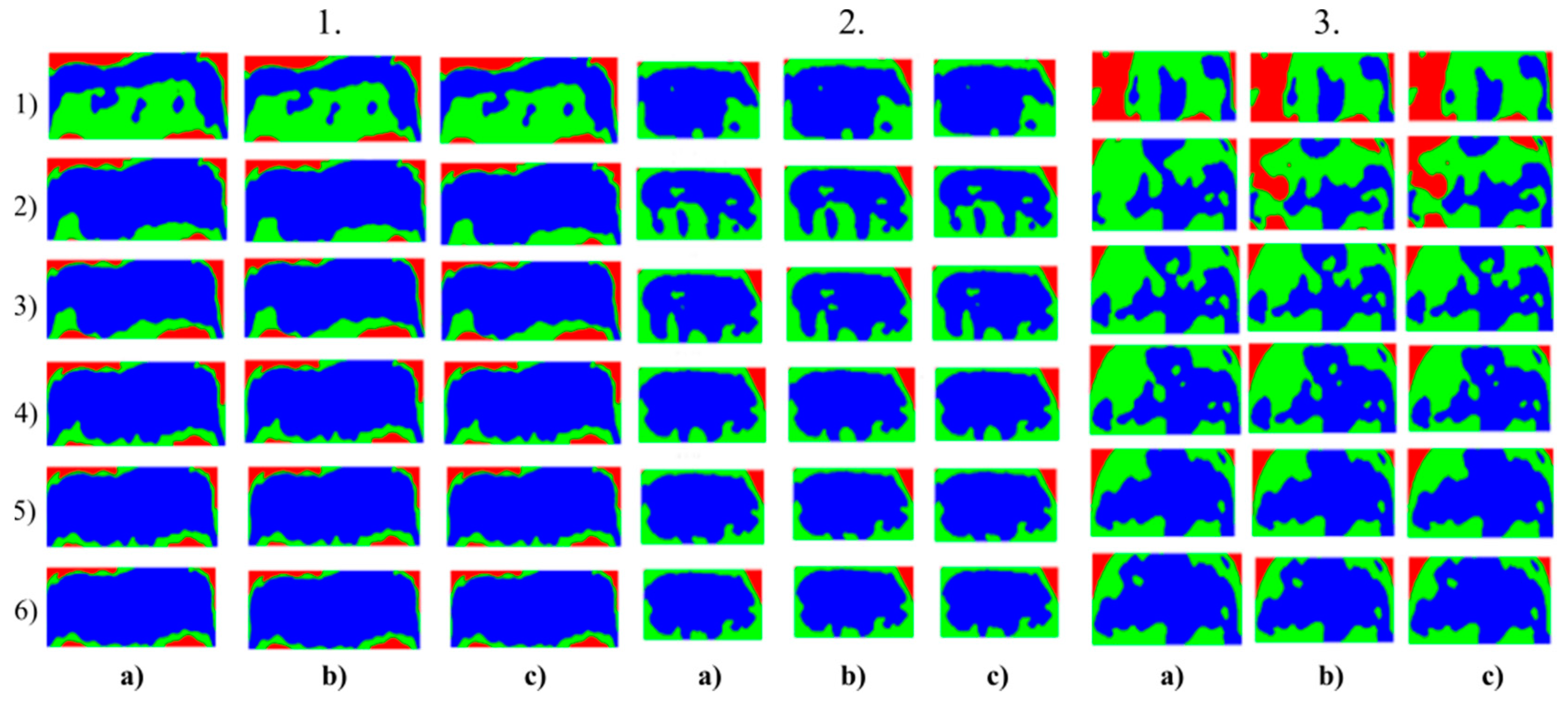
Figure 7.
Multiregional segmentation with three clusters of the forehead area for three tested persons for: (a) SN = 100, It = 100, (b) SN = 70, It = 90, and (c) SN = 120, It = 160. From the top, each row corresponds with gradual intoxication: (1) sober state, (2) 40 mL, (3) 80 mL, (4) 120 mL, (5) 160 mL, and (6) 200 mL.
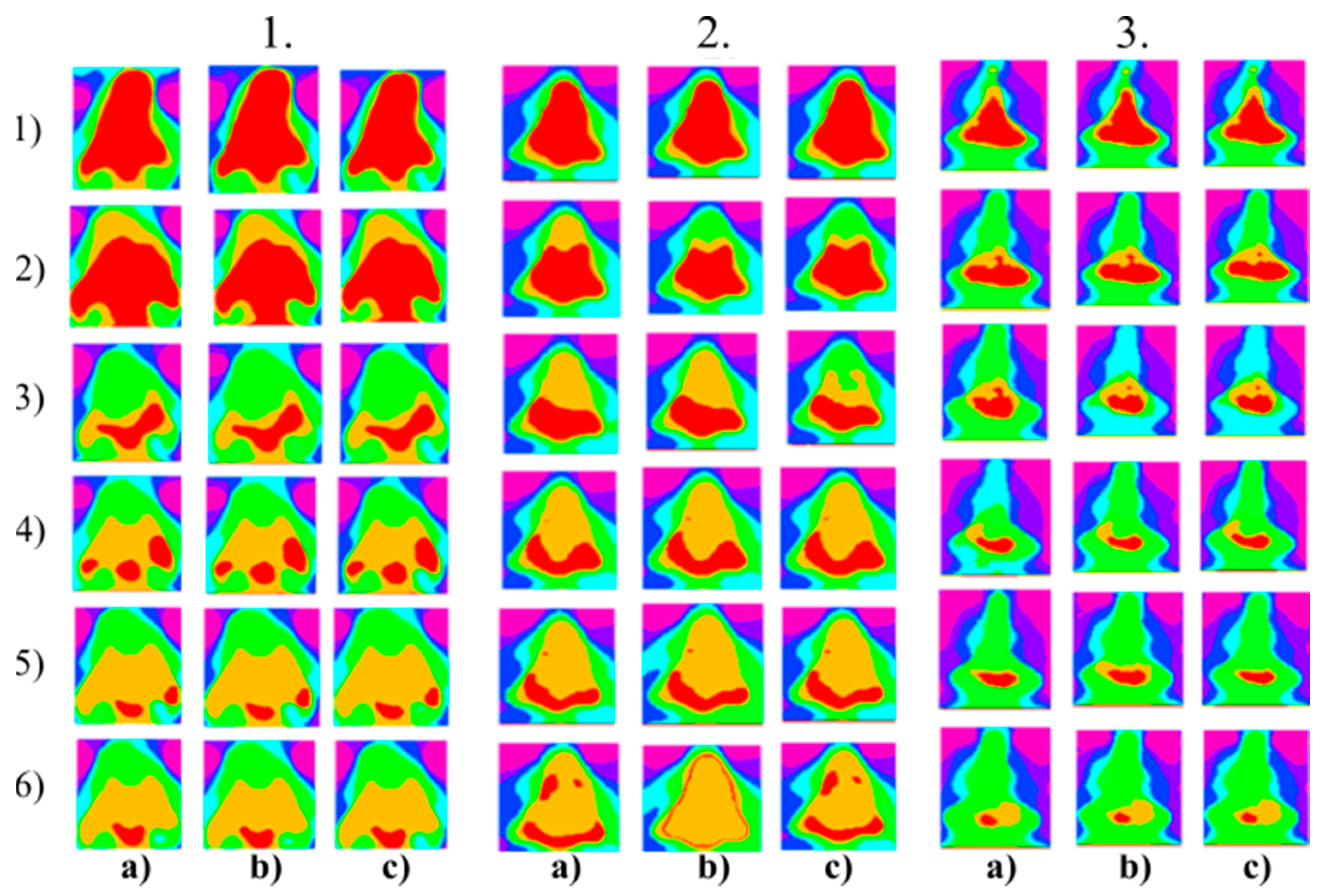
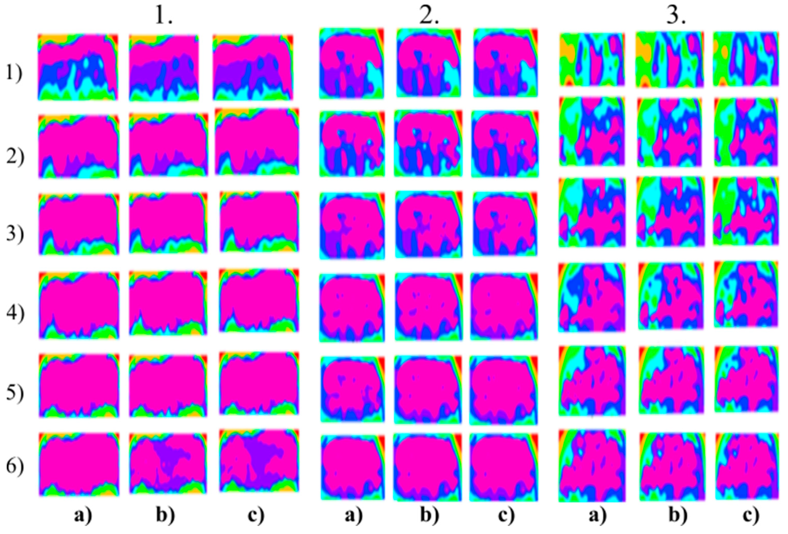
Figure 8.
Multiregional segmentation with eight clusters of the nose area for three tested persons for: (a) SN = 100, It = 100, (b) SN = 70, It = 90 and (c) SN = 120, It = 160. From the top, each row corresponds with gradual intoxication: (1) Sober state, (2) 40 mL, (3) 80 mL, (4) 120 mL, (5) 160 mL, and (6) 200 mL.
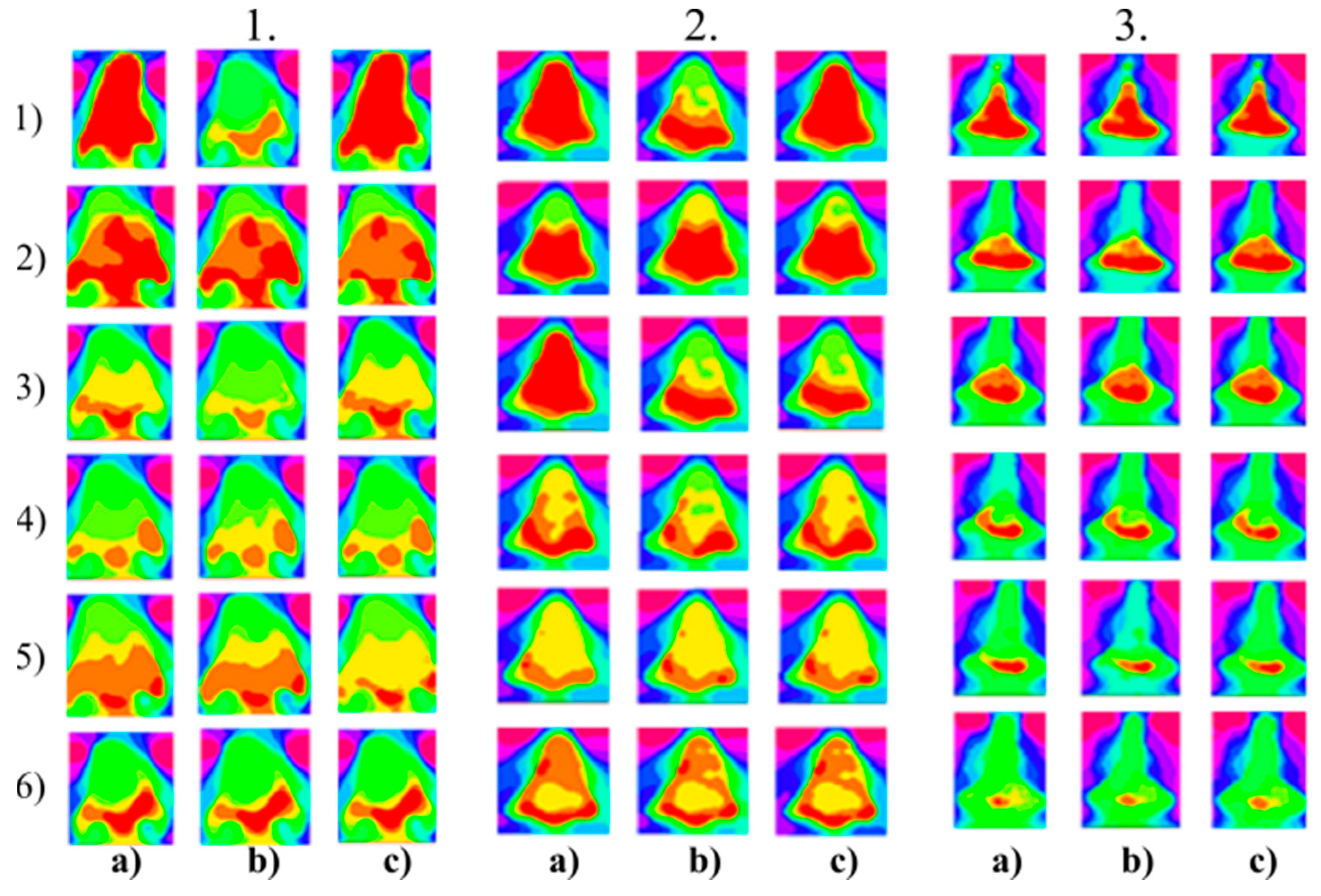
Figure 9.
Multiregional segmentation with eight clusters of the forehead area for three tested persons for: (a) SN = 100, It = 100, (b) SN = 70, It = 90, and (c) SN = 120, It = 160. From the top, each row corresponds with gradual intoxication: (1) sober state, (2) 40 mL, (3) 80 mL, (4) 120 mL, (5) 160 mL, and (6) 200 mL.
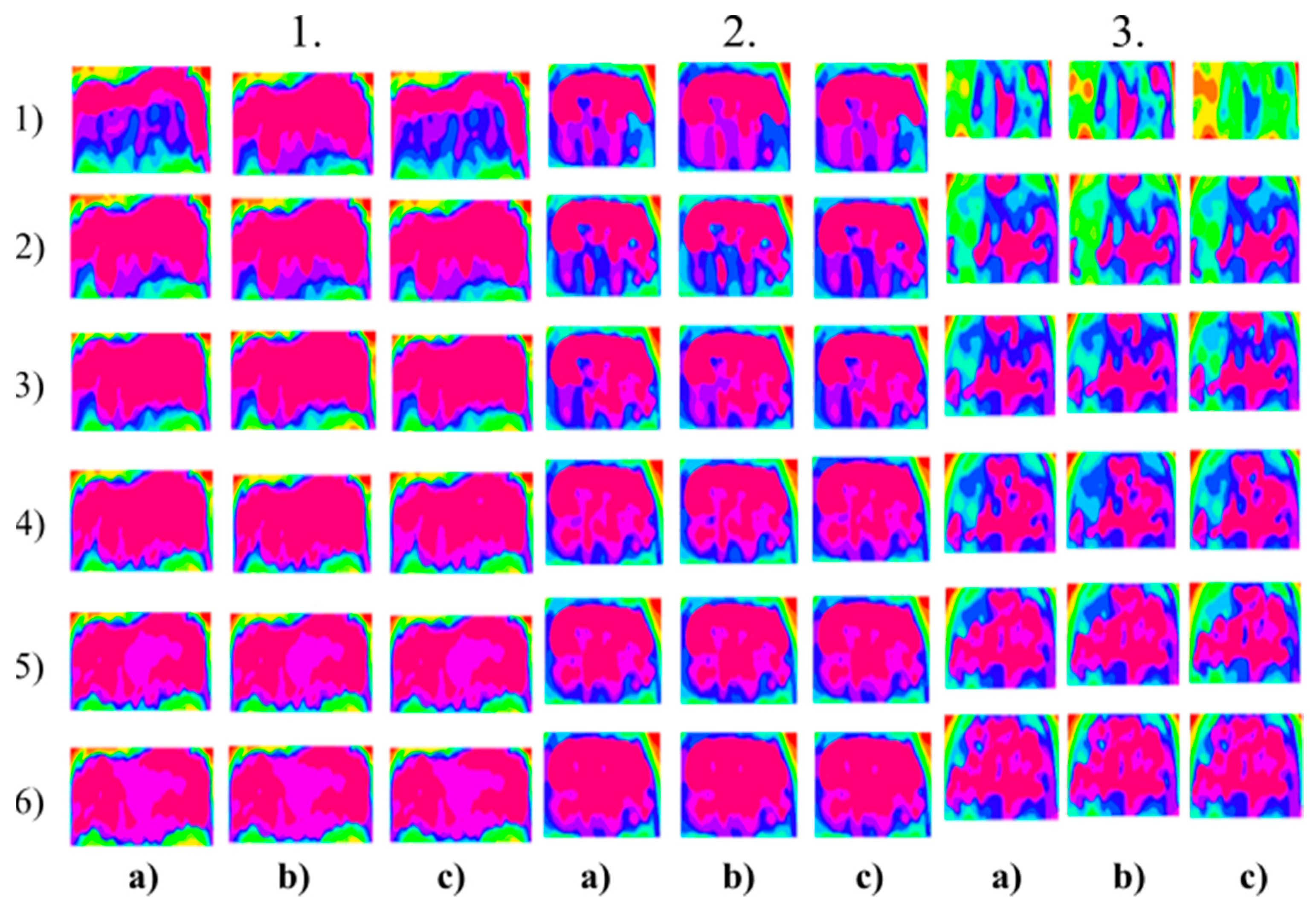
Figure 10.
Multiregional segmentation with eleven clusters of the nose area for three tested persons for: (a) SN = 100, It = 100, (b) SN = 70, It = 90, and (c) SN = 120, It = 160. From the top, each row corresponds with gradual intoxication: (1) sober state, (2) 40 mL, (3) 80 mL, (4) 120 mL, (5) 160 mL, and (6) 200 mL.
Figure 11.
Multiregional segmentation with eleven clusters of the forehead area for three tested persons for: (a) SN = 100, It = 100, (b) SN = 70, It = 90, and (c) SN = 120, It = 160. From the top, each row corresponds with gradual intoxication: (1) sober state, (2) 40 mL, (3) 80 mL, (4) 120 mL, (5) 160 mL, and (6) 200 mL.
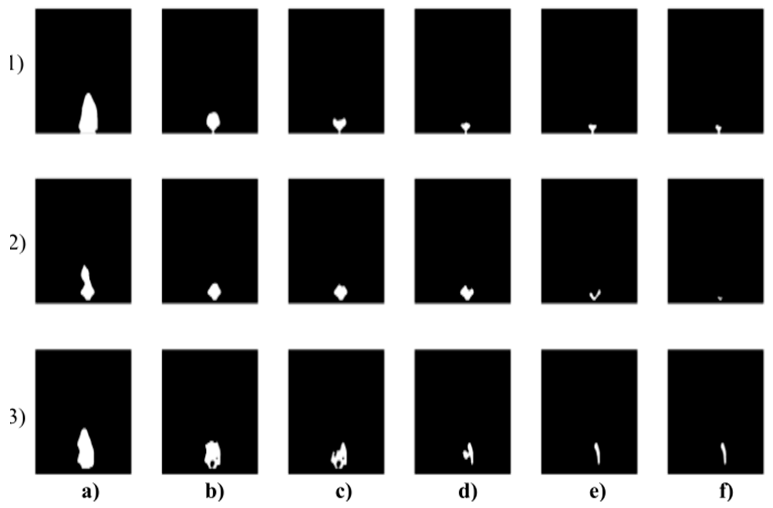
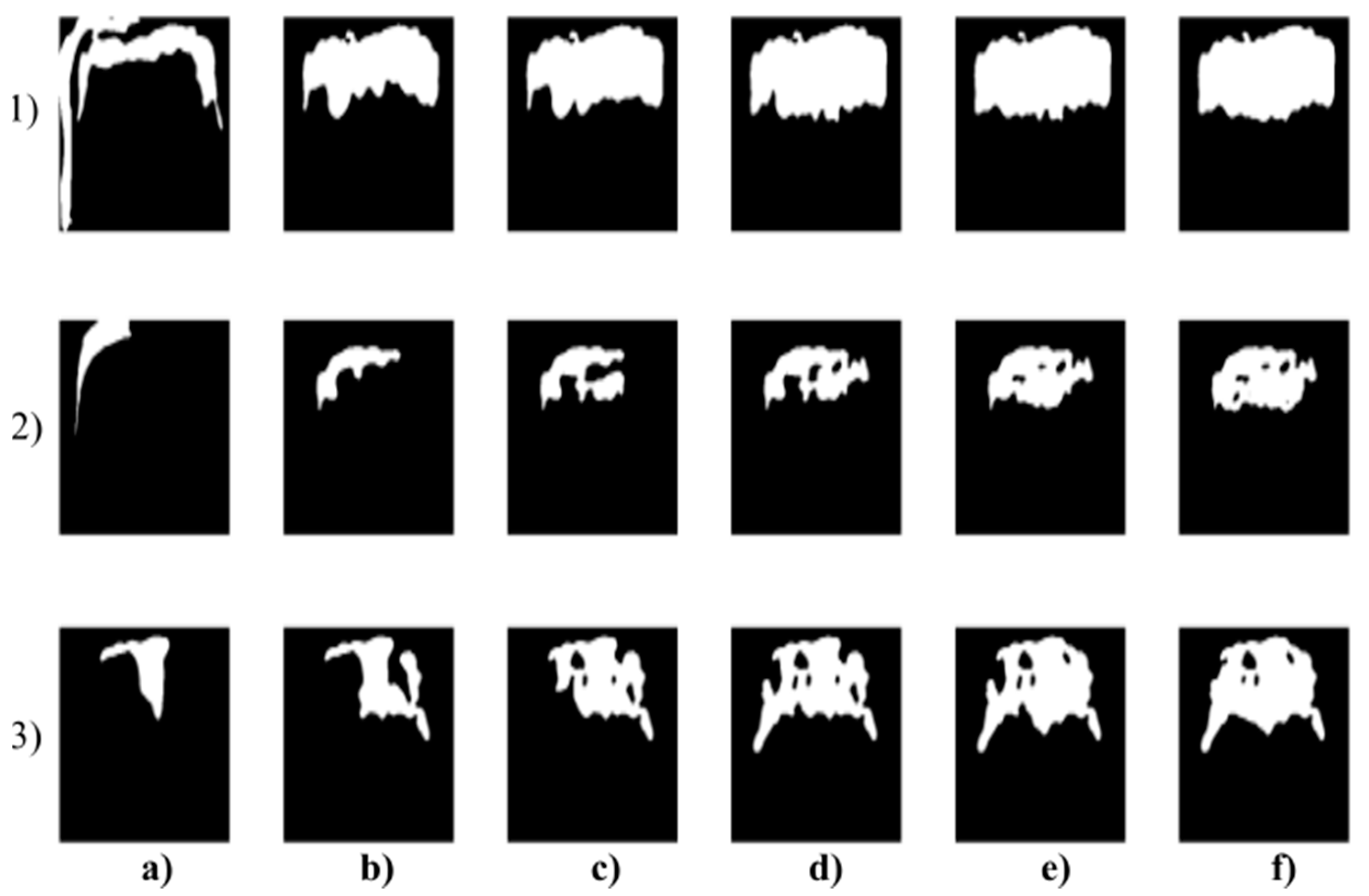
Figure 12.
Binary modeling of the nose dynamical features for three persons (rows) where each column represents gradual alcohol intoxication: (a) Sober state, (b) 40 mL, (c) 80 mL, (d) 120 mL, (e) 160 mL, and (f) 200 mL of the alcohol.
Figure 12.
Binary modeling of the nose dynamical features for three persons (rows) where each column represents gradual alcohol intoxication: (a) Sober state, (b) 40 mL, (c) 80 mL, (d) 120 mL, (e) 160 mL, and (f) 200 mL of the alcohol.
Figure 13.
Binary modeling of the forehead dynamical features for three persons (rows) where each column represents gradual alcohol intoxication: (a) Sober state, (b) 40 mL, (c) 80 mL, (d) 120 mL, (e) 160 mL, and (f) 200 mL of the alcohol.
Figure 13.
Binary modeling of the forehead dynamical features for three persons (rows) where each column represents gradual alcohol intoxication: (a) Sober state, (b) 40 mL, (c) 80 mL, (d) 120 mL, (e) 160 mL, and (f) 200 mL of the alcohol.
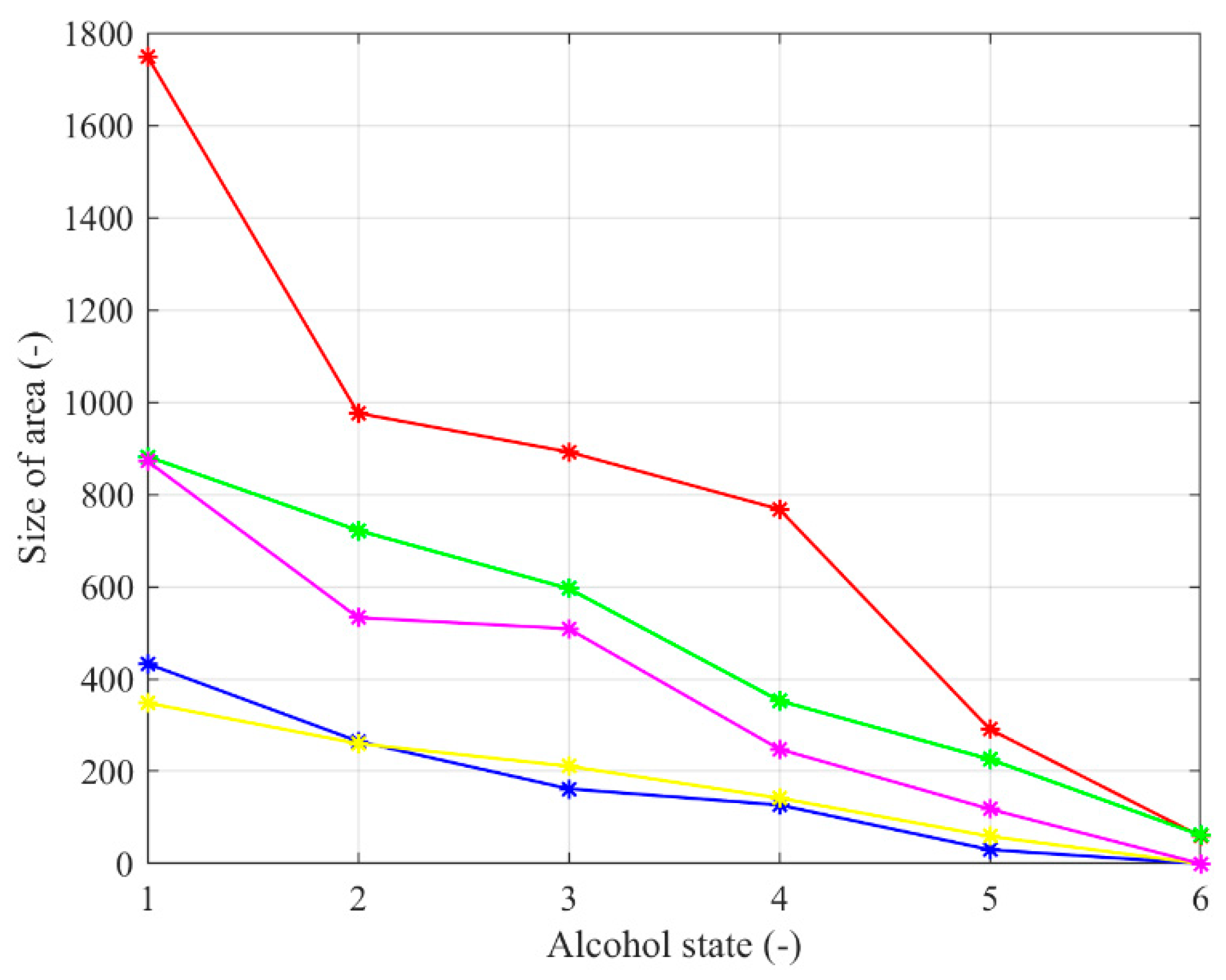
Figure 14.
Averaged decreasing trend of the binary model size for the nose area of 5 tested persons.
Figure 14.
Averaged decreasing trend of the binary model size for the nose area of 5 tested persons.
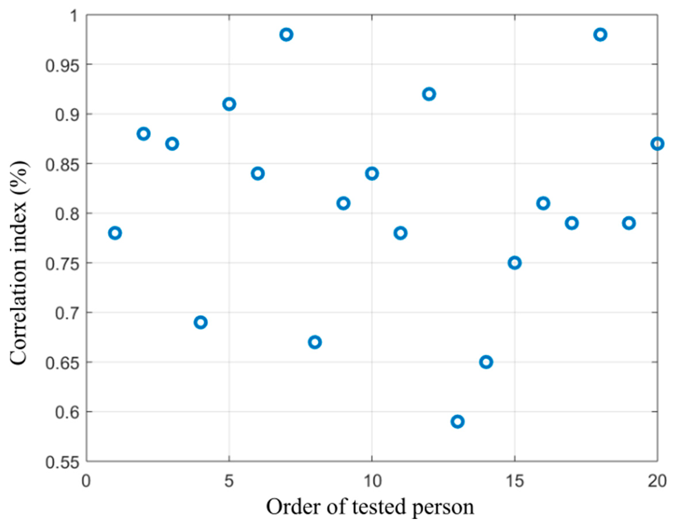
Figure 15.
Distribution of correlation index showing dependency between the alcohol content measured from the breath and area size of the hottest area in the forehead calculated from the proposed segmentation model.
Figure 15.
Distribution of correlation index showing dependency between the alcohol content measured from the breath and area size of the hottest area in the forehead calculated from the proposed segmentation model.
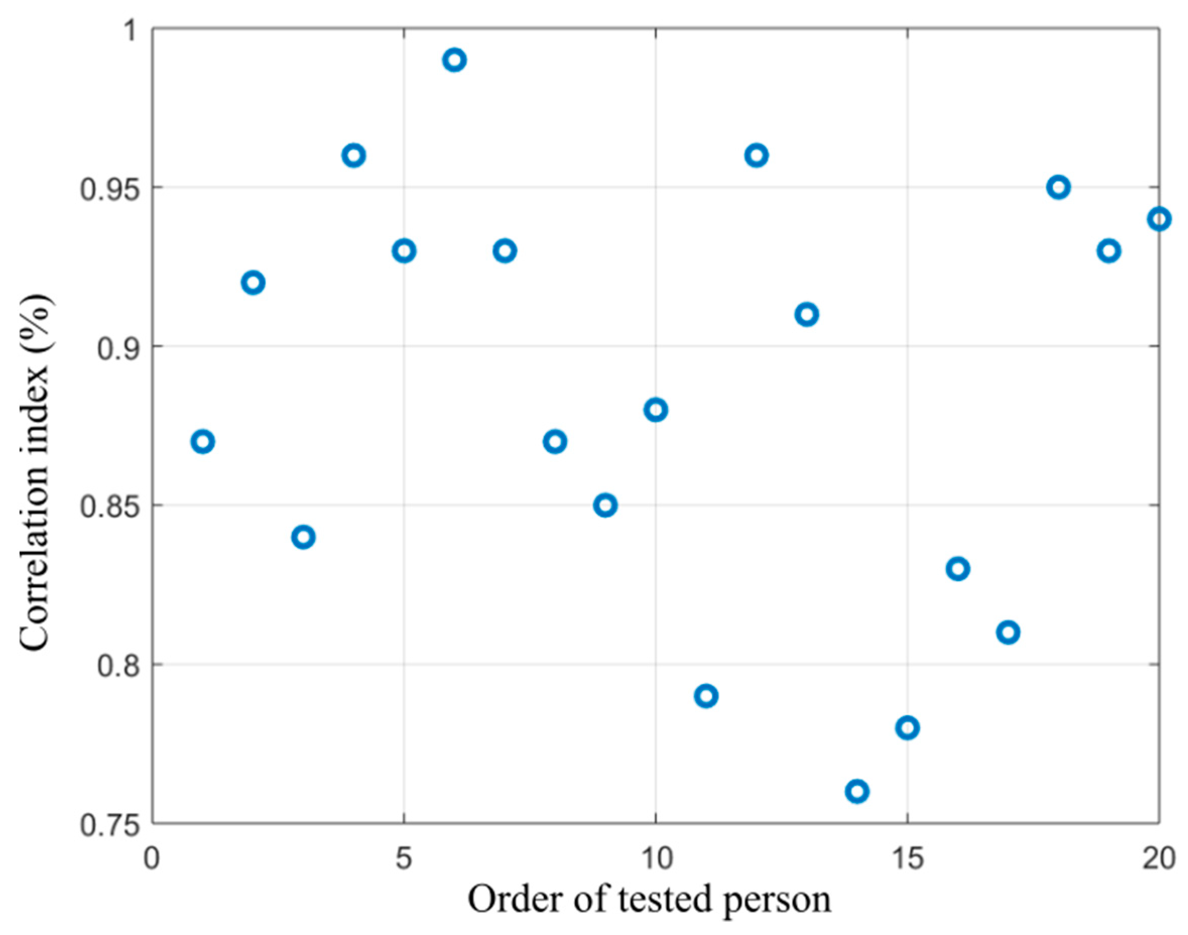
Figure 16.
Distribution of correlation index showing dependency between the alcohol content measured from breath and area size of the coldest area in the nose calculated from the proposed segmentation model.
Figure 16.
Distribution of correlation index showing dependency between the alcohol content measured from breath and area size of the coldest area in the nose calculated from the proposed segmentation model.
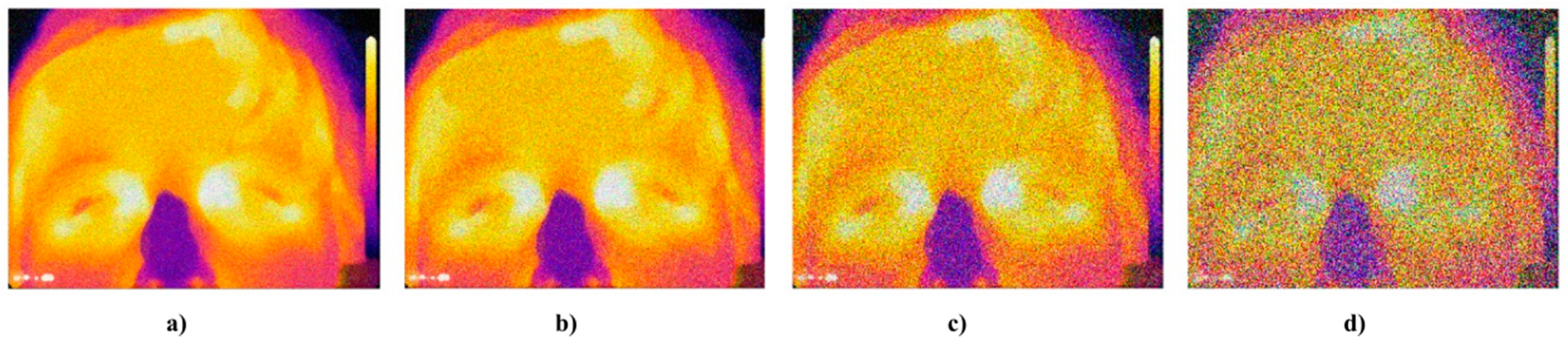
Figure 17.
Example of IR facial images corrupted by the Gaussian noise: (a) ), (b) ), (c) ), and (d) ).
Figure 17.
Example of IR facial images corrupted by the Gaussian noise: (a) ), (b) ), (c) ), and (d) ).
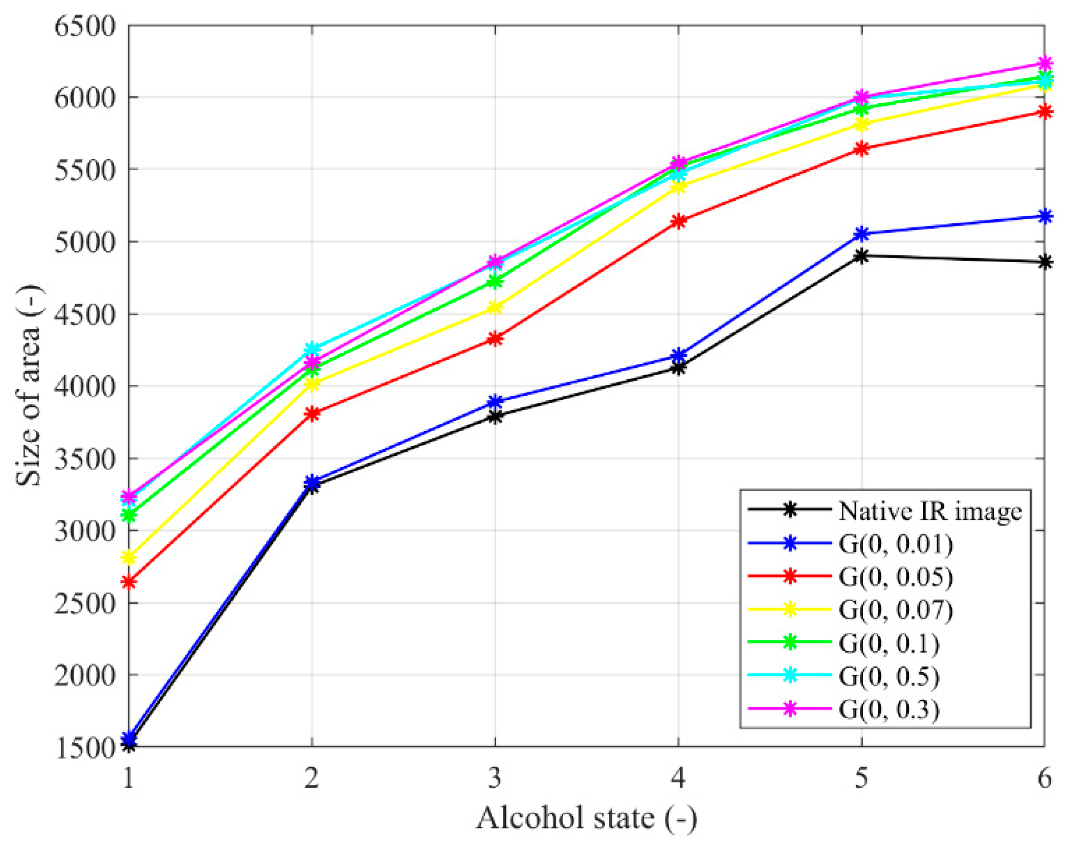
Figure 18.
Trend characteristic for Gaussian noise G(μ,σ2) with different settings μ = 0, σ2 = {0.01, 0.05, 0.07, 0.1, 0.3, 0.5}.
Figure 18.
Trend characteristic for Gaussian noise G(μ,σ2) with different settings μ = 0, σ2 = {0.01, 0.05, 0.07, 0.1, 0.3, 0.5}.
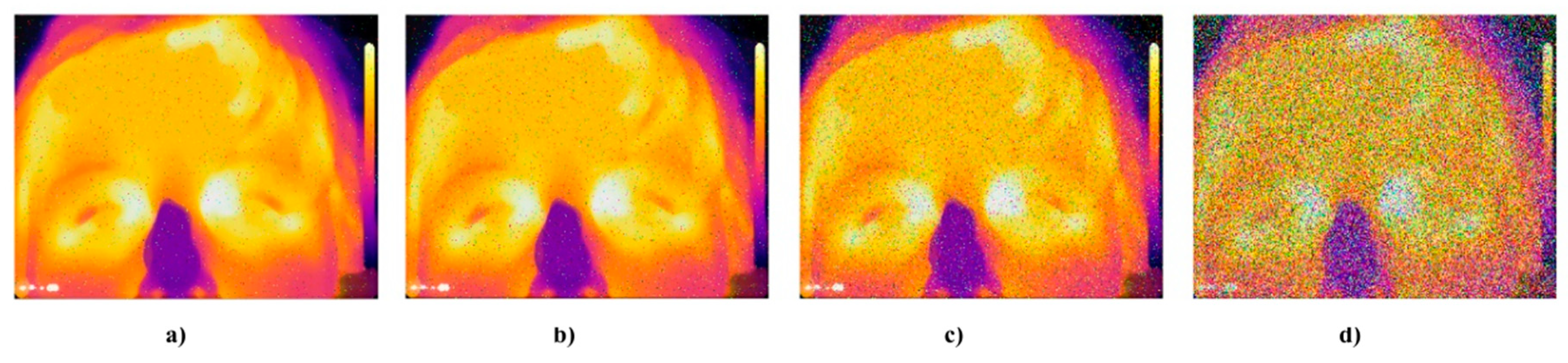
Figure 19.
Example of IR facial images corrupted by the Salt and Pepper: (a) SaP(0.01), (b) SaP(0.05), (c) SaP(0.07), and (d) SaP(0.5).
Figure 19.
Example of IR facial images corrupted by the Salt and Pepper: (a) SaP(0.01), (b) SaP(0.05), (c) SaP(0.07), and (d) SaP(0.5).
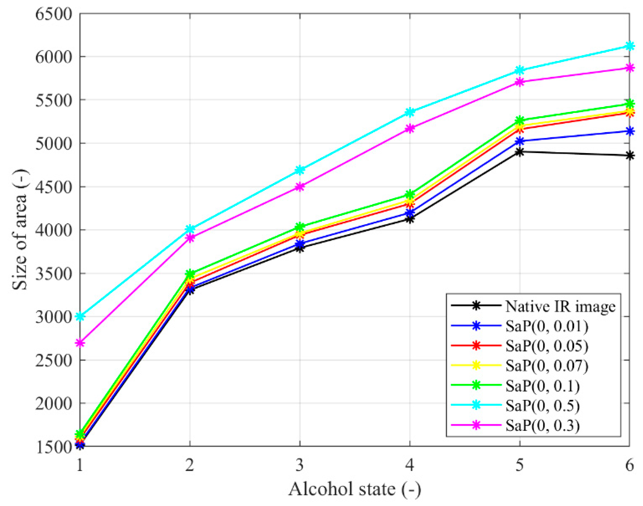
Figure 20.
Trend characteristic for the salt and pepper noise SaP(d) with different density settings: d = {0.01, 0.05, 0.07, 0.1, 0.3, 0.5}.
Figure 20.
Trend characteristic for the salt and pepper noise SaP(d) with different density settings: d = {0.01, 0.05, 0.07, 0.1, 0.3, 0.5}.
Figure 21.
Example of IR facial images corrupted by the salt and pepper: (a) μ = 0, σ2 = 0.01, (b) μ = 0, σ2 = 0.05, (c) μ = 0, σ2 = 0.3, and (d) μ = 0, σ2 = 0.5.
Figure 21.
Example of IR facial images corrupted by the salt and pepper: (a) μ = 0, σ2 = 0.01, (b) μ = 0, σ2 = 0.05, (c) μ = 0, σ2 = 0.3, and (d) μ = 0, σ2 = 0.5.
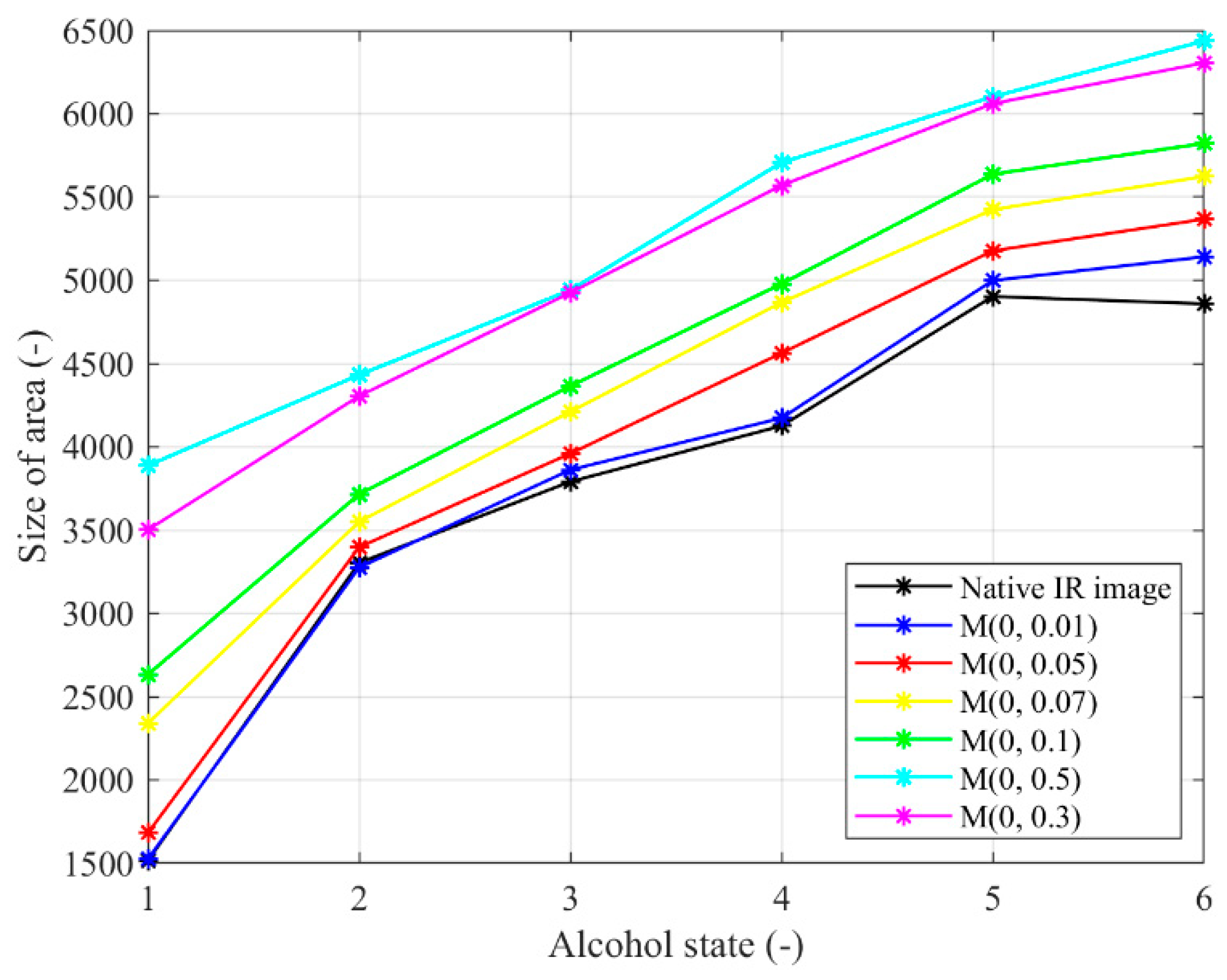
Figure 22.
Trend characteristic for the Multiplicative noise M(μ,σ2) with different settings: μ = 0,σ2 = {0.01, 0.05, 0.07, 0.1, 0.3, 0.5}.
Figure 22.
Trend characteristic for the Multiplicative noise M(μ,σ2) with different settings: μ = 0,σ2 = {0.01, 0.05, 0.07, 0.1, 0.3, 0.5}.
Table 1.
Classification of the acute alcohol intoxication.
Table 1.
Classification of the acute alcohol intoxication.
| Level of Intoxication | Level of Alcohol in Blood | Features |
|---|
| 1. Stage | Euphoria | <1% | Excitation, worsening of concentration |
| 2. Stage | Hypnotic | 1–2% | Disturbance of balance and movement coordination |
| 3. Stage | Narcotic | 2–3% | Disturbance of consciousness |
| 4. Stage | Asphyxia | >3% | Deep coma, hypothermia |
Table 2.
Extract of physiological parameters whilst alcohol intoxication measurement.
Table 2.
Extract of physiological parameters whilst alcohol intoxication measurement.
| Sex | Age | Height [m] | Weigh [kg] | Medicaments | Alcohol Breath [%] | Heart Rate [bpm] |
|---|
| w | 25 | 1.7500 | 62 | contraception | [0, 0.1700, 0.4300, 0.6700, 0.9100, 0.9200] | [82, 88, 81, 76, 75, 73] |
| m | 23 | 1.7800 | 70 | XYZAL | [0, 0.1200, 0.2900, 04900, 0.6800, 0.8700] | [70, 70, 67, 69, 60, 59] |
| m | 23 | 1.7900 | 85 | none | [0, 0.0900, 0.2400, 0.4000, 0.5600, 0.6500] | [86, 83, 83, 81, 85, 80] |
| m | 23 | 1.8200 | 78 | none | [0, 0.1700, 02900, 0.4600, 0.6300, 0.7200] | [58, 52, 53, 50, 51, 49] |
| m | 31 | 1.7700 | 65 | none | [0, 0.2300, 0.5400, 0.7400, 0.9400, 0.9500] | [93, 84, 78, 75, 73, 70] |
| w | 47 | 1.7200 | 100 | none | [0, 0.1600, 0.2600, 04200, 0.5500, 0.5900] | [93, 87, 86, 82, 79, 77] |
| w | 67 | 1.6700 | 95 | LORISTA | [0, 0.2100, 0.4100, 0.6400, 0.8500, 0.9300] | [80, 75, 68, 63, 63, 61] |
| m | 23 | 1.8200 | 90 | none | [0, 0.0100, 0.1600, 0.3900, 0.5200, 0.6900] | [66, 63, 70, 71, 73, 77] |
| m | 23 | 1.8600 | 87 | none | [0, 0.1700, 0.3200, 0.4900, 0.5800, 0.7100] | [50, 60, 56, 61, 63, 66] |
| m | 25 | 1.8800 | 92 | none | [0, 0.1900, 0.3200, 0.4500, 0.5900, 0.7200] | [50, 61, 56, 63, 63, 69] |
Table 3.
Dissimilarity measurement based on the Mean Squared Error (MSE).
Table 3.
Dissimilarity measurement based on the Mean Squared Error (MSE).
| Alcohol State | Nose | Forehead | Cheeks | Mouth |
|---|
| Sober state—100 mL of alcohol | 35.12 | 36.19 | 5.41 | 2.36 |
| Sober state—200 mL of alcohol | 44.12 | 49.58 | 6.69 | 5.78 |
Table 4.
Dissimilarity measurement based on the simple average differences.
Table 4.
Dissimilarity measurement based on the simple average differences.
| Alcohol State | Nose [%] | Forehead [%] | Cheeks [%] | Mouth [%] |
|---|
| Sober state—100 mL of alcohol | 19.56 | 22.11 | 3.95 | 1.15 |
| Sober state—200 mL of alcohol | 28.15 | 35.87 | 11.15 | 9.42 |
Table 5.
The average and best values for the objective function for three tested persons within the gradual alcohol intoxication. Testing for the image resolution: 640 × 480 px.
Table 5.
The average and best values for the objective function for three tested persons within the gradual alcohol intoxication. Testing for the image resolution: 640 × 480 px.
| Alcohol Content | Area of Interest | | | | | | |
|---|
| Person 1 | Person 2 | Person 3 |
|---|
| Sober state | Nose | 1.45 | 1.82 | 0.27 | 0.43 | 0.24 | 0.24 |
| Forehead | 3.49 | 8.74 | 0.52 | 1.22 | 0.10 | 0.36 |
| 40 mL | Nose | 1.54 | 1.55 | 0.32 | 0.84 | 0.27 | 0.58 |
| Forehead | 2.98 | 7.67 | 0.45 | 0.56 | 0.27 | 0.33 |
| 80 mL | Nose | 1.15 | 1.54 | 0.34 | 0.82 | 0.26 | 0.96 |
| Forehead | 2.45 | 8.00 | 0.48 | 1.12 | 0.43 | 1.66 |
| 120 mL | Nose | 1.47 | 5.20 | 0.29 | 0.62 | 0.29 | 0.38 |
| Forehead | 3.33 | 7.66 | 0.57 | 1.51 | 0.66 | 0.69 |
| 160 mL | Nose | 0.88 | 1.90 | 0.29 | 0.39 | 0.27 | 0.36 |
| Forehead | 2.92 | 10.14 | 0.53 | 1.03 | 0.55 | 1.27 |
Table 6.
The average and best values for the objective function for three tested persons within the gradual alcohol intoxication. Testing for the image resolution: 500 × 500 px.
Table 6.
The average and best values for the objective function for three tested persons within the gradual alcohol intoxication. Testing for the image resolution: 500 × 500 px.
| Alcohol Content | Area of Interest | | | | | | |
|---|
| Person 1 | Person 2 | Person 3 |
|---|
| Sober state | Nose | 1.62 | 1.87 | 0.38 | 0.42 | 0.28 | 0.25 |
| Forehead | 3.55 | 9.12 | 0.74 | 1.25 | 0.17 | 0.38 |
| 40 mL | Nose | 1.67 | 1.69 | 0.39 | 0.84 | 0.28 | 0.63 |
| Forehead | 3.12 | 7.87 | 0.84 | 0.92 | 0.32 | 0.41 |
| 80 mL | Nose | 1.17 | 1.64 | 0.41 | 0.64 | 0.32 | 1.14 |
| Forehead | 2.55 | 8.57 | 0.52 | 1.18 | 0.47 | 1.84 |
| 120 mL | Nose | 1.69 | 5.28 | 0.36 | 0.69 | 0.51 | 0.78 |
| Forehead | 3.87 | 7.69 | 0.61 | 1.67 | 0.69 | 0.84 |
| 160 mL | Nose | 1.14 | 1.96 | 0.35 | 0.85 | 0.32 | 0.42 |
| Forehead | 2.96 | 10.23 | 0.62 | 1.52 | 0.58 | 1.54 |
Table 7.
The average and best values for the objective function for three tested persons within the gradual alcohol intoxication. Testing for the image resolution: 300 × 300 px.
Table 7.
The average and best values for the objective function for three tested persons within the gradual alcohol intoxication. Testing for the image resolution: 300 × 300 px.
| Alcohol Content | Area of Interest | | | | | | |
|---|
| Person 1 | Person 2 | Person 3 |
|---|
| Sober state | Nose | 1.91 | 1.92 | 0.42 | 0.42 | 0.33 | 0.52 |
| Forehead | 3.85 | 9.55 | 0.86 | 1.44 | 0.45 | 0.45 |
| 40 mL | Nose | 1.59 | 1.67 | 0.41 | 0.92 | 0.32 | 0.71 |
| Forehead | 3.51 | 8.01 | 0.92 | 1.62 | 0.45 | 0.45 |
| 80 mL | Nose | 1.95 | 1.95 | 0.55 | 0.73 | 0.66 | 1.52 |
| Forehead | 2.62 | 8.68 | 0.56 | 1.62 | 0.55 | 1.87 |
| 120 mL | Nose | 1.74 | 5.36 | 0.45 | 0.76 | 0.58 | 0.65 |
| Forehead | 3.92 | 7.74 | 0.66 | 1.84 | 0.74 | 0.89 |
| 160 mL | Nose | 1.38 | 2.52 | 0.81 | 0.89 | 0.45 | 0.52 |
| Forehead | 3.15 | 10.44 | 0.71 | 1.68 | 0.99 | 1.66 |
Table 8.
The average and best values for the objective function for three tested persons within the gradual alcohol intoxication. Testing for the image resolution: 50 × 50 px.
Table 8.
The average and best values for the objective function for three tested persons within the gradual alcohol intoxication. Testing for the image resolution: 50 × 50 px.
| Alcohol Content | Area of Interest | | | | | | |
|---|
| Person 1 | Person 2 | Person 3 |
|---|
| Sober state | Nose | 2.45 | 2.54 | 1.84 | 1.22 | 1.12 | 1.42 |
| Forehead | 4.55 | 10.84 | 1.65 | 1.49 | 1.35 | 1.92 |
| 40 mL | Nose | 1.95 | 2.45 | 1.42 | 1.57 | 1.12 | 1.74 |
| Forehead | 3.84 | 8.63 | 1.38 | 1.63 | 1.65 | 1.95 |
| 80 mL | Nose | 2.21 | 2.45 | 1.69 | 1.91 | 1.31 | 1.69 |
| Forehead | 2.93 | 8.99 | 1.31 | 1.87 | 1.43 | 1.92 |
| 120 mL | Nose | 2.62 | 6.41 | 1.41 | 1.85 | 1.31 | 1.45 |
| Forehead | 4.81 | 7.84 | 1.56 | 2.32 | 1.36 | 1.89 |
| 160 mL | Nose | 1.83 | 2.76 | 1.21 | 1.84 | 1.12 | 1.52 |
| Forehead | 3.94 | 11.13 | 1.62 | 2.37 | 1.63 | 2.52 |
Table 9.
Time complexity for eight segmentation classes, SN = 100 and It = 100, p = 20% and.
Table 9.
Time complexity for eight segmentation classes, SN = 100 and It = 100, p = 20% and.
| Alcohol Content | Area of Interest | Time Complexity [s] |
|---|
| Person 1 | Person 2 | Person 3 |
|---|
| Sober State | Nose | 21.97 | 21.28 | 17.97 |
| Forehead | 33.27 | 22.67 | 20.52 |
| 40 mL | Nose | 23.66 | 19.41 | 17.02 |
| Forehead | 35.48 | 18.03 | 20.97 |
| 80 mL | Nose | 25.83 | 17.69 | 18.28 |
| Forehead | 33.67 | 19.25 | 20.57 |
| 120 mL | Nose | 23.01 | 18.89 | 19.57 |
| Forehead | 35.89 | 20.78 | 19.41 |
| 160 mL | Nose | 23.09 | 17.99 | 18.86 |
| Forehead | 33.43 | 19.52 | 20.70 |
| 200 mL | Nose | 25.87 | 17.33 | 18.75 |
| Forehead | 31.87 | 18.37 | 19.62 |
Table 10.
Time complexity for eight segmentation classes, SN = 70 and It = 90, p = 20%, and.
Table 10.
Time complexity for eight segmentation classes, SN = 70 and It = 90, p = 20%, and.
| Alcohol Content | Area of Interest | Time Complexity [s] |
|---|
| Person 1 | Person 2 | Person 3 |
|---|
| Sober State | Nose | 31.07 | 15.28 | 15.14 |
| Forehead | 25.07 | 16.32 | 16.75 |
| 40 mL | Nose | 16.96 | 15.15 | 15.97 |
| Forehead | 26.14 | 17.20 | 15.41 |
| 80 mL | Nose | 17.65 | 15.33 | 15.64 |
| Forehead | 28.70 | 14.94 | 15.42 |
| 120 mL | Nose | 18.72 | 14.86 | 14.98 |
| Forehead | 30.72 | 15.42 | 16.70 |
| 160 mL | Nose | 18.78 | 15.12 | 14.02 |
| Forehead | 24.25 | 16.29 | 15.72 |
| 200 mL | Nose | 16.20 | 15.72 | 14.83 |
| Forehead | 25.07 | 15.33 | 17.16 |
Table 11.
Time complexity for eight segmentation classes, SN = 120 and It = 60, p = 20%, and.
Table 11.
Time complexity for eight segmentation classes, SN = 120 and It = 60, p = 20%, and.
| Alcohol Content | Area of Interest | Time Complexity [s] |
|---|
| Person 1 | Person 2 | Person 3 |
|---|
| Sober State | Nose | 18.42 | 14.97 | 14.98 |
| Forehead | 25.19 | 16.37 | 15.75 |
| 40 mL | Nose | 18.89 | 14.88 | 14.58 |
| Forehead | 26.93 | 15.24 | 15.43 |
| 80 mL | Nose | 16.92 | 15.19 | 14.87 |
| Forehead | 26.05 | 16.09 | 14.76 |
| 120 mL | Nose | 17.49 | 14.47 | 14.96 |
| Forehead | 25.83 | 16.26 | 14.97 |
| 160 mL | Nose | 15.88 | 13.10 | 15.14 |
| Forehead | 28.46 | 14.59 | 15.04 |
| 200 mL | Nose | 17.11 | 14.06 | 14.21 |
| Forehead | 24.48 | 15.49 | 16.78 |
Table 12.
Quantitative comparison for the native IR images (640 × 480 px).
Table 12.
Quantitative comparison for the native IR images (640 × 480 px).
| | Proposed | Otsu | K-Means | FCM | RG |
|---|
| Corr | 0.94 | 0.91 | 0.88 | 0.93 | 0.74 |
| RI | 0.91 | 0.88 | 0.81 | 0.92 | 0.71 |
| VI | 3.11 | 3.21 | 4.15 | 4.11 | 5.01 |
| MSE | 28.45 | 35.87 | 36.12 | 29.98 | 36.88 |
Table 13.
Quantitative comparison for the Gaussian noise: , (640 × 480 px).
Table 13.
Quantitative comparison for the Gaussian noise: , (640 × 480 px).
| | Proposed | Otsu | K-Means | FCM | RG |
|---|
| Corr | 0.91 | 0.88 | 0.84 | 0.82 | 0.69 |
| RI | 0.91 | 0.82 | 0.75 | 0.87 | 0.66 |
| VI | 2.98 | 3.27 | 5.11 | 4.52 | 5.44 |
| MSE | 31.52 | 34.57 | 33.18 | 31.99 | 38.74 |
Table 14.
Quantitative comparison for the Gaussian noise: , (640 × 480 px).
Table 14.
Quantitative comparison for the Gaussian noise: , (640 × 480 px).
| | Proposed | Otsu | K-Means | FCM | RG |
|---|
| Corr | 0.88 | 0.75 | 0.81 | 0.69 | 0.48 |
| RI | 0.74 | 0.76 | 0.45 | 0.66 | 0.43 |
| VI | 3.87 | 4.12 | 5.56 | 4.75 | 7.57 |
| MSE | 33.87 | 36.88 | 34.12 | 35.41 | 39.45 |
Table 15.
Quantitative comparison for the Salt and Pepper noise:, (640 × 480 px).
Table 15.
Quantitative comparison for the Salt and Pepper noise:, (640 × 480 px).
| | Proposed | Otsu | K-Means | FCM | RG |
|---|
| Corr | 0.93 | 0.79 | 0.86 | 0.88 | 0.69 |
| RI | 0.91 | 0.93 | 0.88 | 0.91 | 0.66 |
| VI | 3.54 | 4.18 | 5.48 | 4.12 | 6.55 |
| MSE | 28.45 | 30.12 | 31.15 | 34.47 | 36.84 |
Table 16.
Quantitative comparison for the Salt and Pepper noise: , (640 × 480 px).
Table 16.
Quantitative comparison for the Salt and Pepper noise: , (640 × 480 px).
| | Proposed | Otsu | K-Means | FCM | RG |
|---|
| Corr | 0.79 | 0.65 | 0.66 | 0.71 | 0.38 |
| RI | 0.84 | 0.83 | 0.75 | 0.74 | 0.41 |
| VI | 5.12 | 5.99 | 7.84 | 6.12 | 6.77 |
| MSE | 33.54 | 31.85 | 33.45 | 33.32 | 39.85 |
Table 17.
Quantitative comparison for the Multiplicative noise: (640 × 480 px).
Table 17.
Quantitative comparison for the Multiplicative noise: (640 × 480 px).
| | Proposed | Otsu | K-Means | FCM | RG |
|---|
| Corr | 0.88 | 0.78 | 0.69 | 0.76 | 0.64 |
| RI | 0.91 | 0.82 | 0.83 | 0.79 | 0.68 |
| VI | 2.99 | 3.21 | 5.34 | 4.63 | 7.11 |
| MSE | 32.84 | 32.65 | 34.56 | 36.93 | 41.12 |
Table 18.
Quantitative comparison for the Multiplicative noise: (640 × 480 px).
Table 18.
Quantitative comparison for the Multiplicative noise: (640 × 480 px).
| | Proposed | Otsu | K-Means | FCM | RG |
|---|
| Corr | 0.74 | 0.68 | 0.61 | 0.59 | 0.48 |
| RI | 0.75 | 0.74 | 0.81 | 0.54 | 0.48 |
| VI | 3.16 | 3.93 | 5.91 | 5.17 | 8.15 |
| MSE | 33.54 | 32.89 | 36.45 | 39.62 | 44.19 |
Table 19.
Parameters settings for the modified Artificial Bee Colony (ABC) algorithm.
Table 19.
Parameters settings for the modified Artificial Bee Colony (ABC) algorithm.
| Parameter | Value |
|---|
| Number of food sources (SN) | |
| Number of iterations (It) | |
| selection limit | |
| Lower limitation () and upper limitation () | |
Table 20.
Parameters settings for the ABC algorithm.
Table 20.
Parameters settings for the ABC algorithm.
| Parameter | Value |
|---|
| Number of food sources (SN) | |
| Number of iterations (It) | |
| selection limit | |
| Lower limitation () and upper limitation () | |
Table 21.
Parameters settings for the Particle Swarm Optimization (PSO) algorithm.
Table 21.
Parameters settings for the Particle Swarm Optimization (PSO) algorithm.
| Parameter | Value |
|---|
| Swarm size | |
| Number of iterations (It) | |
| Cognitive, social and neighborhood acceleration | |
| Lower limitation () and upper limitation () | |
| Error goal | 1 × 10⁻⁶ |
| Maximal trial limit | 450 |
| Value of velocity weight at the end of the PSO iterations | 0.3 |
| Value of velocity weight at the beginning of the PSO | 0.97 |
| The fraction of the maximum iterations, for which W is linear evolved | 0.6 |
| Value of global minimum | 0 |
Table 22.
Parameters settings for the GA.
Table 22.
Parameters settings for the GA.
| Parameter | Value |
|---|
| Population size | |
| Number of iterations (It) | |
| Crossover probability | |
| Mutation probability | |
| Number of bits for each variable | 7 |
| Eta () | 1 |
| Lower limitation () and upper limitation () | |
Table 23.
Quantitative comparison for modified ABC, ABC, GA and Particle Swarm Optimization (PSO) based on the Peak Signal-to-Noise Ratio (PSNR) [dB].
Table 23.
Quantitative comparison for modified ABC, ABC, GA and Particle Swarm Optimization (PSO) based on the Peak Signal-to-Noise Ratio (PSNR) [dB].
| Testing IR Image [px] | n | PSNR [dB] |
|---|
| Modified ABC | ABC | GA | PSO |
|---|
| 640 × 480 | 1 | 27.11 | 26.54 | 26.99 | 29.98 |
| 2 | 27.03 | 26.45 | 26.98 | 26.92 |
| 3 | 26.78 | 25.92 | 26.74 | 27.78 |
| 4 | 26.77 | 26.54 | 25.84 | 26.71 |
| 5 | 27.13 | 27.11 | 26.87 | 26.98 |
| 500 × 500 | 1 | 25.12 | 25.01 | 24.33 | 24.98 |
| 2 | 26.12 | 25.87 | 25.44 | 25.51 |
| 3 | 25.45 | 25.32 | 25.87 | 24.65 |
| 4 | 26.17 | 25.93 | 25.45 | 26.01 |
| 5 | 24.65 | 24.87 | 25.11 | 24.84 |
| 300 × 300 | 1 | 24.45 | 23.44 | 23.87 | 24.15 |
| 2 | 23.98 | 23.65 | 24.11 | 24.05 |
| 3 | 24.54 | 24.21 | 23.59 | 23.93 |
| 4 | 23.84 | 23.45 | 23.11 | 23.81 |
| 5 | 22.84 | 23.13 | 24.54 | 23.41 |
| 50 × 50 | 1 | 21.45 | 21.21 | 21.35 | 20.48 |
| 2 | 21.65 | 21.36 | 20.48 | 20.16 |
| 3 | 20.84 | 20.65 | 20.94 | 21.13 |
| 4 | 21.32 | 20.45 | 20.84 | 20.44 |
| 5 | 21.55 | 20.98 | 20.74 | 21.43 |
Table 24.
Quantitative comparison for modified ABC, ABC, GA, and PSO based on the SSIM.
Table 24.
Quantitative comparison for modified ABC, ABC, GA, and PSO based on the SSIM.
| Testing IR Image [px] | n | SSIM |
|---|
| Modified ABC | ABC | GA | PSO |
|---|
| 640 × 480 | 1 | 0.94 | 0.87 | 0.72 | 0.91 |
| 2 | 0.98 | 0.91 | 0.94 | 0.79 |
| 3 | 0.89 | 0.91 | 0.78 | 0.88 |
| 4 | 0.93 | 0.91 | 0.87 | 0.88 |
| 5 | 0.96 | 0.89 | 0.73 | 0.79 |
| 500 × 500 | 1 | 0.77 | 0.81 | 0.74 | 0.75 |
| 2 | 0.90 | 0.73 | 0.79 | 0.89 |
| 3 | 0.59 | 0.93 | 0.69 | 0.78 |
| 4 | 0.79 | 0.71 | 0.73 | 0.74 |
| 5 | 0.82 | 0.83 | 0.76 | 0.77 |
| 300 × 300 | 1 | 0.65 | 0.67 | 0.45 | 0.59 |
| 2 | 0.64 | 0.61 | 0.52 | 0.59 |
| 3 | 0.74 | 0.71 | 0.68 | 0.69 |
| 4 | 0.82 | 0.81 | 0.74 | 0.58 |
| 5 | 0.79 | 0.81 | 0.78 | 0.80 |
| 50 × 50 | 1 | 0.66 | 0.61 | 0.62 | 0.65 |
| 2 | 0.69 | 0.45 | 0.49 | 0.53 |
| 3 | 0.74 | 0.75 | 0.73 | 0.65 |
| 4 | 0.78 | 0.65 | 0.67 | 0.69 |
| 5 | 0.74 | 0.76 | 0.74 | 0.81 |
Table 25.
Quantitative comparison for modified ABC, ABC, GA, and PSO based on the FSIM.
Table 25.
Quantitative comparison for modified ABC, ABC, GA, and PSO based on the FSIM.
| Testing IR Image [px] | n | FSIM |
|---|
| Modified ABC | ABC | GA | PSO |
|---|
| 640 × 480 | 1 | 0.88 | 0.84 | 0.87 | 0.83 |
| 2 | 0.95 | 0.77 | 0.81 | 0.93 |
| 3 | 0.91 | 0.88 | 0.89 | 0.93 |
| 4 | 0.79 | 0.77 | 0.68 | 0.78 |
| 5 | 0.87 | 0.86 | 0.86 | 0.84 |
| 500 × 500 | 1 | 0.69 | 0.72 | 0.73 | 0.75 |
| 2 | 0.72 | 0.71 | 0.65 | 0.71 |
| 3 | 0.83 | 0.81 | 0.79 | 0.68 |
| 4 | 0.81 | 0.74 | 0.79 | 0.80 |
| 5 | 0.78 | 0.81 | 0.78 | 0.81 |
| 300 × 300 | 1 | 0.65 | 0.69 | 0.64 | 0.64 |
| 2 | 0.72 | 0.71 | 0.59 | 0.63 |
| 3 | 0.65 | 0.69 | 0.61 | 0.59 |
| 4 | 0.78 | 0.71 | 0.73 | 0.74 |
| 5 | 0.77 | 0.73 | 0.74 | 0.68 |
| 50 × 50 | 1 | 0.59 | 0.57 | 0.45 | 0.53 |
| 2 | 0.54 | 0.51 | 0.52 | 0.61 |
| 3 | 0.61 | 0.54 | 0.59 | 0.60 |
| 4 | 0.68 | 0.55 | 0.58 | 0.59 |
| 5 | 0.71 | 0.68 | 0.56 | 0.70 |

 ,
, 


