Abstract
The movement of the gantry crane is controlled by an symmetry underactuated system, and has poor robustness in precise positioning. A new active control method based on the machine vision positioning is proposed in this paper, and the trajectories are planned after the detection of starting and ending points. A new type of energy storage function is given in this paper, and a coupling control law is derived to minimize the load swing in the process of precise positioning. The equilibrium point of the closed-loop system is checked though Lyapunov and LaSalle’s theorems, and the calculation results are verified through experimental investigations. The results show that the equilibrium points are asymptotically stable, and the proposed control method is of better robustness. The findings provide a new kind of control method with higher efficiency, and can help with the precise control of gantry cranes.
1. Introduction
Gantry cranes have the advantages of high payload capacity, good operational flexibility, and less energy consumption, and are widely used in loading and transportation processes at material yards and ports. The payload is led to the reserved position by the control system, and the unexpected payload oscillation is designed to be minimized. The swing freedom of the payload lacks the driver to control. Therefore, the control system of the gantry crane is symmetry underactuated, and is of poor robustness because the independent control inputs are fewer than the degrees of freedom (DOF). During the past several decades, the control system has attracted research interests from many researchers. Fang et al. [1] proposed a control scheme based on motion planning and adaptive crane underactuated system, which can still achieve good control performance under unknown system parameters. Pezeshki et al. [2] proposed a feedback linearized modelless adaptive controller and a fuzzy approximation adaptive sliding membrane controller to control the underactuated crane system. Sun et al. designed a crane underactuated control strategy based on the energy optimal solution [3] and quasi-proportional integral derivative (PID) [4], considering the hook and payload double swing problem. Lu et al. [5] designed a dual crane cooperative operation controller, and proved the stability of the system to equilibrium point by using Lyapunov techniques and LaSalle’s invariance theorem. Most of the studies focused on the passive target control, and the target positions need to be input several times in consecutive works during lifting and translation. Multiple manual inputs lead to accumulative errors, and the accuracy and efficiency are decreased. Therefore, a control system with high accuracy and robustness is needed.
The active control system takes the working conditions into consideration, and can reduce the payload oscillation in the working process. Visual systems are widely applied in active control systems, and the accumulative errors brought by the multiple position inputs can be minimized. For the studies of vision-based active control systems, Yasir et al. [6] proposed a combination of visible light and smartphone acceleration sensors. Hossen et al. [7] used a combination of computer vision sensors and visible light communication with light-emitting diodes (LED). Truc [8] designed a navigation method for ground fuzzy line tracking and quick response (QR) code recognition. The above methods have achieved good results in the application of visual positioning and detection, and the control precision is proven to be improved compared with the passive control systems. The control strategies of the vision-based systems are derived from the motions of the objectives, and are closely related with the dynamic characteristics of the system. Recent applications of the control system on the gantry crane mostly focus on the two-dimensional (2D) motions, and only the oscillation motions in the trolley plane are taken into consideration. However, the payload moves in a three-dimensional (3D) space when the trolley and the gantry move simultaneously, and the impact of gantry motion on the oscillation cannot be ignored, as shown in Figure 1.
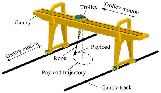
Figure 1.
Motions of the 3D gantry crane and payload.
There are two general kinematic structures for 2D gantry cranes. Firstly, the gantry is transferred in the X direction, at which time the trolley does not transfer; secondly, the trolley is transferred in the Y direction, but the gantry is fixed. The general kinematic structure of a 3D gantry crane refers to the movement of the gantry in the X direction while the trolley is transferring in the Y direction. The oscillation of the payload is affected by the coupling motions of the gantry and the trolley; therefore, the motion of the payload shows nonlinear changes. Moustafa et al. [9] used the Lagrange method to establish a dynamic model of a 3D crane. A linear feedback control system is proposed to realize the anti-swing motion control of the crane under various motion states. Fang et al. [10] designed several nonlinear feedback controllers for the underactuated gantry crane with constant rope length, which realized the “micro-swing” control of the system. Tuan et al. [11] designed a second-order synovial controller for gantry cranes with uncertain system parameters. Wu et al. [12] designed a 3D crane partial feedback linearization controller. The new swing suppression unit and the positioning error signal are constructed to ensure effective suppression of the rapid transferring and swing of the payload. Zhang [13] designed an enhanced coupled nonlinear tracking control method for underactuated 3D crane systems. However, changes in system parameters such as the mass of the payload and the length of the rope were not taken into consideration in these studies, which is not consistent with the actual situations. Furthermore, the external load is not included in the models, and the swing angle exceeded the threshold when the system was faced with external disturbance.
As discussed above, the lack of precise control of an underactuated gantry crane system is the result of the inaccurate dynamic model and improper control method. Therefore, a precise model of the 3D payload motion with the vision-based active control method is quite essential. In this paper, a precise 3D dynamic model including the coupling effect of gantry and trolley motions is proposed, and a method of machine vision recognition using QR code artificial beacons is put forward. The QR code is applied to obtain the coordinates of the start and end positions of the payload transfer, and a nonlinear control law based on energy coupling is designed for the precise control of the payload. As the main contribution of this paper, the proposed method successfully merges the advantages of machine vision positioning and energy-based control law, achieving an improved control performance. They are presented as follows:
- (1)
- The newly designed machine visual positioning system improves the positioning accuracy and automation efficiency of the gantry crane.
- (2)
- The control law has a concise structure without requiring exact knowledge of system parameters, which is convenient for practical implementation. It is robust against external disturbances, which is validated by experimental results.
The contents are as follows. The overall design of control method is given in the Section 2, and the dynamic model is described in Section 3. The machine vision positioning system is introduced in Section 4, and the trajectory planning is designed in Section 5. The control law is designed and analyzed in Section 6. In Section 7, there are simulation and experimental investigations on a gantry crane test rig to verify the performance of the designed control system, and finally the conclusions are drawn.
2. Control Method Design
This section describes the implementation steps of the underactuated gantry crane control method based on machine vision positioning.
Step 1: The 3D dynamic model of the gantry crane was built using the Euler–Lagrange equation.
Step 2: The multi-state nonlinear coupled differential equation of the gantry crane is obtained by solving the dynamic equation. Obtaining a trolley, the payload swing angle is based on a function of time when the gantry is operating at a constant acceleration.
Step 3: Image acquisition of gantry crane working surface, image preprocessing, detection of payload transfer end point, and calculation of target displacement of trolley and gantry.
Step 4: The payload swing angle obtained in step 2 is based on the time function, and the trolley and gantry frame obtained in step 3 are displaced. The trajectory planning strategy of the trolley, the trajectory planning strategy of the gantry, and the planning strategy of the payload trajectory are designed.
Step 5: A new energy function is constructed. On the basis of the multi-state nonlinear coupled differential equation of the gantry crane obtained in step 2, the non-linear trolley based on energy coupling and the gantry operating control law are designed. The stability of the closed-loop control system is proven by the Lyapunov techniques and Lasalle’s invariance theorem.
Step 6: The target displacement of the trolley and the gantry frame obtained in step 3 and the control law obtained in step 5 are input into the trolley and the gantry controller, respectively. The controller controls the drive to drive the trolley and the gantry’s motion motor mechanical system with voltage signals. The encoder feeds the trolley, the gantry displacement, and the payload swing angle information to the controller in real time with the pulse signal. Under the action of the closed-loop control system, the trolley and the gantry run smoothly, and the payload swing angle is effectively suppressed within the safe range.
Step 7: End. The trolley and the gantry are accurately moved to the target position, and the payload residual swing angle is eliminated.
The overall schematic diagram of the underactuated gantry crane control method based on machine vision positioning is shown in Figure 2.

Figure 2.
Control method diagram.
3. Gantry Crane Dynamics Modeling
The schematic diagram of the gantry crane is shown in Figure 3. The gantry crane dynamics model is established using the Euler–Lagrange equation [14]:
where represents the state vector of the gantry crane system; represents the inertia matrix of the system; represents the centripetal-Coriolis force matrix of the system; represents the gravitational potential energy vector of the system; and represents the control vector of the system. The specific definition of the above parameters is as follows:
where represents the sum of the mass of the gantry and the trolley; indicates the mass of the trolley; represents the payload mass; indicates the length of the sling rope; represents the acceleration of gravity; and represent the payload swing angle generated by the X direction operation of the gantry and the Y direction operation of the trolley, respectively; and and stand for the resultant force applied to the gantry and trolley, respectively, which consists of the following two parts:
where and denote the actuating force of the gantry and the trolley, respectively; donates the mechanical friction between the gantry and the rail; and donates the friction between the trolley and the gantry. Inspired by the friction model presented in the work of [15] and after some experimental studies, we utilize the following model to describe the friction:
where , and are the friction-related parameters to be determined.
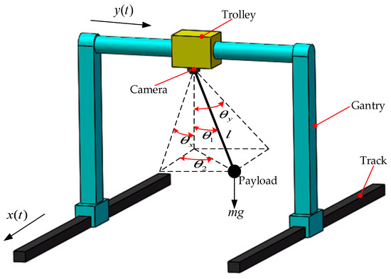
Figure 3.
Gantry crane dynamics model.
4. Machine Vision Positioning System
The QR code [16] is tiled on the working surface of the gantry crane at regular intervals (see Figure 4). We use the QR code as the target point to establish the positioning coordinate system. Firstly, the image of the collected gantry crane working surface is preprocessed, then the target is detected and positioned, and finally the machine vision positioning system is established.

Figure 4.
Machine vision positioning system.
4.1. Image Preprocessing
In order to improve the real-time performance of data analysis and processing, eliminate the influence of irrelevant information, and improve the detectability of effective information, it is necessary to preprocess the original image of the working plane of the gantry crane shot by the HD industrial camera. Preprocessing of the original image includes grayscale, binarization, and Canny edge detection.
The process of converting a color image into a grayscale image is called grayscale processing of the image. The RGB color image is a combination of three different color components: red (R), green (G), and blue (B). Each pixel in the grayscale image can be represented by a luminance value of 0 to 255. We use the weighted averaging algorithm of (9) to grayscale the color image:
Image binarization is used to set the gray value of the pixel on the image to 0 (black) or 255 (white). Converting 256 luminance level grayscale images to binarized images with appropriate threshold selection can still reflect the overall and local features of the image. The binarized image presents a black and white effect that highlights the contrast between the target image and the background. The image binarization formula is as follows:
where represents the threshold.
Canny edge detection is a multi-level edge detection algorithm. The Canny edge detection algorithm can be divided into the following five steps [17,18]: (1) use a Gaussian filter to smooth the image and filter out noise; (2) calculate the gradient strength and direction of each pixel in the image; (3) apply non-maximum suppression to eliminate spurious responses from edge detection; (4) apply dual threshold detection to determine true and potential edges; (5) finalize edge detection by suppressing isolated weak edges.
4.2. Target Detection and Positioning
The camera uses the principle of small hole imaging. The world coordinate system and the image pixel coordinate system can be converted by a linear camera model. The camera imaging principle is shown in Figure 5.
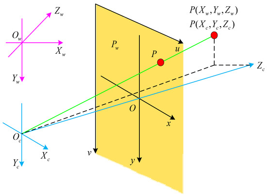
Figure 5.
Camera calibration principle.
The camera coordinate conversion relationship is as follows [19,20]:
where is the focal length, and represent the unit pixel size of the image in the X direction and the Y direction, respectively; represent the coordinates of the principal point of the pixel coordinate system; is a rotation matrix; is a translation vector; is a parameter matrix within the camera; is the parameter matrix outside the camera; and is a camera parameter matrix.
In order to determine the location of the pixel plane where the QR code (see Figure 6) target is located, we use the OpenCV [21,22] computer vision library. The findContours function is used to extract the boundary contours of a, b, and c of the QR code in the preprocessed picture. The 4 corner points of d (d − 1, d − 2, d − 3, d − 4) can then be inferred from the 12 corner points of a (a − 1, a − 2, a − 3, and a − 4), b (b − 1, b − 2, b − 3, and b − 4), and c (c − 1, c − 2, c − 3, and c − 4). We can determine the smallest rectangle surrounding the QR code based on the four corner points (a − 1, b − 2, c − 3, and d − 4), and the image coordinates of center point are shown as follows:

Figure 6.
QR code.
Image center pixel point coordinates and QR code target center point pixel coordinates based on the pixel coordinate system can be obtained. Substituting the coordinate system conversion Formula (11), the coordinates of the target point of the world coordinate system can be obtained by the Formula (13). In the world coordinate system, the payload projection point is the transition starting point, and the QR code center point is the transition end point. The target displacement and of the trolley and gantry can be obtained by (14).
5. Trajectory Planning
In order to achieve accurate and smooth control of the gantry crane, the trajectory of the gantry and trolley should meet a smooth S-shaped curve [23]. First, we introduce a three-stage acceleration trajectory to make the gantry run separately in the X direction. Its expression is as follows:
where , , and represent the acceleration, velocity, and target displacement of the gantry in the X direction, respectively; represents the maximum acceleration; and and indicate the acceleration/deceleration time and the uniform speed time, respectively. , , and can be obtained from the following equations [24]:
where , , and represent the preset acceleration, speed, and swing angle upper limit of the X direction running system of the gantry, respectively; represents an acceleration/deceleration cycle; and represents the natural frequency of the system and is related to the length of the sling.
The differential equation for the dynamic coupling relationship between the acceleration of the gantry and the swing angle of the payload can be obtained by the expansion of (1):
The actual gantry crane system meets , [25,26,27,28,29]. Therefore, Equation (22) can be expressed as a partial differential equation:
When the gantry is running at a constant acceleration , Equation (23) can be solved as follows, and the payload swing angle is obtained as a function of time :
where and represent the initial angle and angular velocity of the gantry in the X direction, and the actual conditions satisfy .
The trajectory planning of the gantry crane trolley in the Y direction can refer to the operation law of the gantry in the X direction, and will not be described here.
In order to improve the operating efficiency, the gantry and trolley often run simultaneously in practical applications. In the compound direction, acceleration , speed , displacement , swing angle , swing angle , plus/deceleration time , and uniform speed time are defined as follows:
6. Control Law Design and Stability Analysis
6.1. Control Law Design
The energy function shown below is constructed from the mechanical energy of the gantry crane:
where
We hope to enhance the dynamic coupling relationship between the displacement of the gantry ; the displacement of the trolley ; and the swing angle of the payload , . Therefore, a positive definite scalar function as shown below is constructed based on the energy function form:
where are positive control gains; is the positioning errors of the payload in the X direction; and is the positioning errors of the payload in the Y direction:
where represents the errors between the actual displacement of the gantry and the target displacement in the X direction, and represents the errors between the actual displacement of the trolley and the target displacement in the Y direction. They are defined as follows:
For to refer to time, substituting (1), we get the following:
On the basis of the form shown in , design the controller is shown below:
where are positive control gains.
6.2. Closed-Loop System Stability Analysis
Theorem 1.
Under the control law (38), the gantry and trolley running displacements converge to the target displacement, and the payload swing angle is suppressed and eliminated. Satisfy the following theorem:
Proof.
The positive definite scalar function of (30) is chosen as the Lyapunov candidate function. We substitute the control law (38) into (37) and get the following formula:
which shows that the gantry crane closed-loop control system is Lyapunov stable at the origin. In consequence, it is easily concluded that
and the closed-loop system state is bounded. Therefore,
To accomplish the proof, let be the largest invariant set in , where
Then, based on (40), the following is clear in :
Therefore, the following conclusions can be drawn:
where are pending constants. in the maximum variable set will then be demonstrated. Combining (1), (38), (44), and (46), we get the following:
Therefore, will vary at a constant speed as shown in Equation (46), assuming , which implies the following:
Obviously, this contradicts Equation (42), so the assumption is incorrect. Therefore,
Then, from Equations (37), (43), (44), (46), and (48), we get the following:
where are constants to be determined. In the maximum invariant set , the same analysis as above shows the following:
where are the constants to be determined. It will then be proven that in the largest constant set .
First, assume that , by combining (50) and (55), we can obtain the following equation set:
The condition in (22) is imported in (52), and we get the following:
Combining Equations (46), (52), (56), and (57), the following equation can be obtained:
The condition in (44) is imported in (54), and we get the following:
Solving the system of Equations (58) and (59) gives the following:
It can be further inferred that in the maximum invariant set ,
Obviously, Equation (61) contradicts Equation (57), so it is assumed that does not hold. Therefore, is satisfied in the maximum invariant set , thereby inferring the following:
Therefore, combining (50) and (58) shows
On the basis of the above analysis, it can be known that the maximum invariant set contains only the equilibrium point .
According to the LaSalle’s invariance theorem [30], the closed-loop system converges to equilibrium point with time under the control law (38). Therefore, the Theorem 1 is proved. □
7. Simulation Experiment and Result Analysis
7.1. Machine Vision Positioning Experimental Results and Analysis
The machine vision positioning experiment is carried out on the gantry crane test bench (See Figure 7). The HD industrial camera in our vision system is a Mercury series camera made by Daheng IMAVISION (see Figure 8), of which the frame rate is 120 fps, the pixel size is 5.6 um × 5.6 um, the focal length is 3.5 mm, and the exposure time is also adjustable. The camera is fixedly mounted under the center of the trolley. The camera plane is parallel to the ground. As the gantry is highly fixed, the camera moves with the trolley at a fixed height plane.

Figure 7.
Gantry crane test bench.

Figure 8.
MER-1220-32U3M/C.
We analyzed the image of the gantry crane working surface. Image preprocessing not only reduces the amount of data computation, but also helps extract useful information about the target and background. Then, we use the target recognition and localization algorithm to determine the target displacement of the trolley and the gantry.
The processing of the image of the working plane of the gantry crane is shown in Figure 9. The final recognition result based on machine vision positioning is shown in Figure 10. It can be seen that and .
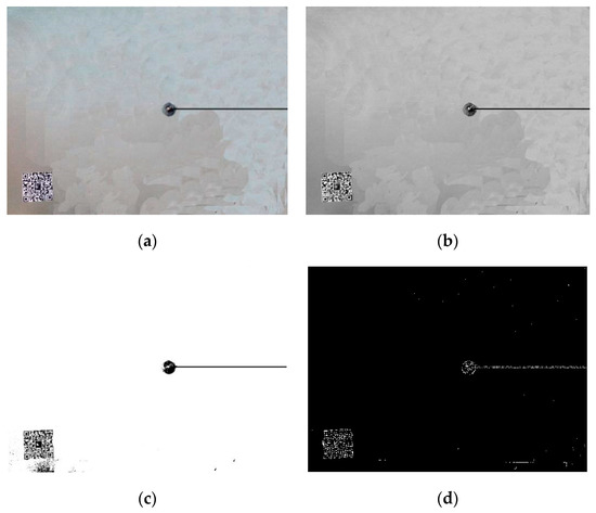
Figure 9.
Image preprocessing. (a) Original image; (b) grayscale image; (c) binary chart; (d) Canny edge detection.

Figure 10.
Identifying the positioning result.
7.2. Friction Simulation and Analysis
For this article, we employ the compensation method for the nonlinear friction. To this end, the friction model of (8) is utilized as a feedforward component to compensate for the track friction. After plenty of simulation test, the friction parameters in (8) are determined as , , , , , and .
On the basis of the simulation results shown in Figure 11, it is concluded that friction changes with the transfer of the gantry and the trolley, and eventually tends to 0 when the gantry and trolley reach the target position. Friction is biggest when the gantry and trolley start to move (, ).

Figure 11.
Results for friction simulation. (a) X direction; (b) Y direction.
7.3. Trajectory Planning Simulation and Analysis
The numerical simulation method is used to analyze the effectiveness of the trajectory planning of the gantry crane transportation path from the perspective of kinematics. The simulation can be divided into two types: (1) the gantry is running in the X direction when the trolley stops, and trolley is running in the Y direction when the gantry stops; (2) the gantry and the trolley run simultaneously. The simulation uses the related parameters shown in Table 1, and the results are shown in Figure 12.

Table 1.
Related parameters.
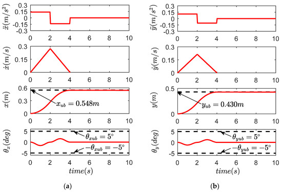
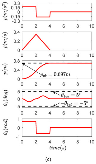
Figure 12.
Results for trajectory planning simulation. (a) X direction; (b) Y direction; (c) compound direction.
It can be seen from the simulation results that the trajectory planning strategy can quickly and accurately transfer the gantry and the trolley to the target position. The acceleration and speed are always within a limited range. The payload swing angle is always in the range of less than . After the trolley and gantry reach the target displacement, the payload does not have any residual swing.
7.4. Control Law Experimental Results and Analysis
To validate the actual performance of the proposed approach, three groups of experiments are implemented on the gantry crane test bench (see Figure 7). Specifically, we first compare the proposed scheme with the traditional energy based method. Then, the robustness of the proposed approach is tested by modifying the system parameters. At last, the proposed approach is further verified by taking into account the external perturbation. The system physical parameters are and , and the identifying locations are set to be and .
To be self-contained, we provide the expressions of energy-based controllers designed in the work of [10]. The gantry kinetic energy coupling control law (GKE) and the trolley kinetic energy coupling control law (TKE) are as follows:
Experiment 1.
Control performances validation with exact parameter information. In this experiment, the mass of the payload and the length of the rope are determined as
The control gains for the two control laws are fully tuned until the respective best performance is achieved, which are explicitly given in Table 2.
Table 2.
Control gain for experiment 1. GKE, gantry kinetic energy; TKE, trolley kinetic energy.
First, the gantry is transferred separately for 30 s in the X direction. Then, the trolley is transferred separately for 30 s in the Y direction. Finally, the trolley and the gantry are transferred for 30 s at the same time. The experimental results are shown in Figure 13 and Figure 14, and the quantified results are detailed in Table 3, which includes the following four performance indices: (1) that denotes the maximum swing amplitude during the transferring process; (2) payload residual swing , which refers to the maximum swing amplitude after the gantry and the trolley stop; (3) settling time , which is defined as the time when the swing angle enters the range of ; (4) maximum actuating force .

Figure 13.
Results for gantry kinetic energy (GKE) and trolley kinetic energy (TKE) in Experiment 1. (a) X direction; (b) Y direction; (c) compound direction.

Figure 14.
Results for proposed controller in Experiment 1. (a) X direction; (b) Y direction; (c) compound direction.
Table 3.
Control performance comparison for Experiment 1.
On the basis of the experiment results shown in Figure 13 and Figure 14 and Table 3, it is concluded that both control laws can transfer the gantry and trolley to the target position within 10 s. However, the transient response of the proposed controller (38) is superior over that of the other control law. Payload swing is much better suppressed and eliminated by the proposed control law. There is almost no residual swing when the granty and trolley reach the desired location.
Experiment 2.
Robustness verification experiment. Here, to test the robustness of the proposed control law (38) against parameter variations, we change the payload mass and rope length to distinguish them from corresponding nominal values. The actual parameters are decided as
The control gains for the control law (38) and (66) are kept the same as those in Experiment 1.
Figure 15 and Figure 16 show the results of Experiment 2, and the explicit quantified data are provided in Table 4. It is clear by comparing Figure 14 and Figure 16 that the performance of the proposed control law (38) is hardly influenced by the parameter changes in the sense that the transportation efficiency and payload suppression effect remain almost the same as those of Experiment 1. By contrast, the performance of the GKE and TKE control law (66) is largely degraded because of the fact that the model-dependent structures make them sensitive to parameter uncertainties, while in real-world applications, it is impossible to always know the exact values including rope lengths and payload masses; in this sense, the proposed method is more practical.
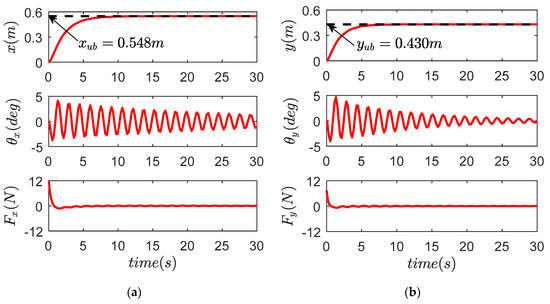
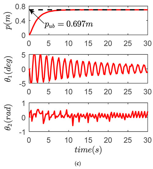
Figure 15.
Results for GKE and TKE in Experiment 2. (a) X direction; (b) Y direction; (c) compound direction.
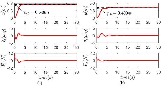
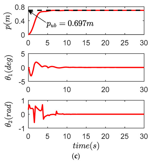
Figure 16.
Results for proposed controller in Experiment 2. (a) X direction; (b) Y direction; (c) compound direction.
Table 4.
Control performance comparison for Experiment 2.
Experiment 3.
To further verify its robustness against external perturbation, we examine the performance of the proposed controller (38) by using a wooden stick to strike the payload. The parameters including the control gains are chosen the same as those in Experiment 1.
First, the gantry is transferred separately for 30 s in the X direction. We use a wooden stick to strike the payload in the X direction at 20 s. Then, the trolley is transferred separately for 30 s in the Y direction. We use a wooden stick to strike the payload in the Y direction at 20 s. Finally, the trolley and the gantry are transferred for 30 s at the same time. We use a wooden stick to strike the payload in the compound direction at 20 s.
The experimental results are shown in Figure 17 and Figure 18 and Table 5. We can conclude that both control laws can act against external perturbation, but the transient response of the proposed controller (38) is superior over that of the other control law. Payload swing is much better suppressed and eliminated by the proposed control law when the payload meets the external perturbation.

Figure 17.
Results for GKE and TKE in Experiment 3. (a) X direction; (b) Y direction; (c) compound direction.
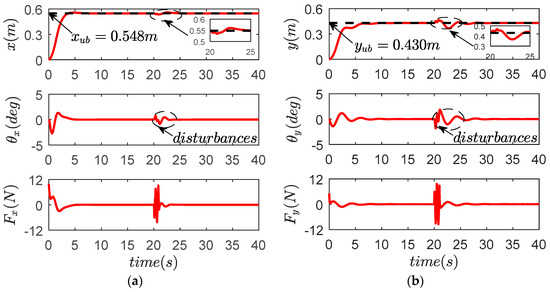
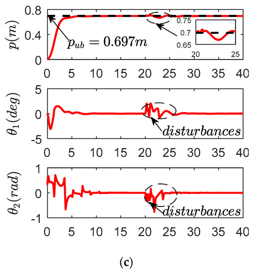
Figure 18.
Results for proposed controller in Experiment 3. (a) X direction; (b) Y direction; (c) compound direction.
Table 5.
Control performance comparison for Experiment 3.
8. Conclusions
Aiming at the symmetry underactuated gantry crane control system, this paper proposes a nonlinear control method of symmetry underactuated gantry crane based on machine vision positioning. The method detects the transfer target by the visual sensor and plans the trajectory, which improves the automation efficiency of the gantry crane. The designed control law not only makes the payload transfer to the target position accurately, but also effectively suppresses the payload swing and enhances the stability of the system in response to external disturbances. The proposed control law enhances the coupling behavior between the payload and the various state quantities of the gantry crane and leads to an improved control performance. Theoretical analysis and experimental results show that the proposed control method has good accuracy, stability, and rapidity for the symmetry underactuated gantry crane control system. Future work will focus on extending the proposed method to the overall-process control of gantry cranes with payload hoisting and lowering.
Author Contributions
Authors H.S. and G.L. conceived and designed the model for research, and analyzed the data and the obtained inference. Author J.H. performed the experiments. Authors X.B. and G.L. processed experimental data and wrote the paper. The final manuscript has been read and approved by all authors.
Funding
His research was funded by The National Key R & D Program of China, grant number 2017YFC0703903. The National Natural Science Foundation of China, grant number 51705341, 51675353.
Acknowledgments
The authors are grateful to the editors and the anonymous reviewers for providing us with insightful comments and suggestions throughout the revision process.
Conflicts of Interest
The authors declare no conflict of interest.
References
- Fang, Y.; Ma, B.; Wang, P.; Zhang, X. A Motion Planning-Based Adaptive Control Method for an Underactuated Crane System. IEEE Trans. Control Syst. Technol. 2012, 20, 241–248. [Google Scholar] [CrossRef]
- Pezeshki, S.; Badamchizadeh, M.A.; Ghiasi, A.R.; Ghaemi, S. Control of Overhead Crane System Using Adaptive Model-Free and Adaptive Fuzzy Sliding Mode Controllers. J. Control Autom. Electr. Syst. 2015, 26, 1–15. [Google Scholar]
- Sun, N.; Wu, Y.; Chen, H.; Fang, Y. An energy-optimal solution for transportation control of cranes with double pendulum dynamics: Design and experiments. Mech. Syst. Signal Process. 2018, 102, 87–101. [Google Scholar]
- Sun, N.; Yang, T.; Fang, Y.; Wu, Y.; Chen, H. Transportation Control of Double-Pendulum Cranes with a Nonlinear Quasi-PID Scheme: Design and Experiments. IEEE Trans. Syst. Man Cybern. Syst. 2019, 49, 1408–1418. [Google Scholar] [CrossRef]
- Lu, B.; Fang, Y.; Sun, N. Modeling and nonlinear coordination control for an underactuated dual overhead crane system. Automatica 2018, 91, 244–255. [Google Scholar]
- Yasir, M.; Ho, S.W.; Vellambi, B.N. Indoor Positioning System Using Visible Light and Accelerometer. J. Lightwave Technol. 2014, 32, 3306–3316. [Google Scholar] [CrossRef]
- Hossen, M.S.; Park, Y.; Kim, K.D. Performance improvement of indoor positioning using light-emitting diodes and an image sensor for light-emitting diode communication. Opt. Eng. 2015, 54, 035108. [Google Scholar]
- Truc, N.T.; Kim, Y.T. Navigation Method of the Transportation Robot Using Fuzzy Line Tracking and QR Code Recognition. Int. J. Hum. Robot. 2017, 14, 1650027. [Google Scholar]
- Moustafa, K.A.F.; Ebeid, A.M. Nonlinear modeling and control of overhead crane load sway. J. Dyn. Syst. Meas. Control 1988, 110, 266–271. [Google Scholar] [CrossRef]
- Fang, Y.; Dixon, W.E.; Dawson, D.M.; Zergeroglu, E. Nonlinear coupling control laws for an underactuated overhead crane system. IEEE/ASME Trans. Mechatron. 2003, 8, 418–423. [Google Scholar] [CrossRef]
- Tuan, L.A.; Kim, J.J.; Lee, S.G.; Lim, T.G.; Nho, L.C. Second-order sliding mode control of a 3D overhead crane with uncertain system parameters. Int. J. Precis. Eng. Manuf. 2014, 15, 811–819. [Google Scholar]
- Wu, X.; He, X. Partial feedback linearization control for 3-D underactuated overhead crane systems. ISA Trans. 2016, 65, 361–370. [Google Scholar]
- Zhang, M.; Ma, X.; Rong, X.; Song, R.; Tian, X.; Li, Y. An Enhanced Coupling Nonlinear Tracking Controller for Underactuated 3D Overhead Crane Systems. Asian J. Control 2018, 20, 1839–1854. [Google Scholar]
- Sun, N.; Fang, Y.; Zhang, Y.; Ma, B. A Novel Kinematic Coupling-Based Trajectory Planning Method for Overhead Cranes. IEEE/ASME Trans. Mechatron. 2012, 17, 166–173. [Google Scholar] [CrossRef]
- Makkar, C.; Hu, G.; Sawyer, W.G.; Dixon, W. Lyapunov-Based Tracking Control in the Presence of Uncertain Nonlinear Parameterizable Friction. IEEE Trans. Autom. Control 2007, 52, 1988–1994. [Google Scholar] [CrossRef]
- Di, Y.J.; Shi, J.P.; Mao, G.Y. A QR code identification technology in package auto-sorting system. Mod. Phys. Lett. B 2017, 31, 19–21. [Google Scholar]
- Canny, J. A Computational Approach to Edge Detection. IEEE Trans. Pattern Anal. Mach. Intell. 1986, PAMI–8, 679–698. [Google Scholar] [CrossRef]
- Kumar, G.; Umesh, G. Image steganography based on Canny edge detection, dilation operator and hybrid coding. J. Inf. Secur. Appl. 2018, 41, 41–51. [Google Scholar]
- Zhang, J.; Yu, H.; Deng, H.; Chai, Z.; Ma, M.; Zhong, X. A Robust and Rapid Camera Calibration Method by One Captured Image. IEEE Trans. Instrum. Meas. 2018, 1–10. [Google Scholar] [CrossRef]
- Li, J.; Liu, Z. Efficient camera self-calibration method for remote sensing photogrammetry. Opt. Express 2018, 26, 14213–14231. [Google Scholar] [PubMed]
- Kaehler, A.; Bradski, G. Learning OpenCV 3: Computer Vision in C++ with the OpenCV Library; O’Reilly Media: Sebastopol, CA, USA, 2016. [Google Scholar]
- Howse, J.; Joshi, P.; Beyeler, M. OpenCV: Computer Vision Projects with Python; Packt Publishing Limited: Birmingham, UK, 2017. [Google Scholar]
- Lee, H.H. Motion planning for three-dimensional overhead cranes with high-speed load hoisting. Int. J. Control 2005, 78, 875–886. [Google Scholar]
- Sun, N. Trajectory Planning and Nonlinear Control for Underactuated Cranes: Design, Analysis, and Applications. Ph.D. Thesis, Nankai University, Tianjin, China, 2014; pp. 19–56. [Google Scholar]
- Maghsoudi, M.J.; Mohamed, Z.; Sudin, S. An improved input shaping design for an efficient sway control of a nonlinear 3D overhead crane with friction. Mech. Syst. Signal Process. 2017, 92, 364–378. [Google Scholar] [CrossRef]
- Xie, X.; Huang, J.; Liang, Z. Vibration reduction for flexible systems by command smoothing. Mech. Syst. Signal Process. 2013, 39, 461–470. [Google Scholar]
- Uchiyama, N.; Ouyang, H.; Sano, S. Simple rotary crane dynamics modeling and open-loop control for residual load sway suppression by only horizontal boom motion. Mechatronics 2013, 23, 1223–1236. [Google Scholar] [CrossRef]
- Tuan, L.A.; Lee, S.G.; Ko, D.H.; Nho, L.C. Combined control with sliding mode and partial feedback linearization for 3D overhead cranes. Int. J. Robust Nonlinear Control 2014, 24, 3372–3386. [Google Scholar]
- Yu, W.; Li, X.; Panuncio, F. Stable Neural Pid Anti-Swing Control For An Overhead Crane. Intell. Autom. Soft Comput. 2014, 20, 145–158. [Google Scholar] [CrossRef]
- Khalil, H. Nonlinear Systems, 3rd ed.; Prentice-Hall: Englewood Cliffs, NJ, USA, 2002. [Google Scholar]


© 2019 by the authors. Licensee MDPI, Basel, Switzerland. This article is an open access article distributed under the terms and conditions of the Creative Commons Attribution (CC BY) license (http://creativecommons.org/licenses/by/4.0/).