Article

Column Generation Accelerated Algorithm and Optimisation for a High-Speed Railway Train Timetabling Problem

School of Traffic and Transportation, Beijing Jiaotong University, Beijing 100044, China
*
Author to whom correspondence should be addressed.
Symmetry 2019, 11(8), 983; https://doi.org/10.3390/sym11080983
Submission received: 19 June 2019 / Revised: 19 July 2019 / Accepted: 22 July 2019 / Published: 2 August 2019

Abstract

:
With the rapid development of high-speed railway (HSR) systems, the increasing demand for passenger traffic has put forward higher requirements for HSR train timetabling problems (HSRTTPs). This paper establishes two mathematical optimisation models with different optimisation objectives for an HSRTTP and solves these models through a column generation-based algorithm. However, the column generation-based algorithm has the disadvantage of a slow convergence rate, thus we put forward corresponding acceleration strategies for five stages of the algorithm: preprocessing, restricted master problem, pricing problem, branch-and-bound and postprocessing from a symmetry point between the computation efficiency and the accuracy. The effectiveness of the acceleration strategies was validated by a case study of the Beijing–Shanghai HSR. The results show that the proposed optimal acceleration strategies can increase the computation efficiency of the algorithm by 11.8× on average while ensuring the accuracy.

Graphical Abstract

1. Introduction

In 2018, the total volume of passenger flow in China was 17.9 billion, which was 30% higher than that in 1998 according to the National Bureau of Statistics of China. The increasing passenger travel demands have brought great pressure to the whole public transit systems. The proper management and better performance of public transit systems are effective ways to solve this problem [1,2,3,4,5,6,7]. As a low-carbon and environment-friendly public transit mode, high-speed railway (HSR) has developed rapidly in recent years, and its high speed and high density have made it the first choice for more and more passengers traveling between cities. As an important technical document of HSR systems, the train timetable is an important means to coordinate railway capacity and passenger demands. In recent years, more and more scholars pay attention to the HSR train timetabling problems (HSRTTPs). Niu et al. [8] established a non-linear integer programming model aimed at minimising the waiting times of passengers and studied the optimisation of train timetables based on time-varying passenger demands. Yue et al. [9] established an optimisation model of train timetables based on a space-time network to simultaneously consider both passenger demands and train scheduling. Zhou et al. [10] proposed a space-time-speed network modelling approach to achieve the joint optimisation of high-speed train timetables and speed profiles. A dynamic programming solution algorithm with a Lagrangian relaxation-based solution framework was applied to deal with the safety and power supply constraints. Jiang et al. [11] studied the problem of increasing the number of scheduled trains in a highly congested railway corridor to meet increasing passenger demands. The train timetabling problem (TTP) was NP-hard. Many scholars have proposed various effective approaches, such as the backtracking search [12], stochastic programming algorithm [13], train timetable simulation [14], sequencing optimisation algorithm [15] and Lagrangian relaxation algorithm [16]. The column generation algorithm is a common approach used for solving large-scale linear programming problems and has been successfully applied to the study of TTPs [9,17,18,19]. The idea of the column generation algorithm is that not all variables are enumerated for large-scale linear programming problems, and only the restricted master problem (RMP) composed of the subset of variables of the original problem is solved. The reduced cost of a variable with respect to the dual prices obtained by solving the RMP is used to find new variables that can improve the objective function or to test whether the original problem is optimal, which is called the pricing problem (PP). The new variables generated by the PP are added to the RMP, and then the new RMP is solved. The above steps are repeated until no new variable can be found. However, the column generation algorithm has some shortcomings, such as easy degeneration and difficulty acquiring integer solutions. In view of the existing problems of the column generation algorithm, He et al. [17] put forward the concept of a time interval path. After obtaining new columns by the PP, a heuristic column generation rule was used to enrich the neighbourhood of iteration, and this approach avoided the problem of easy degeneration to a certain extent. Chen and Shen [20] proposed a column removal strategy, strong label cutting rule and shift pool acceleration strategy for the application of a column generation-based algorithm in crew problems, and this approach had a significant effect in controlling the scale of the RMP, improving the solution speed of the PP and reducing the time required for finding an integer solution. Desaulners et al. [21] summarised the application of acceleration column generation algorithms in crew scheduling problems and vehicle routing problems. Gamache et al. [22] solved a scheduling problem in air transportation by using a column generation algorithm and proposed an early branching strategy to solve the easy degeneration problem of the column generation algorithm. A constrained branching strategy has a significant effect on improving the slow speed of finding integer solutions in the column generation algorithm [23,24,25,26,27], especially for the set partitioning problem and the set covering problem, but branching failure easily occurs when this strategy is applied in a set covering problem [20].
In this paper, two optimisation models for an HSRTTP are established by using a space-time network method. The first model aims to minimise the total number of train stops and stopping time from the perspective of meeting passenger demands and train scheduling. The second model aims to maximise the total number of trains from the perspective of maximising the physical capacity of the HSR line. We use a column generation-based algorithm to solve the above models. In view of the slow running speed of the algorithm, nine acceleration strategies are proposed based on the symmetry of efficiency and accuracy, namely arc elimination, column management, initial solution iteration, partial pricing, multiple paths, delayed constraint, early branching, column replacement and neighbourhood searching. In addition, the accuracy and effectiveness of the acceleration strategies are analysed using practical examples.
The remainder of this paper is organised as follows. In Section 2, the construction of the space-time network is introduced, and two optimisation models for train timetables are established. In Section 3, the column generation-based algorithm is discussed. In Section 4, the acceleration strategies for the column generation-based algorithm are elaborated. In Section 5, the effectiveness of the proposed acceleration strategies is verified based on data from the Beijing–Shanghai HSR. In Section 6, the conclusions and recommendations for future research are discussed.

2. Problem Formulation

2.1. Problem Description

The TTP can be described as follows. Given a train service plan, on the premise of meeting minimum headway constraints, with maximising the benefit of transport enterprises or minimising passenger travel costs as the optimisation objective, the train travel time in each section and the arrival or departure time of each station are arranged. In this paper, a space-time network is used to describe the TTP. A space-time network associates a railway network with time and discretises physical stations into several space-time network nodes parallel to the timer shaft, and these nodes can be used to describe the events happening at different times for the physical stations [17]. To ensure that a train meets the network flow constraints, a unified virtual departure node and virtual arrival node are set up. The space-time network starts from the virtual departure node. The virtual departure arc represents the train’s feasible departure time, and the virtual arrival arc represents the train’s feasible arrival time. The train’s feasible departure time can be determined according to the train service plan. The section connection arc is used to describe the train travel time of the section and the additional starting and stopping time. The station passing arc and station dwell arc are used to describe the passing, arrival and departure times of the train in a station. The train dwell time at the station should meet the requirements of the maximum and minimum dwell times [19]. The maximum dwell time is set to control the scale of the space-time network, and the minimum dwell time is the minimum time required for passenger boarding, alighting, transferring and other behaviours. The network ends at the virtual arrival node. All generated space-time nodes and space-time arcs jointly constitute the feasible path set of the trains. The train timetable allocates a space-time path for each train in turn from the feasible path set under the conditions of satisfying several constraints, such as the departure safety headway constraints, the arrival safety headway constraints and the station capacity constraints. We define a “cost” for each path to evaluate the quality of the train timetable. In the TTP, the number of trains, travel time, departure time, arrival time, number of stops and stopping time are all important parameters. The incorporation of more trains produces a greater effective trafficability of the train timetable, meaning that it can undertake more passenger transport tasks. For passengers, when the departure and arrival times are acceptable, the appropriate travel time, which is affected by the number of train stops and the stopping time, is an important factor in their choice of HSR as a means of travel, and the HSR system also needs to provide a sufficient number of trains to meet passenger demands. The total number of trains required for each origin-to-destination (OD) pair on a railway line to satisfy the passenger demand can be determined by analysing the passenger flow OD matrix [9]. Therefore, the cost of a path defined in this paper is related to the travel time, the number of train stops, the stopping time and the number of trains.
Figure 1 depicts the relationships among the railway network, train timetable and space-time network. One railway line consists of four stations and three sections. The train timetable describes the space-time information of four trains running on the line. At a certain time, Train A travels from Station S2 to Station S3, Train B travels from Station S1 to Station S2 and Train C stops at Station S3. This information can be accurately described by the train timetable and the space-time network diagram, and the train trajectory in the train timetable corresponds to a feasible path in the space-time network (as shown by the blue bold path in Figure 1).

2.2. Notation

Table 1 lists the general subscripts, sets and input parameters used in the mathematical formulations, where the unit of time is one minute.

2.3. Mathematical Model

The 0–1 decision variable x p ( p P j ) is used to express whether the space-time path p is selected by the train j . In consideration of passenger demands, some stations can be set as adjustable stations; that is, trains are allowed to choose whether to pass or stop at these stations. In the space-time network, the paths are allowed to generate both passing arcs and dwell arcs at these stations, but the OD service frequency requirements given by the train service plan should be satisfied. If all stations are set as adjustable stations, this creates a problem for the integrated optimisation of stopping patterns and train timetables. The optimisation model for the HSRTTP based on passenger demands is established as follows.
M1:
z 1 = min p P x p c p 1 = min p P i : u p i = 1 x p [ β 1 + β 2 ( t p , i end t p , i beg ) ] .
p P j x p = 1 j N .
x p + x p 1 e E , p , p P e : 0 t p , e dep t p , e dep < t e dep .
x p + x p 1 e E , p , p P e : 0 t p , e arr t p , e arr < t e arr .
x p + x p 1 e E , p , p P e : ( t p , e dep t p , e dep ) ( t p , e arr t p , e arr ) 0 .
p P : t p , i beg t , t p , i end t x p n i i S , t T .
p P : τ p i , i = 1 x p v i , i i , i S , i i .
v i , i = Q i , i φ ω i , i i , i S , i i .
t i min t p , i end t p , i beg t i max   i S , p P : u p i = 1 .
x p = { 0 , 1 }   p P .
The objective function in Equation (1) expresses that the total number of stops and the total stopping times of trains are minimised. The constraints in Equation (2) are network flow constraints that express that each train selects and can only select one path in the space-time network. The constraints in Equation (3) express that the departure times of adjacent trains moving in the same direction in the same station must be greater than or equal to the minimum departure headway. The constraints in Equation (4) express that the arrival times of adjacent trains in the same direction in the same station must be greater than or equal to the minimum arrival headway. The constraints in Equation (5) express that trains moving in the same direction are not allowed to intersect within a section and that trains can only overtake at stations. The constraints in Equation (6) express that the number of trains stopping or passing at the same station at the same time cannot exceed the number of sidetracks available at the station, and the upward and downward directions should be distinguished in the calculation. The constraints in Equation (7) express that the number of trains served in each OD pair should meet the OD service frequency given by the train service plan. The constraints in Equation (8) are the conversion relationships between OD service frequencies and the passenger flow OD matrix. The constraints in Equation (9) express that the stopping times of trains at parking stations should meet the requirements of the minimum and maximum dwell times. The constraints in Equation (10) are the value constraints of the decision variables.
The objective function of Model M1 is replaced by Equation (11), and the constraints in Equation (2) are relaxed to the constraints in Equation (12). The optimisation model for the HSRTTP based on maximum utilisation of the physical capacity of the railway line is established as follows.
M2:
z 2 = max p P x p c p 2 = max p P x p .
s.t. (3)–(10).
p P j x p 1 j N .
The objective function in Equation (11) expresses that the number of trains is the maximum. The constraints in Equation (12) express that each train meeting the constraints of Model M2 selects and only selects one path in the space-time network and those that do not meet the constraints are not arranged.

3. Column Generation-Based Algorithm

Models M1 and M2 are both 0–1 integer programming models. A column generation algorithm and branch-and-bound algorithm are combined to solve the models in this paper. We use the space-time network to describe the HSRTTP to construct a 0–1 integer programming model based on the network flow, and each path in the space-time network corresponds to a full timetable for a train. However, with the increase of the number of stations and trains of the TTP, the space-time network will generate many space-time arcs and nodes, resulting in much more feasible path variables. The column generation algorithm is one of the effective methods for solving large-scale linear programming problems in which the number of variables is much larger than the number of constraints. Combined with the branch-and-bound algorithm, the HSRTTP based on the space-time network can be effectively solved. The column generation algorithm is used to solve the linear relaxation problem of each node in the branch tree and to obtain the lower bound (LB) of the original problem. The branch-and-bound method is used to solve the integer programming problem and to obtain the upper bound (UB) of the original problem. The optimal solution of the original problem is obtained by continually iterating the upper and lower bounds.

3.1. Column Generation Algorithm

We relax the integer decision variable x p = { 0 , 1 } to a continuous variable 0 x p 1 and take a subset P 0 P to form the RMP. Equation (9) is mainly used for the construction of a space-time network and is not considered here. The RMP can be solved by some commercial computing software packages, and the obtained solution and dual variables can be used to calculate the PP.
γ j , δ e , p , p , ϕ e , p , p , η e , p , p , λ i , t , θ i , i are defined as the dual variables of Equations (2)–(7), respectively. For Models M1 and M2, the reduced cost of any one path p P j in the space-time network is calculated as follows.
ξ p 1 , 2 = c p 1 , 2 γ j e E p P e p P e δ e , p , p e E p P e p P e ϕ e , p , p e E p P e p P e η e , p , p i S t T λ i , t i S i S θ i , i .
The original problem is transformed into corresponding sub-problems according to the number of trains. The PP updates the weights of the space-time arcs by using the dual variables obtained from solving the RMP and then finds the shortest (minimum reduced cost) path among these sub-problems. As shown in Equation (14), the path with the minimum reduced cost ξ min is added to the RMP to continue the iterative computation. If a path with a reduced cost of less than 0 cannot be found in an iteration, the optimal solution can be obtained.
ξ min = arg min { ξ p | ξ p < 0 , p P P 0 } .
For Models M1 and M2, because the dual variables of Equation (7) are related to any two different parking stations on the line, these dual variables cannot be updated directly to specific arcs, so the commonly used shortest path algorithms are not applicable. Therefore, we propose an algorithm based on the A-star algorithm and the shortest path faster algorithm [19] to solve the above problems. Model M2 can also be used to calculate the initial feasible solution of Model M1. The train information in Model M2 is given by the train service plan, including the total number of trains, types of trains, departure stations, arrival stations, stopping patterns and other information. Original trains can be generated randomly according to the train information as the initial feasible solution and added to Model M2. Then, the column generation-based algorithm is used for the calculation, and the obtained integer optimal solution can be used as an initial feasible solution of Model M1.

3.2. Branching Strategies

At present, the commonly used branching strategies are the constraint-based branching strategy and variable-based branching strategy, also known as the fast branching strategy. The former is mainly applicable to set covering models and set partitioning models, which are often used to solve problems of crew scheduling and vehicle routing. However, this method has the possibility of branching failure for a set covering model [20]. The fast branching strategy consists of partitioning the space of solutions by forcing the branch variables to 0 or 1 and adding them into the constraints. The meaning of branch 0 is to specify that a train does not choose a certain path, which is equivalent to solving the k shortest path problem in the corresponding sub-problem. The computation is relatively time consuming and has little significance for solving the problem. Therefore, we usually choose only branch 1, that is, a train is designated to select a certain path. Beam search [28] and depth-first search algorithms are combined for branching, and a fixed number of fractional solutions are selected as branch nodes to join in the branch tree each time according to the ordering rule, where the fractional solutions are sorted from largest to smallest according to the values calculated from the formula c p min { x p , 1 x p } . The nodes in the branch tree are sorted from largest to smallest according to the node layers.
ε refers to the stopping criterion of the algorithm, A refers to the active branch node set, B w ( w A ) refers to the variable set to be branched corresponding to active branch node w , C w ( w A ) refers to the variable set branched corresponding to w , and G min refers to the new calculated shortest path set. Therefore, the steps of the column generation-based algorithm to solve the optimization problem of the HSRTTP are as follows.
Step 1
Construct a space-time network. Generate an initial path set P 0 as the root node of the branch tree and add it to A . Set U B = + and L B = - .
Step 2
Judge whether A is an empty set. If it is, the algorithm stops; otherwise, go to Step 3.
Step 3
Judge whether ( U B L B ) / U B ε is true or not. If it is true, the algorithm stops; otherwise, go to Step 4.
Step 4
Judge whether the minimum objective function value of the nodes in A is greater than L B . If it is, update L B . Sort A according to the depth-first strategy, select the first node w , and remove it from A . Judge whether node w is the root node. If it is, go to Step 6; otherwise, go to Step 5.
Step 5
Judge whether B w of node w is empty. If it is, go to Step 2; otherwise, the first variable k 0 to be branched is selected from B w and added to C w . Each branch variable k in C w is circulated, and x k = 1 is added to the model as the constraint. Remove k 0 from B w , and go to Step 6.
Step 6
The column generation algorithm is used to solve the linear relaxation problem of node w .
Step 6.1
The initial feasible solution of the RMP is generated. Suppose that G min = .
Step 6.2
The dual variables are obtained by solving the RMP. If an integer solution is obtained and is less than U B , update U B .
Step 6.3
The dual variables are used to update the weights of the space-time arcs and calculate the shortest path of each sub-problem. The path satisfying the requirement of reduced cost ξ p is added to set G min .
Step 6.4
Judge whether G min is empty. If it is, go to Step 7; otherwise, add the paths in G min to the RMP. Remove the paths from G min , and go to Step 6.2.
Step 7
Judge whether the objective function of w is less than U B . If it is, the new active node w is added to A , C w is added to C w , the fractional variables in the results are sorted according to certain rules, and a certain number of variables are selected and added to B w according to the beam search algorithm. Delete the variable k from B w , and go to Step 5. Otherwise, pruning is conducted, and the variable k 0 is deleted from C w . Then, go to Step 5.

4. Acceleration Strategies of the Column Generation-Based Algorithm

We propose acceleration strategies for each of the five phases of preprocessing, RMP, PP, branch-and-bound and postprocessing to solve the mathematical models.

4.1. Preprocessing Stage

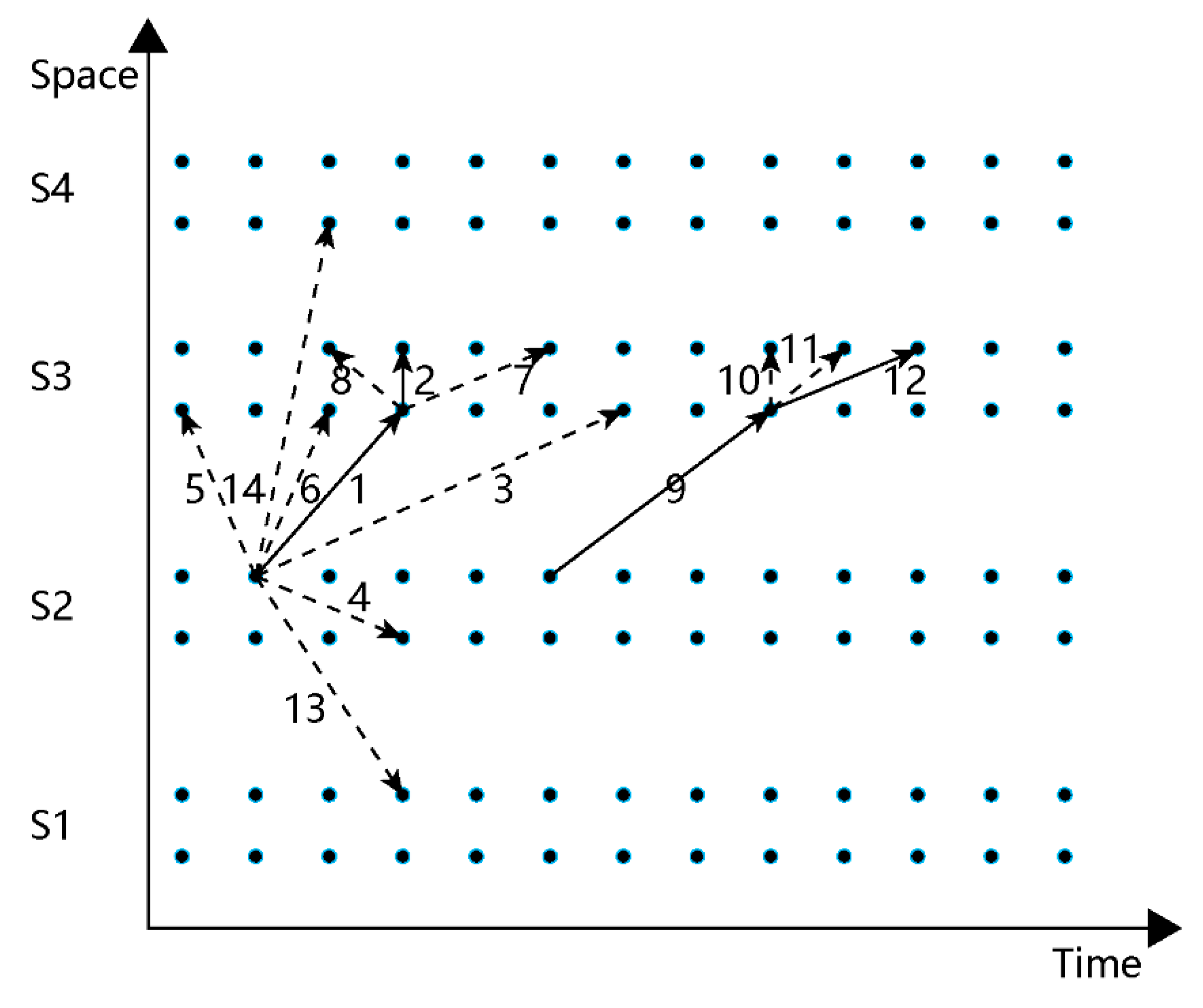
The acceleration strategy in the preprocessing stage is the arc elimination strategy, which is mainly applied to eliminate redundant arcs according to the train service plan and actual situation [9]. It can reduce the network size and solution space in the construction of the space-time network. As shown in Figure 2, each space-time node in the space-time network can be connected by many arcs, including section connection Arcs 1, 3, 5, 6, 9, 13, and 14; station passing Arcs 2 and 10; and station dwelling Arcs 7, 8, 11, and 12, among which Arcs 1, 2, 9, and 12 are feasible. Arcs 3 and 6 do not accord with the running time in the section; Arc 4 does not accord with the train running direction; Arcs 5 and 8 do not accord with the time direction; Arcs 13 and 14 do not accord with the variable definitions; and Arc 11 does not meet the minimum dwell time requirement of the station. If Arc 1 is selected, Arc 7 does not conform because Arc 1 passes through Station S3, and a dwell arc should not be connected. Similarly, if Arc 9 is selected, Arc 10 does not conform because Arc 9 stops at Station S3, and a passing arc should not be connected. Through the above methods, redundant arcs can be effectively eliminated so that the search space of the feasible paths of trains is controllable.

4.2. RMP Stage

4.2.1. Column Management Strategy

As the number of iterations increases, the size of the RMP will become larger, and the solving time will be longer. To solve this problem, a column management strategy is designed here. When the number of paths in the RMP exceeds a certain criterion n C M S , the paths that perform poorly, that is, those whose reduced cost exceeds a certain criterion, ϑ C M S , are eliminated. However, because the reduced cost of a path changes with the iteration progress, some poorly performing paths may be transformed into paths that meet the requirements, so only removing the paths is not appropriate. Therefore, a column management pool (CMP) is designed, and the removed paths can be added to the CMP. In each iteration, the paths in the CMP are computed first, and the paths meeting the requirements are added to the RMP. If the reduced cost of a path in the CMP exceeds ϑ C M S for 10 consecutive iterations, that path will be removed from the CMP.

4.2.2. Initial Solution Iteration Strategy

To control the size of the RMP, an initial solution iteration strategy is proposed. Using the integer solutions that are superior to the current upper bound value as the new initial feasible solutions, the whole algorithm is re-operated from the root node, and this strategy not only improves the operation efficiency but also effectively controls the size of the problem. In practical computation, a better integer solution I 0 should be compared to the upper and lower bounds of the original problem after being obtained. Equation (15) and the criterion ϑ I I S should be satisfied before the initial solution iteration is carried out to avoid excessive time consumption due to frequently solving the linear relaxation problem of the root node.
U B I 0 I 0 L B ϑ I I S .

4.3. PP Stage

4.3.1. Partial Pricing Strategy

In a traditional column generation method, each time the PP is solved, all the sub-problems are computed in turn, and the new path with the minimum reduced cost is added to the RMP. The advantage of this method is that the path that most improves the objective function is produced in each iteration, but using the same dual variables in all sub-problems will lead the produced columns to cover the same arcs. If solving the sub-problems becomes more complex, the computation time will be prolonged.
A feasible method is to calculate only a fixed number m ( m < l ) of sub-problems each time the PP is solved. First, all sub-problems are numbered before computation begins. Each time the PP is solved, m sub-problems are calculated in numerical order, and the newly generated path with a reduced cost of less than 0 and the minimum is added to the RMP. The next iteration starts at the end of the last iteration. If there is no path that meets the requirements after m sub-problems are computed, the remaining sub-problems continue to be computed until one path that meets the requirements is produced. Although this method leads to an increase in the number of iterations, the computation time of each iteration is reduced accordingly.

4.3.2. Multiple Paths Strategy

Because the column generation algorithm does not necessarily require the path with the minimum reduced cost, as long as the reduced cost of the path is less than 0, the objective function can be improved. If the large number of sub-problems leads to a long computation time of the PP and adding only one path with a minimum reduced cost in each iteration may not achieve the desired effect, multiple paths meeting the reduced cost requirement can be added in each iteration according to certain rules. Goffin and Vial [29] proved the effectiveness of this strategy. However, it should also be noted that, if too many paths are added to each iteration, the size of the RMP will become increasingly larger, and the solving time will be prolonged accordingly.

4.3.3. Delayed Constraint Strategy

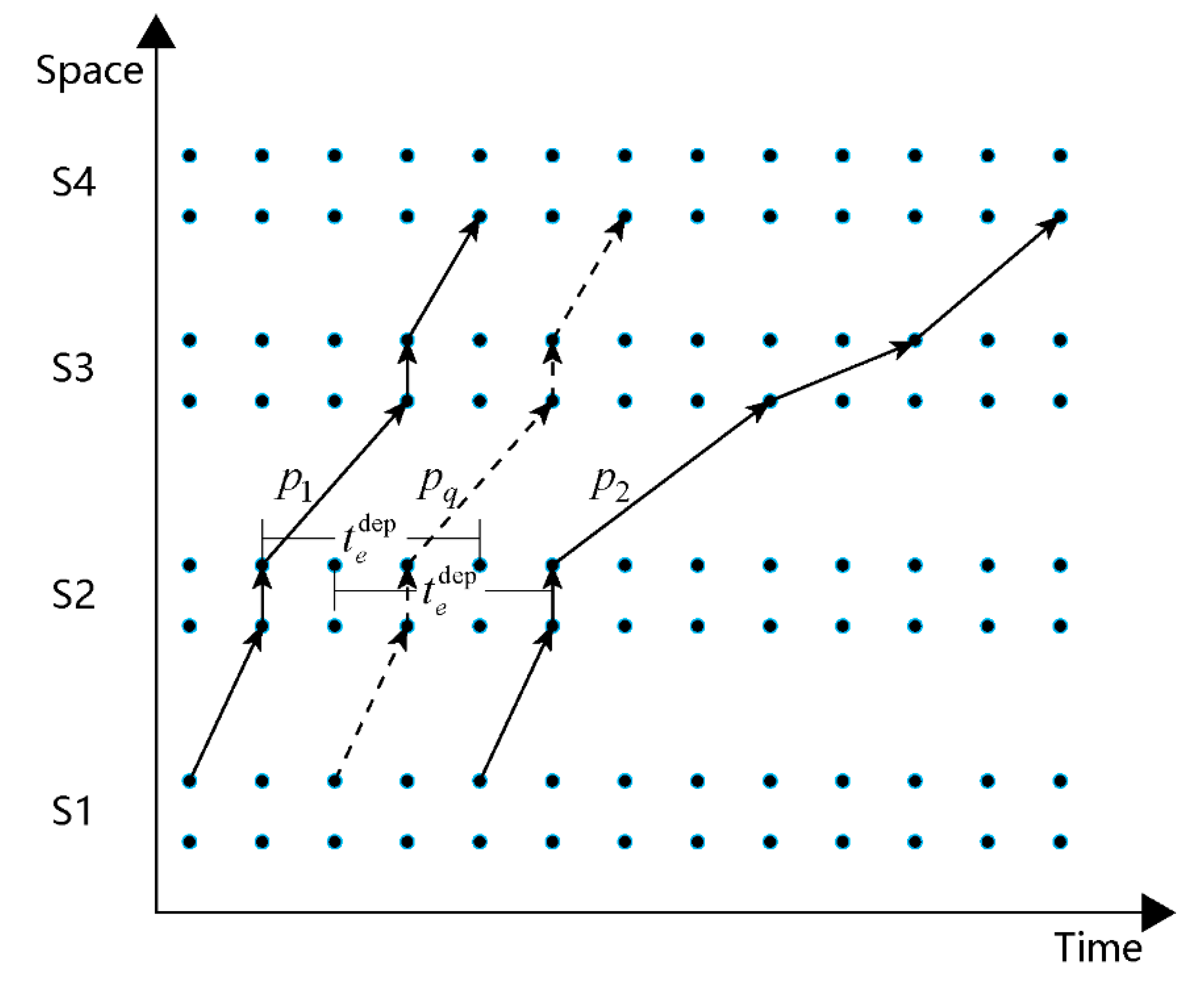
It is not difficult to find from the actual computation that adding the paths from the PP solution to the RMP cannot desirably improve the objective function. The reason is that newly added path variables have relatively small values and can even be 0. This phenomenon is caused by the conflicts between the newly added paths and the paths in the RMP. Figure 3 depicts this problem. Currently, the RMP has paths p 1 and p 2 , between which there are no conflicts and which do not conflict with other paths in the RMP. Using the constraints in Equation (3) as examples, the dual variables of both paths in the section e which is from Station S2 to Station S3 are 0. Therefore, the weight of each departure arc at Station S2 in the time range [ t p 1 , e dep , t p 1 , e dep + t e dep ) is not affected by path p 1 . Suppose that path p q is a path selected by the PP and added to the RMP. According to Equation (3), path p q must satisfy the constraints x p 1 + x p q 1 and x p q + x p 2 1 , which may result in the variable value of path p q being less than 1 or even 0, so that the newly added path may not achieve the desired role in reducing the value of the objective function. The constraints in Equation (4)–(6) are similar to the constraints in Equation (3). Such constraints are called delayed constraints; that is, the effect of the current constraints may be shifted to the next iteration. To solve the problem of delayed constraints, a delayed weight attribute is attached to each space-time arc. In the process of the PP updating the space-time network, the average values of the path variables in recent iterations can be used to update the delayed weights of the corresponding arcs.

4.4. Branch-and-Bound Stage

4.4.1. Early Branching Strategy

In the initial iteration stage, the objective function of the column generation algorithm changes greatly, and the convergence rate is relatively fast. However, at the end of the iteration, the objective function changes less with increasing numbers of iterations. This is called the easy degeneration phenomenon, which appears in the process of solving the nodes of the whole branch-and-bound tree and seriously affects the efficiency. This phenomenon is also a significant shortcoming of column generation algorithms.
At present, a feasible method is the early branching strategy [22]. When the change rate of the value of the objective function within a certain number of iterations n E B S does not exceed a specified criterion ϑ E B S , the current iteration process is terminated in advance, and the branching strategy is started directly. Although the current algorithm has not achieved convergence, experiments show that this method can achieve convergence in the subsequent branching process and can effectively avoid easy degeneration of the column generation algorithm. v r is denoted as the objective function value produced in the current iteration, and Equation (16) is used to judge whether the early branching strategy needs to be started.
v r n E B S + 1 v r v r n E B S + 1 < ϑ E B S .

4.4.2. Column Replacement Strategy

A column replacement strategy is used in branching processes. Each time branching occurs, the algorithm specifies a certain train j to choose a path p ( p P j ) according to the constraints. When dual variables of path p are used to update the arc weights, all the arcs in the space-time network that conflict with path p are not available. We denote the weights of these arcs as + . When the shortest path problem is calculated, the paths passing through these arcs can be directly ignored, which is conducive to reducing the size of the problem. Additionally, because of the existence of branching constraints, all the values of path variables in the current branch node conflicting with these constraints are 0, which may lead to the RMP having no feasible solution and the branch being pruned, thus affecting the balance of the branch tree.
At this point, the column replacement strategy can be adopted; that is, a feasible path covering the same train with the conflict path in the space-time network is added to the RMP to replace the conflict path. When this feasible path is selected, the specific arcs that conflict with the branch constraints can be moved, or the whole path in the feasible range can be moved by translation until there is no conflict with the branching constraints. Finally, the conflicting path is replaced with the newly generated path.

4.5. Postprocessing Stage

We propose a neighbourhood search strategy to generate a new path based on the path obtained by solving the PP, and add the generated path to the RMP to avoid easy degeneration of the column generation algorithm. The specific method is to find the paths that neighbour and have the same reduced cost as that of the path generated by the PP, and these paths are added to the alternative set. Combined with the delayed constraint strategy, the delayed weight attribute is added to the reduced cost of each arc. The paths in the alternative set are sorted according to the reduced cost, and the path with the minimum reduced cost is selected to replace the original path to be added to the RMP. The delayed constraint strategy can effectively avoid conflicts between the newly added paths and the original paths in the RMP so that the newly added paths can better improve the objective function. Additionally, if the delayed weight attribute of each arc is calculated in the PP, the search time of the shortest path will be prolonged, but this problem can be effectively avoided by applying the neighbourhood search strategy.

5. Case Study

We considered the Beijing–Shanghai HSR to verify the effectiveness and efficiency of the column generation-based algorithm. The code was written in C#, and the solution of the RMP used CPLEX 12.7.1 with its default parameters as the solver. The algorithm was deployed on a desktop computer with the Windows 10 operating system, an AMD 2400G 3.6 GHz processor and 16 GB memory. In the experimental results, all units of time are in seconds.
As shown in Figure 4, the length of the Beijing–Shanghai HSR is 1302 km, and there are 23 stations along the corridor. As of 30 June 2018, the Beijing–Shanghai HSR had served 825 million passengers. All trains running in the corridor were classified as two speed classes, Grade G (300 km/h) and Grade D (250 km/h), in 2016. Because of the time designated for maintenance and testing, our research time is from 06:30 to 00:00 [9].
Table 2 lists the station names in the Beijing–Shanghai HSR and the number of tracks in each station. Table 3 lists the data of the section travel time.
The calculations were performed with trains travelling in the downward direction as an example. Table 4 lists the OD service frequency data for the downward direction. The values of the parameters t e dep , t e arr , t i min , t i max , β 1 G , β 2 G , β 1 D , β 2 D , ε , n C M S , ϑ C M S , ϑ I I S , n E B S , and ϑ E B S were set to 2 min, 3 min, 2 min, 8 min, 2, 2, 1, 1, 0.18, 10, 0, 0.33, 12, and 0.05, respectively.
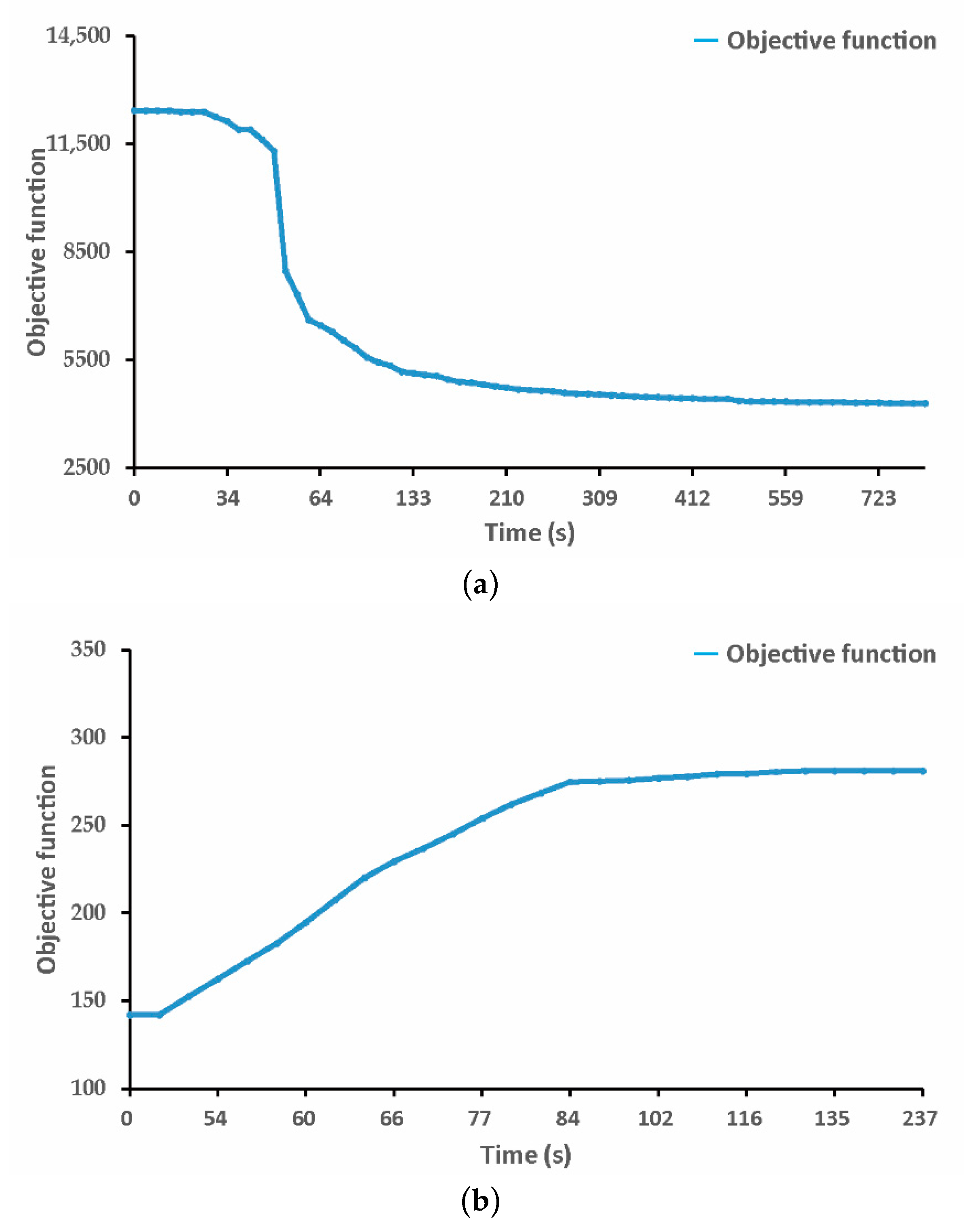
Figure 5 shows the iterative process of the column generation-based algorithm when used to solve the linear relaxation problem of the root node of Models M1 and M2. As shown in Figure 5, with increasing calculation time, the objective functions of the models all rapidly change and gradually converge.
Table 5 summarizes the comparisons of the actual train timetable for the Beijing–Shanghai HSR in May 2016, a train timetable calculated using Model M1 and a train timetable calculated using Model M2 in terms of the average travel speed, the average number of stops at stations, and the average station dwell time.
As shown in Table 5, upon comparing the actual train timetable and the train timetable calculated using Model M1, the total number of train stops, the total stopping time and the number of occurrences of overtaking are reduced by 46%, 58% and 69%, respectively, and the average travel speed is improved by 10.2%. Upon comparing the actual train timetable and the train timetable derived using Model M2, the number of trains is greatly improved, with an increase of 41%. These results indicate that our proposed models and algorithm can effectively improve the quality of a constructed train timetable and the travel efficiency for passengers.
Table 6 shows five instances designed for the Beijing–Shanghai HSR, in which “Y” represents that the station is an adjustable station and “N” represents that the station is an unadjustable station, where the train stops or passes according to the given stopping patterns. Instances 1–3 are designed for Model M1. Some stations are set as adjustable stations to test the efficiency of the algorithm under different stopping patterns. Additionally, the changed stopping patterns also need to meet the OD service frequency. Instance 3 sets all the intermediate stations as adjustable stations, and this example can be regarded as the problem for integrated optimization of the stopping pattern and train timetable based on the passenger service demands. Instances 4–5 are designed for Model M2.
The following is a detailed test of the acceleration strategies for the proposed column generation-based algorithm.
Table 7 presents comparisons of the calculation times and Gap values for the following five cases:
Case 1
A train timetable calculated using the original column generation-based algorithm.
Case 2
A train timetable calculated using the improved column generation-based algorithm with the acceleration strategies of the column management strategy and initial solution iteration strategy.
Case 3
A train timetable calculated using the improved column generation-based algorithm with the acceleration strategies of the early branching strategy and column replacement strategy.
Case 4
A train timetable calculated using the improved column generation-based algorithm with the acceleration strategies of the delayed constraint strategy and neighbourhood search strategy.
Case 5
A train timetable calculated using the improved column generation-based algorithm with all nine acceleration strategies.
The Gap value refers to the degree of deviation of the upper and lower bounds of the problem and is calculated by G a p = ( U B L B ) / U B . Table 7 shows that the acceleration strategies proposed in this paper can effectively improve the efficiency of the column generation-based algorithm on the basis of guaranteeing accuracy. The target value of Gap was set to 0.18 and the maximum number of iterations was set to 3000. The optimal strategy tested in Case 5 has the best effect. Compared with the original column generation-based method, this strategy can increase the efficiency of the algorithm by 11.8× on average and reduce the Gap value by 56% on average. The delayed constraint strategy and neighbourhood search strategy tested in Case 4 also exhibit relatively good performances, which can minimize the conflicts between the newly added paths and the paths in the RMP and enhance the effect of the new paths to improve the objective function. The computation result of Case 1 is worse than that of the optimal strategies because the algorithm consumes more time in solving integer solutions. The strategies tested in Cases 2 and 3 have a certain effect on the efficiency of the column generation-based algorithm. On the one hand, the limited effects of these strategies are due to the parameter settings, and, on the other hand, the effect of the newly added paths is not very obvious due to the loss of the delayed constraint strategy.
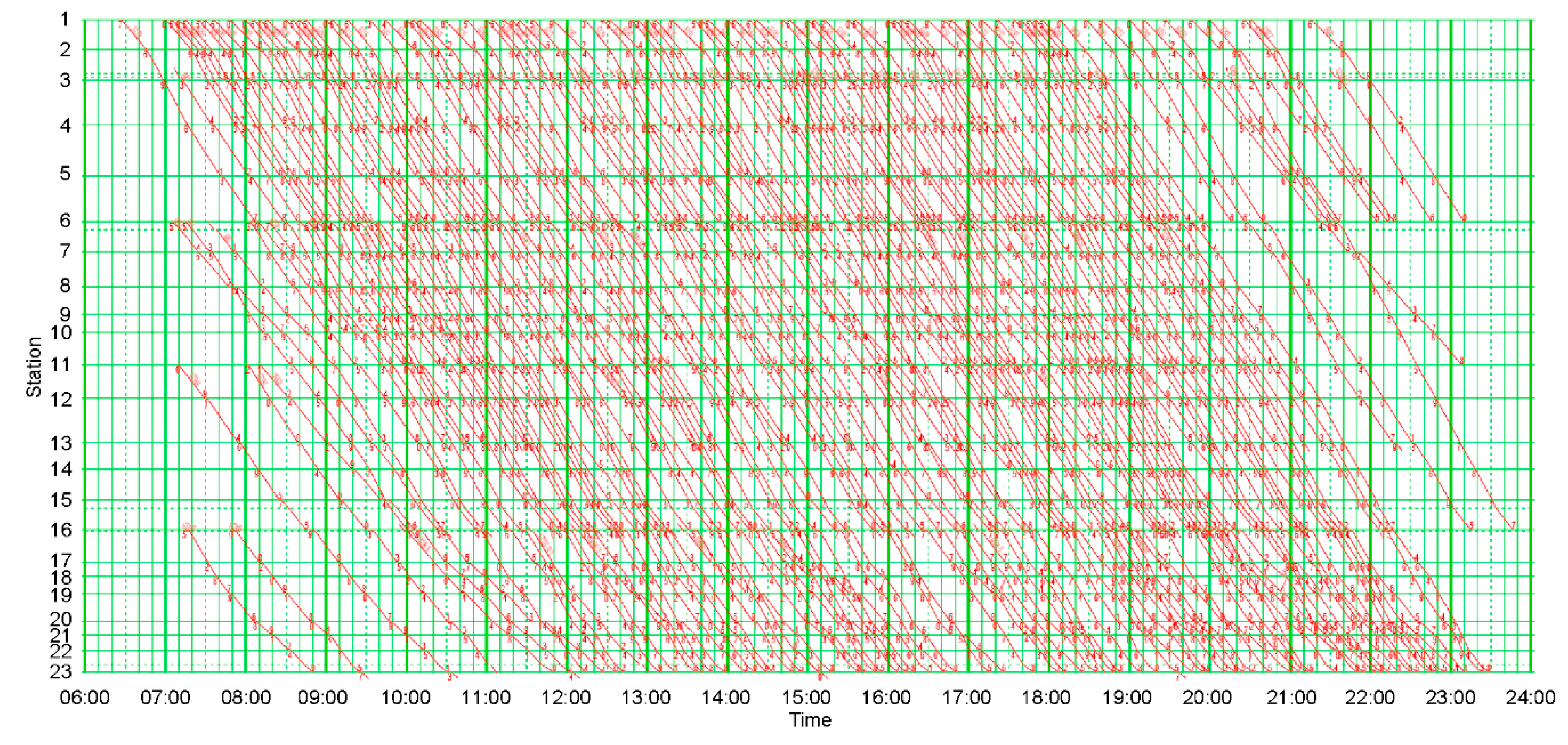
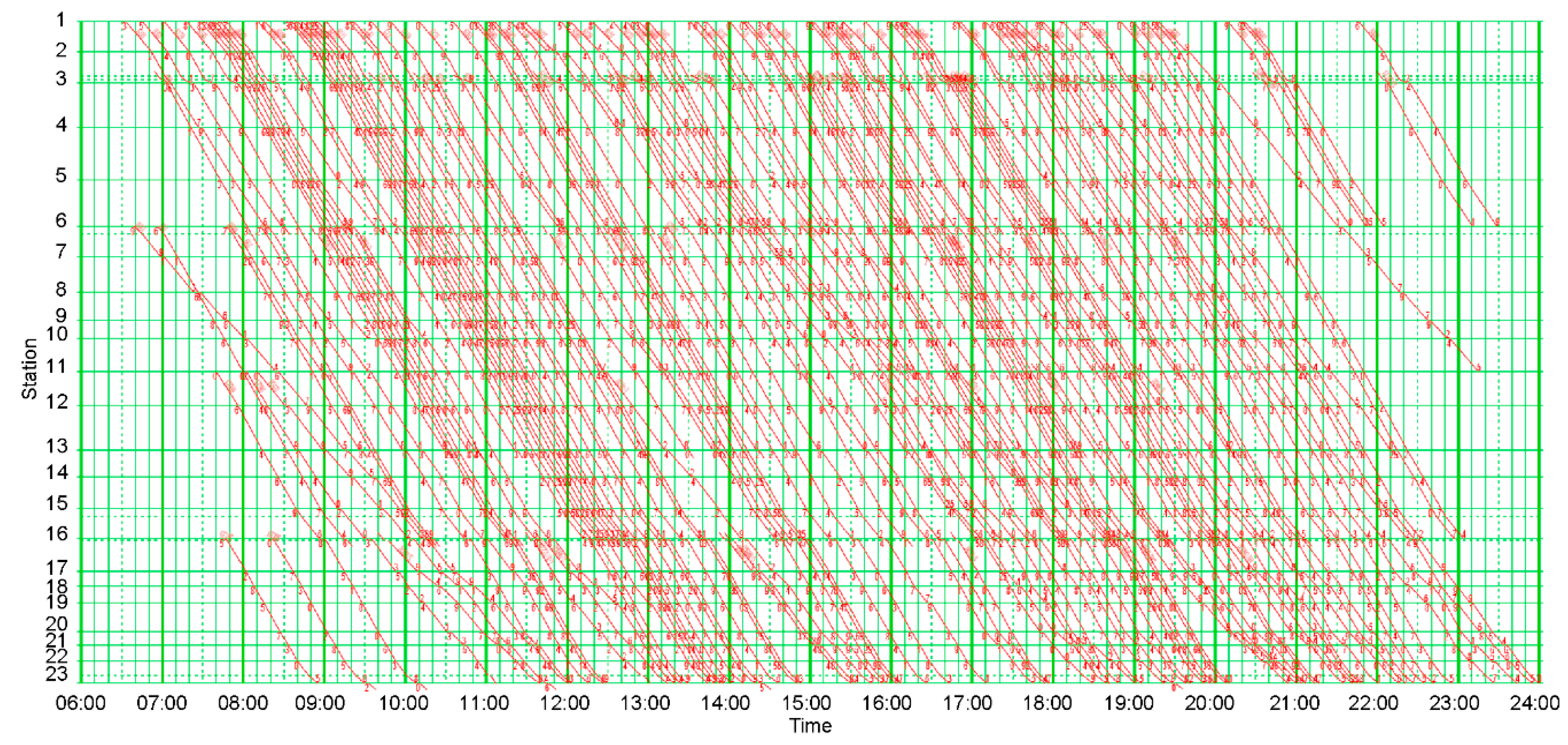
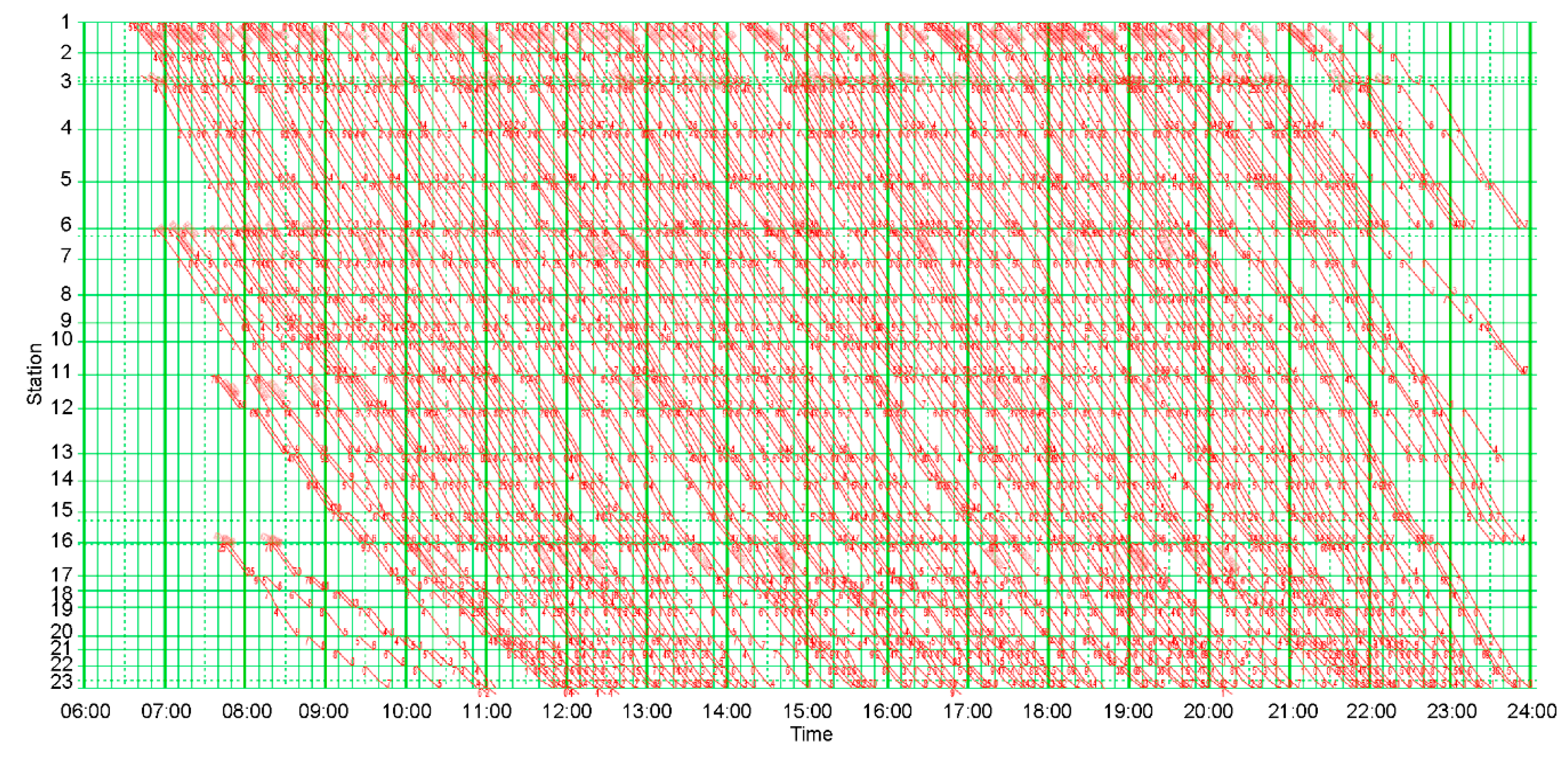
Figure 6 shows the actual train timetable for the Beijing–Shanghai HSR in May 2016, Figure 7 shows the optimal train timetable for Instance 3, and Figure 8 shows the optimal train timetable for Instance 5. The number of train stops and the stopping times of trains in Figure 7 are significantly reduced compared with those in Figure 6. More train trajectories are added to the train timetable in Figure 8 than in Figure 6 and Figure 7.
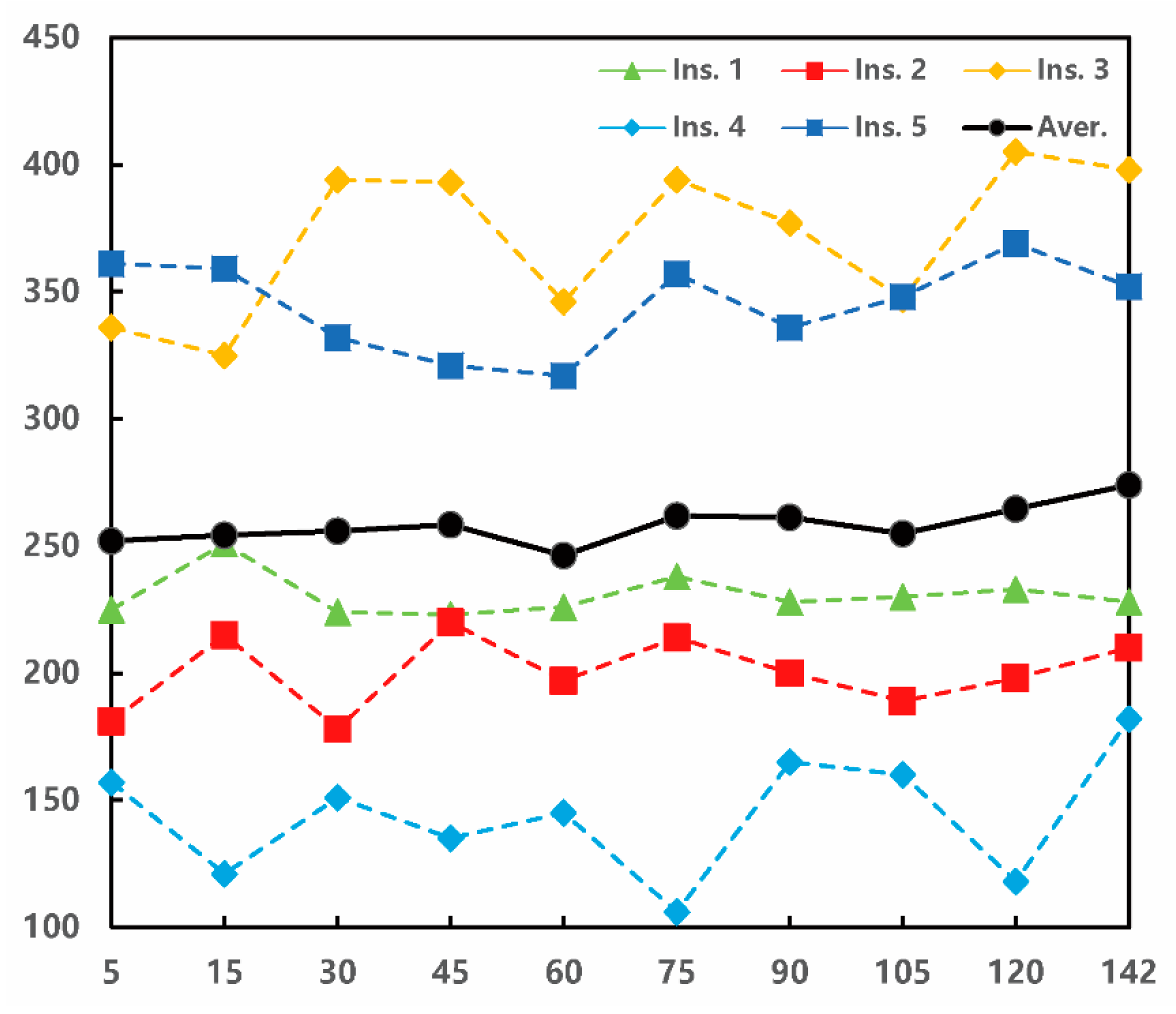
Figure 9 shows the experimental results of the optimal strategy tested in Case 5. The horizontal coordinates represent m in the partial pricing strategy and are valued as 5, 15, 30, 45, 60, 75, 90, 105, 120 and 142 (the number of all trains), and the vertical coordinates represent the time that it takes for the algorithm to reach the optimal value. Figure 9 shows that the differences in m have a great impact on the performance of the algorithm. Generally, when m = 60 , the computing speed of the algorithm is the fastest because the number of sub-problems needed to be calculated in each iteration is small, and frequent iterations can effectively avoid the problem in which the paths generated by the same dual variables tend to cover the same arcs. The black solid line (representing the average computing time) shows that the partial pricing strategy is effective for improving the efficiency of the algorithm.
The above experiments show that the acceleration strategies proposed in this paper can effectively improve the traditional column generation-based algorithm.

6. Conclusions

In this paper, a space-time network method is used to study the optimization of an HSRTTP. To satisfy the passenger service demands and maximize the total number of trains, two 0–1 linear integer programming models are established. These models are solved with a column generation-based algorithm, but, in the process of solving, we find that the algorithm has the shortcomings of a slow convergence speed and difficulty in obtaining integer solutions, so the computational efficiency is very low. In view of the existing problems of the algorithm, several acceleration strategies are proposed for each stage of the algorithm, and actual railway data were applied for a comparative analysis. The experimental results show that the acceleration strategies proposed in this paper can improve the computational efficiency of the algorithm to a certain extent. The optimal acceleration strategy has the best effect and increases the computational efficiency by 11.8× compared with that of the original algorithm.
In the future, our research will focus on three directions. First, only constraints concerning the limited number of sidetracks at a station were considered when optimizing the train timetable; constraints related to routing schedules and track use at stations will be considered [30]. Second, the passenger demands considered in this pager were derived from the daily passenger flow; the optimization of the HSR train timetable under time-varying passenger flow will be considered. Third, railway operators adopt energy saving (as well as energy recovery) strategies to reduce energy requirements; the optimization of the HSR train timetable with passenger demand and energy consumption will be studied.

Author Contributions

Conceptualization, L.Z. and Y.Y.; Data curation, J.W.; Formal analysis, J.W.; Funding acquisition, L.Z. and Y.Y.; Investigation, J.W.; Methodology, J.W. and Y.Y.; Project administration, L.Z. and Y.Y.; Resources, L.Z. and Y.Y.; Software, J.W.; Supervision, L.Z. and Y.Y.; Validation, L.Z. and Y.Y.; Visualization, J.W.; Writing—original draft, J.W.; and Writing—review and editing, J.W., L.Z., and Y.Y.

Funding

This research was funded by National Key R&D Program of China (2018YFB1201402) and the High-speed Rail Joint Fund of National Natural Science Foundation of China (U1834211).

Acknowledgments

The authors would like to thank the editors and the anonymous referees for their careful review and valuable suggestions that improved the quality of this paper.

Conflicts of Interest

The authors declare no conflict of interest.

References

  1. Dulebenets, M.A. A comprehensive multi-objective optimization model for the vessel scheduling problem in liner shipping. Int. J. Prod. Econ. 2018, 196, 293–318. [Google Scholar] [CrossRef]
  2. Jalalian, M.; Gholami, S.; Ramezanian, R. Analyzing the trade-off between CO2 emissions and passenger service level in the airline industry: Mathematical modeling and constructive heuristic. J. Clean. Prod. 2019, 206, 251–266. [Google Scholar] [CrossRef]
  3. Liu, L.; Chen, R.C. A novel passenger flow prediction model using deep learning methods. Trans. Res. Part C Emerg. Technol. 2017, 84, 74–91. [Google Scholar] [CrossRef]
  4. Wagenaar, J.; Kroon, L.; Fragkos, I. Rolling stock rescheduling in passenger railway transportation using dead-heading trips and adjusted passenger demand. Trans. Res. Part B Methodol. 2017, 101, 140–161. [Google Scholar] [CrossRef]
  5. Han, P.; Nie, L.; Fu, H.; Gong, Y.; Wang, G. A Multiobjective Integer Linear Programming Model for the Cross-Track Line Planning Problem in the Chinese High-Speed Railway Network. Symmetry 2019, 11, 670. [Google Scholar] [CrossRef]
  6. Liu, S.; Lin, B.; Wu, J.; Zhao, Y. Modeling the service network design problem in railway express shipment delivery. Symmetry 2018, 10, 391. [Google Scholar] [CrossRef]
  7. Qu, Z.; He, S. A Time-Space Network Model Based on a Train Diagram for Predicting and Controlling the Traffic Congestion in a Station Caused by an Emergency. Symmetry 2019, 11, 780. [Google Scholar] [CrossRef]
  8. Niu, H.; Zhou, X.; Gao, R. Train scheduling for minimizing passenger waiting time with time-dependent demand and skip-stop patterns: Nonlinear integer programming models with linear constraints. Trans. Res. Part B Methodol. 2015, 76, 117–135. [Google Scholar] [CrossRef]
  9. Yue, Y.; Wang, S.; Zhou, L.; Tong, L.; Saat, M.R. Optimizing train stopping patterns and schedules for high-speed passenger rail corridors. Trans. Res. Part C Emerg. Technol. 2016, 63, 126–146. [Google Scholar] [CrossRef]
  10. Zhou, L.; Tong, L.C.; Chen, J.; Tang, J.; Zhou, X. Joint optimization of high-speed train timetables and speed profiles: A unified modeling approach using space-time-speed grid networks. Trans. Res. Part B Methodol. 2017, 97, 157–181. [Google Scholar] [CrossRef] [Green Version]
  11. Jiang, F.; Cacchiani, V.; Toth, P. Train timetabling by skip-stop planning in highly congested lines. Trans. Res. Part B Methodol. 2017, 104, 149–174. [Google Scholar] [CrossRef]
  12. Adenso-Dıaz, B.; González, M.O.; González-Torre, P. On-line timetable re-scheduling in regional train services. Trans. Res. Part B Methodol. 1999, 33, 387–398. [Google Scholar] [CrossRef]
  13. Kroon, L.G.; Dekker, R.; Vromans, M.J. Cyclic railway timetabling: A stochastic optimization approach. In Algorithmic Methods for Railway Optimization; Springer: Berlin, Germany, 2007; pp. 41–66. [Google Scholar] [CrossRef]
  14. Zhou, L.; Hu, S.; Ma, J.; Yue, Y. Network Hierarchy Parallel Algorithm of Automatic Train Scheduling. J. China Railw. Soci. 1998, 20, 15–21. [Google Scholar]
  15. Shi, F.; Wei, T.; Zhou, W.; Luo, X. Optimization method for train diagram of high-speed railway considering the turnover of multiple units and the utilization of arrival-departure tracks. China Railw. Sci. 2012, 33, 107–114. [Google Scholar] [CrossRef]
  16. Caprara, A.; Monaci, M.; Toth, P.; Guida, P.L. A Lagrangian heuristic algorithm for a real-world train timetabling problem. Discret. Appl. Math. 2006, 154, 738–753. [Google Scholar] [CrossRef]
  17. He, B.; Song, R.; He, S.; Xu, Y. High-speed rail train timetabling problem: A time-space network based method with an improved branch-and-price algorithm. Math. Problems Eng. 2014, 2014. [Google Scholar] [CrossRef]
  18. Lu, C.; Zhou, L.; Chen, R. Optimization of high-speed railway timetabling based on maximum utilization of railway capacity. J. Railw. Sci. Eng. 2018, 15, 32–40. [Google Scholar] [CrossRef]
  19. Wang, J.; Zhou, L.; Yue, Y.; Tang, J.; Bai, Z. Optimizing High-Speed Railroad Timetable with Passenger and Station Service Demands: A Case Study in the Wuhan-Guangzhou Corridor. J. Adv. Trans. 2018, 2018. [Google Scholar] [CrossRef]
  20. Chen, S.; Shen, Y. Accelerating Column Generation for Solving Crew Scheduling Problems. J. Trans. Syst. Eng. Inf. Technol. 2014, 14, 144–149. [Google Scholar] [CrossRef]
  21. Desaulniers, G.; Desrosiers, J.; Solomon, M.M. Accelerating strategies in column generation methods for vehicle routing and crew scheduling problems. In Essays and Surveys in Metaheuristics; Springer: New York, NY, USA, 2002; pp. 309–324. [Google Scholar] [CrossRef]
  22. Gamache, M.; Soumis, F.; Marquis, G.; Desrosiers, J. A column generation approach for large-scale aircrew rostering problems. Oper. Res. 1999, 47, 247–263. [Google Scholar] [CrossRef]
  23. Ryan, D.; Foster, B. An Integer Programming Approach to Scheduling. Comput. Sched. Public Trans. 1981, 82, 269–280. [Google Scholar]
  24. Danna, E.; Pape, C. Branch-and-price heuristics: A case study on the vehicle routing problem with time windows. In Column Generation; Springer: Boston, MA, USA, 2005; pp. 99–129. [Google Scholar] [CrossRef]
  25. Savelsbergh, M. A branch-and-price algorithm for the generalized assignment problem. Oper. Res. 1997, 45, 831–841. [Google Scholar] [CrossRef]
  26. Sigurd, M.M.; Ulstein, N.L.; Nygreen, B.; Ryan, D.M. Ship scheduling with recurring visits and visit separation requirements. In Column Generation; Springer: Boston, MA, USA, 2005; pp. 225–245. [Google Scholar] [CrossRef]
  27. Sol, M.; Savelsbergh, M.W.P. A Branch-and-Price Algorithm for the Pickup and Delivery Problem with Time Windows; Eindhoven University of Technology, Department of Mathematics and Computing Science: Lyngby, Denmark, 1994. [Google Scholar]
  28. Zhou, X.; Zhong, M. Bicriteria train scheduling for high-speed passenger railroad planning applications. Eur. J. Oper. Res. 2005, 167, 752–771. [Google Scholar] [CrossRef]
  29. Goffin, J.L.; Vial, J.P. Multiple cuts in the analytic center cutting plane method. SIAM J. Optim. 2000, 11, 266–288. [Google Scholar] [CrossRef]
  30. Zhang, Q.; Zhu, X.; Wang, L. Track Allocation Optimization in Multi-Direction High-Speed Railway Stations. Symmetry 2019, 11, 459. [Google Scholar] [CrossRef]
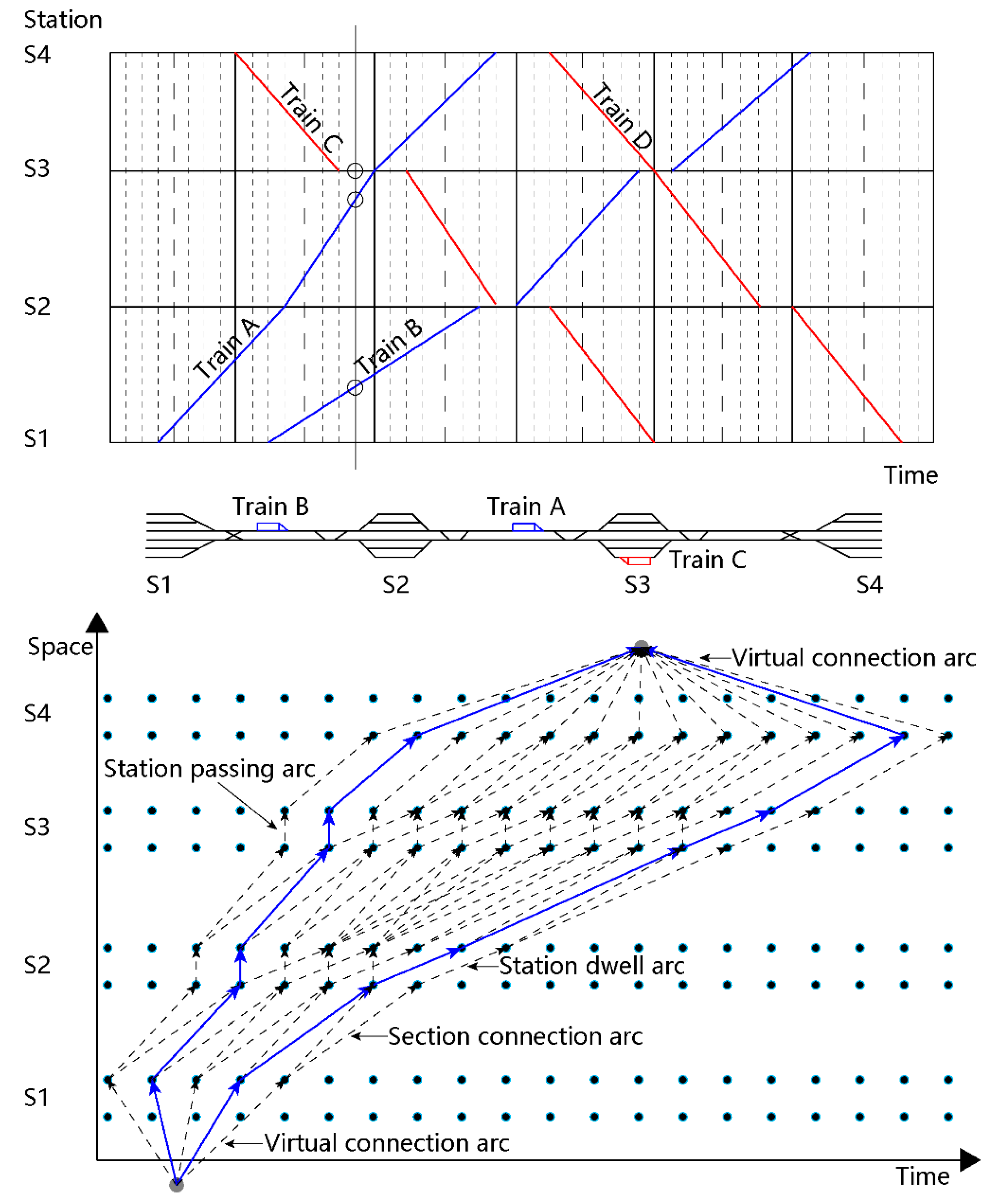
Figure 1. Relationships among the train timetable, railway lines and space-time network. The upper part of Figure 1 represents a train timetable, the middle part represents a railway line and the lower part represents a space-time network diagram.
Symmetry 11 00983 g001
Figure 2. Elimination of the redundant arcs.
Symmetry 11 00983 g002
Figure 3. Illustration of the delayed constraint strategy.
Symmetry 11 00983 g003
Figure 4. Diagram of the Beijing–Shanghai HSR.
Symmetry 11 00983 g004
Figure 5. Variation in the objective function value of the root node over time: (a) the objective function curve of Model M1; and (b) the objective function curve of Model M2.
Symmetry 11 00983 g005
Figure 6. The actual train timetable for the Beijing–Shanghai HSR.
Symmetry 11 00983 g006
Figure 7. The optimal train timetable for Instance 3.
Symmetry 11 00983 g007
Figure 8. The optimal train timetable for Instance 5.
Symmetry 11 00983 g008
Figure 9. Experimental results of the optimal strategy tested in Case 5.
Symmetry 11 00983 g009
Table 1. Notations.
Table 1. Notations.
SymbolDefinition
Subscripts
t Index of times, t T , where T is the set of time intervals, T = { 0 , 1 , , 1440 } ;
i , i Index of stations, i , i S : i i , where S is the set of stations;
j Index of trains, j N , where N is the set of trains, | N | = l ;
p , p Index of paths, p , p P : p p , where P is the set of paths;
e Index of sections, e E , where E is the set of sections;
Sets
P j Space-time path set belonging to train j ;
P e Space-time path set passing section e ;
Input parameters
c p 1 , c p 2 Cost of a space-time path for different mathematical models;
t p , e dep , t p , e arr Time when a train enters and leaves section e ;
t e dep , t e arr Minimum departure headway and minimum arrival headway of section e ;
t p , i beg , t p , i end Arrival time and departure time of station i in path p ;
t i min , t i max Minimum and maximum dwell time requirements for station i ;
n i Number of side tracks at station i ;
μ p i Stop index, which is equal to 1 if path p stops at station i and is equal to 0 otherwise;
τ p i , i Coupled-stop index, which is equal to 1 if path p stops at both station i and station i and is equal to 0 otherwise, τ p i , i = μ p i μ p i ;
β 1 Penalty coefficient of the number of train stops, the unit is 1/num;
β 2 Penalty coefficient of the stopping time, the unit is 1/min;
v i , i Minimum number of direct trains serving the passenger flow from station i to station i ;
Q i , i Average passenger flow OD matrix from station i to station i over a period of time counted by the passenger ticket department, the unit is one person;
φ Passenger capacity of a train, the unit is one person;
w i , i Average attendance rate of the trains from station i to station i .
Table 2. Overview of the Beijing–Shanghai HSR.
Station NameStation IDDistance (km)Number of Tracks
Downward DirectionUpward DirectionAll
Beijing South10202024
Langfang2596612
Tianjin South3131446
Cangzhou West4219668
Dezhou East53278812
Jinan West6419101117
Taian7462668
Qufu East8533668
Tengzhou East9589334
Zaozhuang10625668
Xuzhou East1168891015
Suzhou East12767668
Bengbu South13844101114
Dingyuan14897334
Chuzhou15959446
Nanjing South1610186610
Zhenjiang South171087668
Danyang North181112334
Changzhou North191144668
Wuxi East201201668
Suzhou North211227668
Kunshan South221259446
Shanghai Hongqiao231302101119
Table 3. Section travel time of the Beijing–Shanghai HSR.
Adjacent Station PairSection Travel Time (min)
Grade GGrade D
1–21922
2–31316
3–41822
4–52226
5–62023
6–71315
7–81518
8–91214
9–1089
10–111416
11–121417
12–131822
13–141214
14–151316
15–161619
16–171720
17–1867
18–1978
19–201214
20–2167
21–2278
22–231517
Table 4. OD service frequency data for the downward direction.
Station1234567891011121314151617181920212223
181188148888118112814958810814
2522822225251281222428
355115555838041112537311
42822225252283222428
5822225252283122428
68888118113814978810814
72225251283122428
8225250283222428
925252283222428
105251283222428
1158551165557511
1252283222428
13351165557511
14262222425
1583222428
16988810814
17333539
1822428
192428
20428
21410
228
23
Table 5. Comparisons of the results for different train timetables.
ParametersActual CaseM1M2
Number of trains142142200
Average travel speed (km/h)216.1238.2213.2
Average number of stops5.22.85.2
Average dwell time (min)16.26.815.8
Overtaking12438281
Max dwell time of Grade G (min)12712
Max dwell time of Grade D (min)342528
Table 6. Five instances designed for the Beijing–Shanghai HSR.
StationInstanceStationInstance
1234512345
1NNNNN13NYYNY
2NYYNY14YNYNY
3NYYNY15NYYNY
4NYYNY16YNYNY
5YNYNY17NYYNY
6NYYNY18NYYNY
7NYYNY19NYYNY
8YNYNY20NYYNY
9NYYNY21NYYNY
10NYYNY22NYYNY
11NYYNY23NNNNN
12NYYNY
Table 7. Comparisons of different cases.
InstanceCase 1Case 2Case 3Case 4Case 5
TimeGapTimeGapTimeGapTimeGapTimeGap
125640.30218470.28212150.2877800.1252230.109
224410.6321870.52210150.52223010.5151780.162
340190.6119450.60021640.60013640.1843250.154
420280.45513270.4559070.4605440.3451060.363
525750.46323190.46315200.4708670.3253170.288
Average27250.49219250.46413640.46811710.2992300.215