Design and Experiment of Symmetrical Shape Deployable Arc Profiling Mechanism Based on Composite Multi-Cam Structure

Abstract

At present, there are few reports on the profiling mechanism that can achieve surface envelope profiling along the surface of a shaft whose radius is constantly changing. Existing profiling mechanisms cannot achieve this function. To this end, a novel deployable arc profiling mechanism is presented in this paper. The mechanism can realize centering deployment along the shaft with a changing radius. The radius of the deployable arc can be adapted to the continuous change of shaft radius, and its surface can always maintain the arc shape for surface envelope profiling. The mechanism is mainly composed of compound cams. Each cam contains multiple grooves, and each groove connects to an arc support linkage. The arc support linkage is controlled by the compound motion of cams in different layers. The pitch curve of each groove is designed by applying the method of relative motion and inverse solution and obtained various parameter equations of the mechanism. The feasibility of this mechanism is verified by analysis, experiment, and application test. The results show that the proposed deployable arc profiling mechanism can achieve the design purpose and the profiling accuracy is kept above 96.425%.

1. Introduction

Profiling process is based on a pre-made model, which enables a cutting tool to perform synchronously copying action by using a profiling mechanism, so that the parts with the same profile can be machined on the part blank [1]. Profiling process has the characteristics of requiring profiling mechanism and pre-made model, it uses a profiling mechanism to carry out passive copying processing [2]. With the development of CNC machine technology, the profiling mechanism is no longer necessary, but precise measurement, sensor, and control system are needed [3]. The profiling mechanism is basically replaced by these electronic systems, which reduces the dependence on the profiling mechanism and also reduces research on it. However, the structure of early profiling mechanism is relatively simple, and most of them are profiled along a fixed path or curved surface of the convex plate. As a result, there are few reports about the profiling mechanism that can achieve surface envelope profiling along the surface of a shaft whose radius is constantly changing.

The surface envelope profiling along a radius-changing shaft can be understood as the arc of the shaft surface runs a deploying movement within the radius of the shaft. At the same time, the profiling parts of the profiling mechanism to be designed also carry out the synchronized envelope deploy motion along with the shaft. This kind of profiling mechanism has never been reported before, but the deployable mechanism which can carry out the movement can provide reference for designing it. As a new type of structure, the deployable mechanism has gradually attracted the attention of scholars and become a research hotspot [4]. In 1960, Buckminster Fuller, an American architect, first proposed the concept of deployable structure. Subsequently, E. P. Pineo [5] successfully applied the concept to design the deployable dome structure of movable theatre. In this deployable dome structure, when it is deployed, a fixed shape of an arc can be formed on it. NASA has developed a large number of deployable space antenna systems, that when it is deployed, a fixed shape of the curved surface can be formed [6,7,8]. Deployable mechanism with polyhedron shape different from an arc or a curved surface was also proposed [9]. With the introduction of flexible components, a rigid-flexible coupling state was appeared in the deployable mechanism [10]. The related design methods such as graph theory, flow value method, bionics method, and topology method were also reported [11,12,13,14]. The reports of these deployable mechanisms emphasized the final shape that can be maintained after deployed, but the dynamically changing shape that can be maintained in the process of deploying was not the focus of research. Nevertheless, previous reports can provide useful references for the design of the deployable arc profiling mechanism which can maintain the arc shape during the deployment in this paper.

In order to achieve complex motion, some deployable mechanisms were driven by the cam mechanism. Cam mechanism has the advantages of high motion precision, easy driving, compact structure, and convenient design, and has been widely used. Giorgio Figliolini [15] proposed a composite cam mechanism with curved grooves. Jyh-Jone Lee [16,17,18] eliminated the impact load at the beginning and the end of the motion. Ion Simionescu [19,20,21] designed the self-centering statically determinate grippers, has two and three fingers, used to handle the work piece with a cylindrical shape. The related mathematical models of the self-centering grippers are obtained, and the optimum synthesis of the two fingers self-centering grippers are also showed. Chen Junhua [22] solved the problem of errors in the design of cam plane contour. Ren-Chung Soong [23,24] designed a cam transmission mechanism for generating precise trajectories. Nelson, Todd G. [25] designed the structure of the deployable cam and achieved the transition of a rolling element from a plane state to a deployed state. Changjiang Zhou [26] reduced the vibration of the cam mechanism. Li Meng [27] satisfies the specific dynamic requirements of the deployable mechanism by using a cam mechanism. These studies have gradually improved the motion accuracy and reliability of the cam mechanism, and also applied it to the deployable mechanism. It provided the basic theories and references for the design of the composite multi-cam structure.

In this paper, by analyzing the dynamic change process of deployable arc in deploying motion, the motion trajectory of compound cams that drives the deployable arc is obtained. Then make the obtained motion trajectory motion-decomposed, after it, the parametric equation of the pitch curve of each cam groove is obtained. Finally, a symmetrical shape of deployable arc profiling mechanism is designed out. The theoretical analysis, experimental verification, and practical application test (applied to the banana crown cutting device) of this mechanism are carried out. The results show that the mechanism can perform surface envelope profiling well along the shaft surface with the changing radius. The obtained parametric equations have practical application value.

2. Description of Deployable Arc Profiling Mechanism

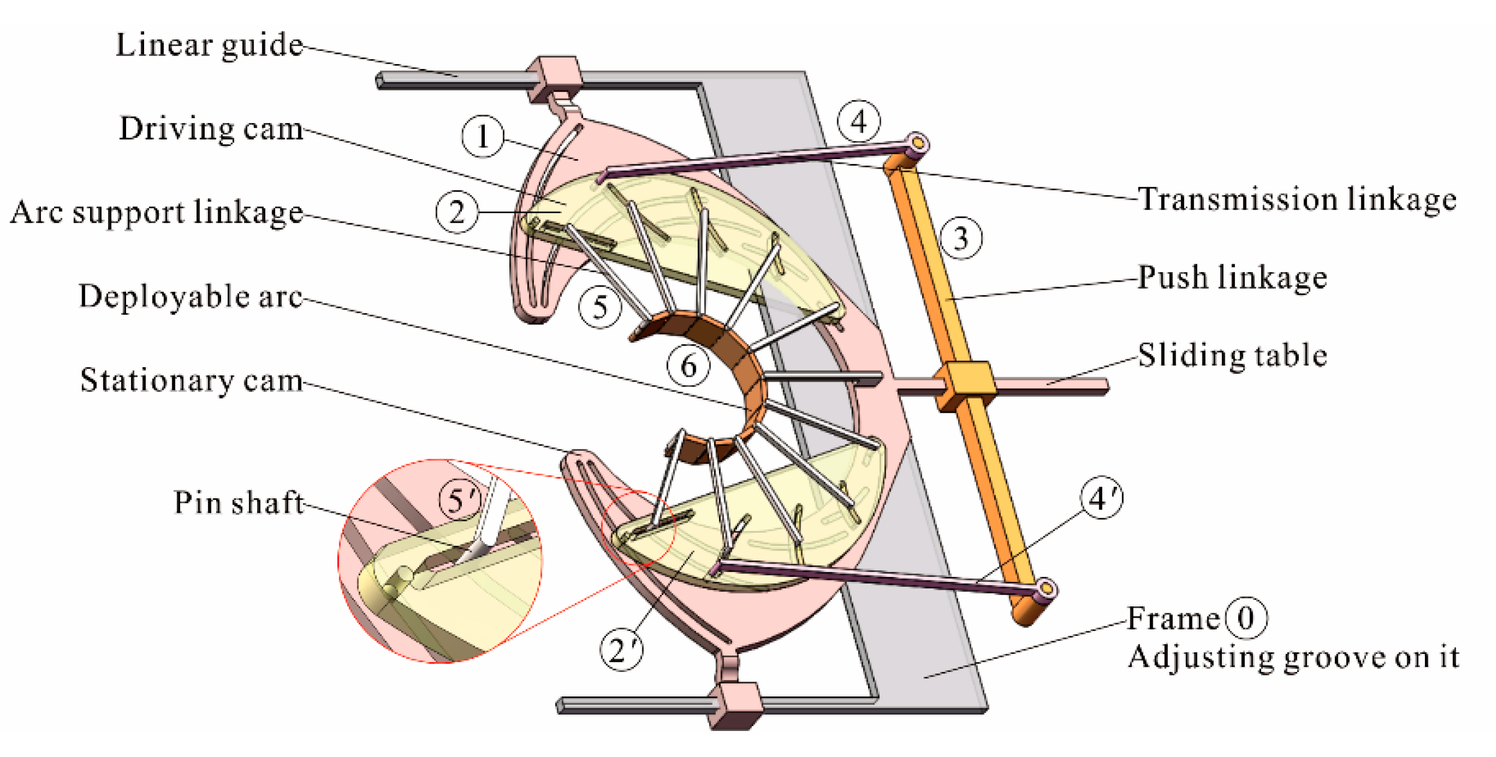
2.1. Structure of Mechanism

The deployable arc profiling mechanism presented in this paper is shown in Figure 1. The mechanism is made up of upper, middle, and lower three-layer plane. Multiple grooves are distributed in each cam. The upper layer consists of two driving cams, a deployable arc, and multiple arc support linkages. The middle layer consists of a stationary cam, a sliding table, a push linkage, and two transmission linkages. The lower layer consists of an adjusting groove and two linear guides. The lower layer is fixed on the machine frame. The middle layer is installed on the lower layer’s two linear guides. The upper layer is connected to the middle layer by using the push linkage and transmission linkages. One end of the transmission linkages is connected to the driving cams, and the other end is connected to the push linkage. The sliding table on the middle layer drives the push linkage to drive the mechanism. All the arc support linkages are connected to the deployable arc with hinges. The arc lengths between any two adjacent connection points are equal. The other end of the arc support linkages is connected to the two driving cams by using pin shaft. All the pin shafts are welded to its corresponding arc support linkages, and perpendicular to it. Among these pin shafts, there are two pin shafts symmetrically installed along the center line of mechanism and pass through three grooves of the upper, middle, and lower layers’ cams at the same time. The rest of the pin shafts only pass through two grooves of upper- and middle-layers’ cams. The mechanism is a plane motion pair composed of cam grooves. The deploying movement of the arc is driven by the interaction between the driving of push linkage and the relative motion of composite multi-cam. The final result of the movement is that the deployable arc can be deployed around a fixed arc center and achieve continuous change of the arc radius.

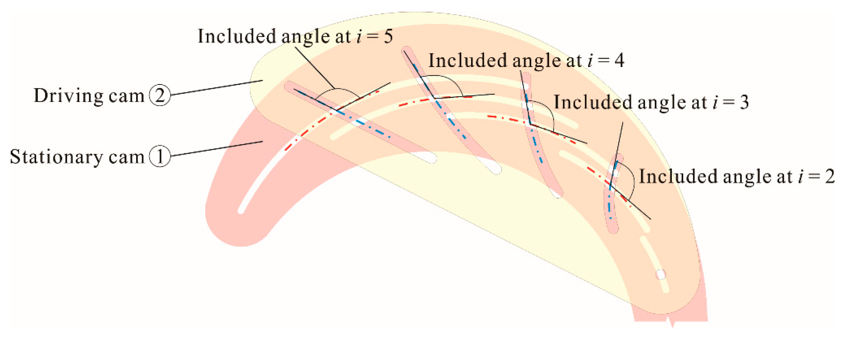
2.2. Design Principle of Mechanism

In the process of gradually deploying of the arc, the arc length between any two points on the arc remains unchanged. These two points can form their own special motion trajectories. The positions of selected points are different, and the trajectories formed are also different. In order to make the deployable arc maintain its arc shape in the process of deploying, we can select several points on the deployable arc as the driving points and drive the arc according to these formed motion trajectories. In this way, the continuous deployable motion of the arc can be achieved. Among all the selected driving points, there is one point at each end of the arc and one point at the midpoint of the arc. The arc length between any two adjacent points is equal, and each driving point is connected with an arc support linkage. The center lines of all the arc support linkages intersect at the center of the arc, then the angle of all the adjacent arc support linkages is equal. As the arc gradually deploying, the free end of the arc support linkages can form special motion trajectories on the same plane. Since the angle and arc length between any two adjacent support linkages are equal, these motion trajectories can be calculated. The motion trajectory can be regarded as the pitch curve of the cam groove, and the obtained mathematical model is the model of the pitch curve. In this paper, the straight line passing through the midpoint of the arc and the center of the arc is the symmetrical center line of the deployable arc mechanism, all parts on the mechanism move symmetrically along it. We numbered the arc support linkages as shown in Figure 2. Apart from the fixed No. 0 support linkage, there are No. n (n = 1, 2, . . .) support linkages in the upper part of the mechanism.

3. Parameter Design of Deployable Arc Profiling Mechanism

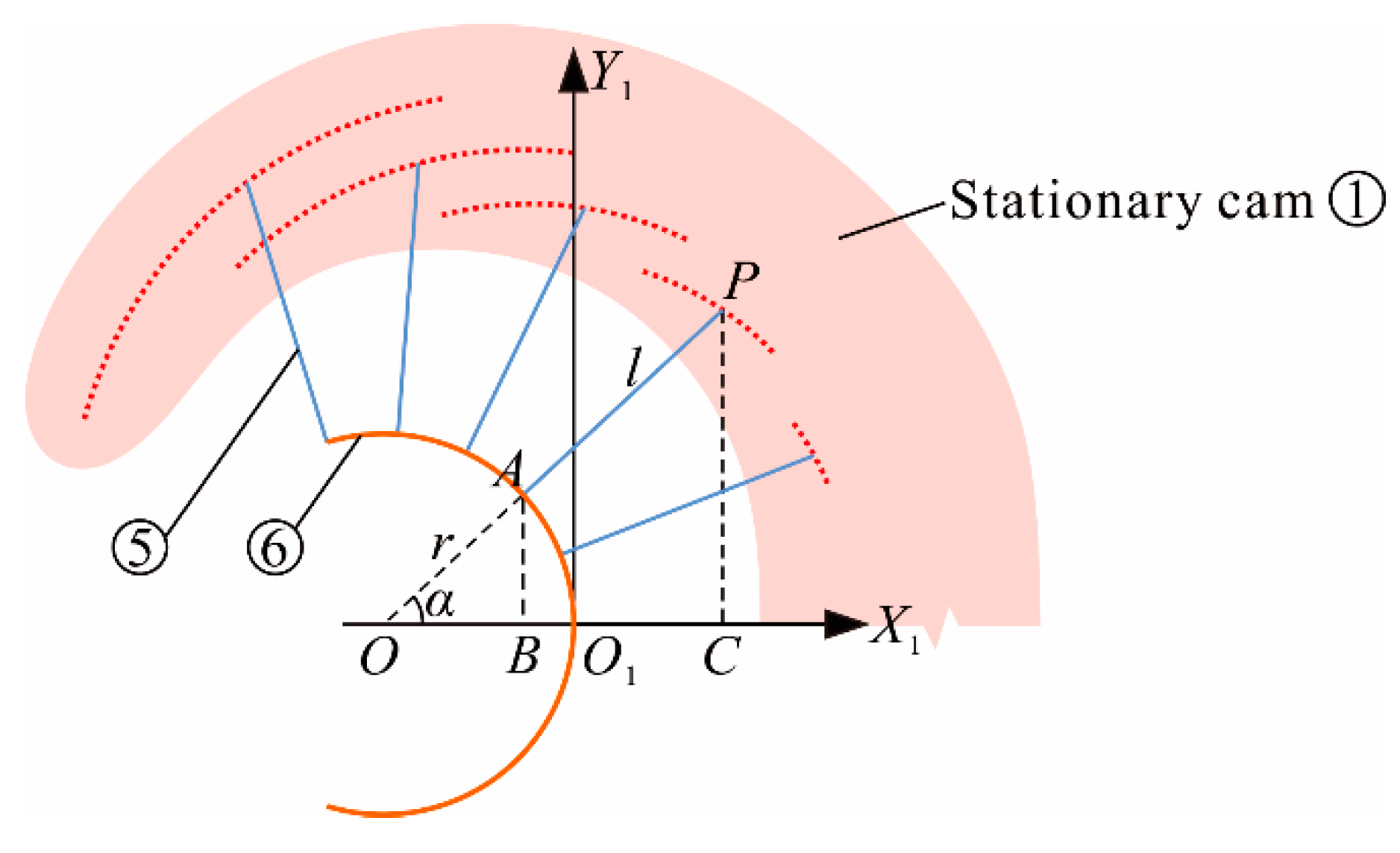
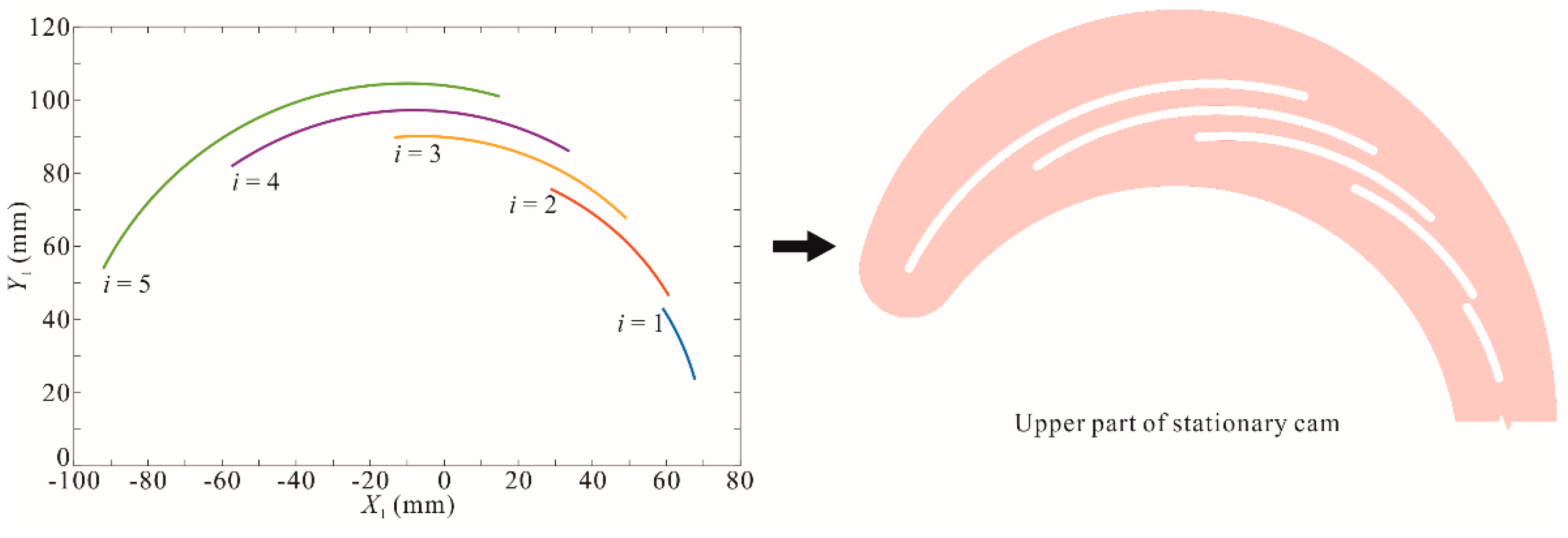
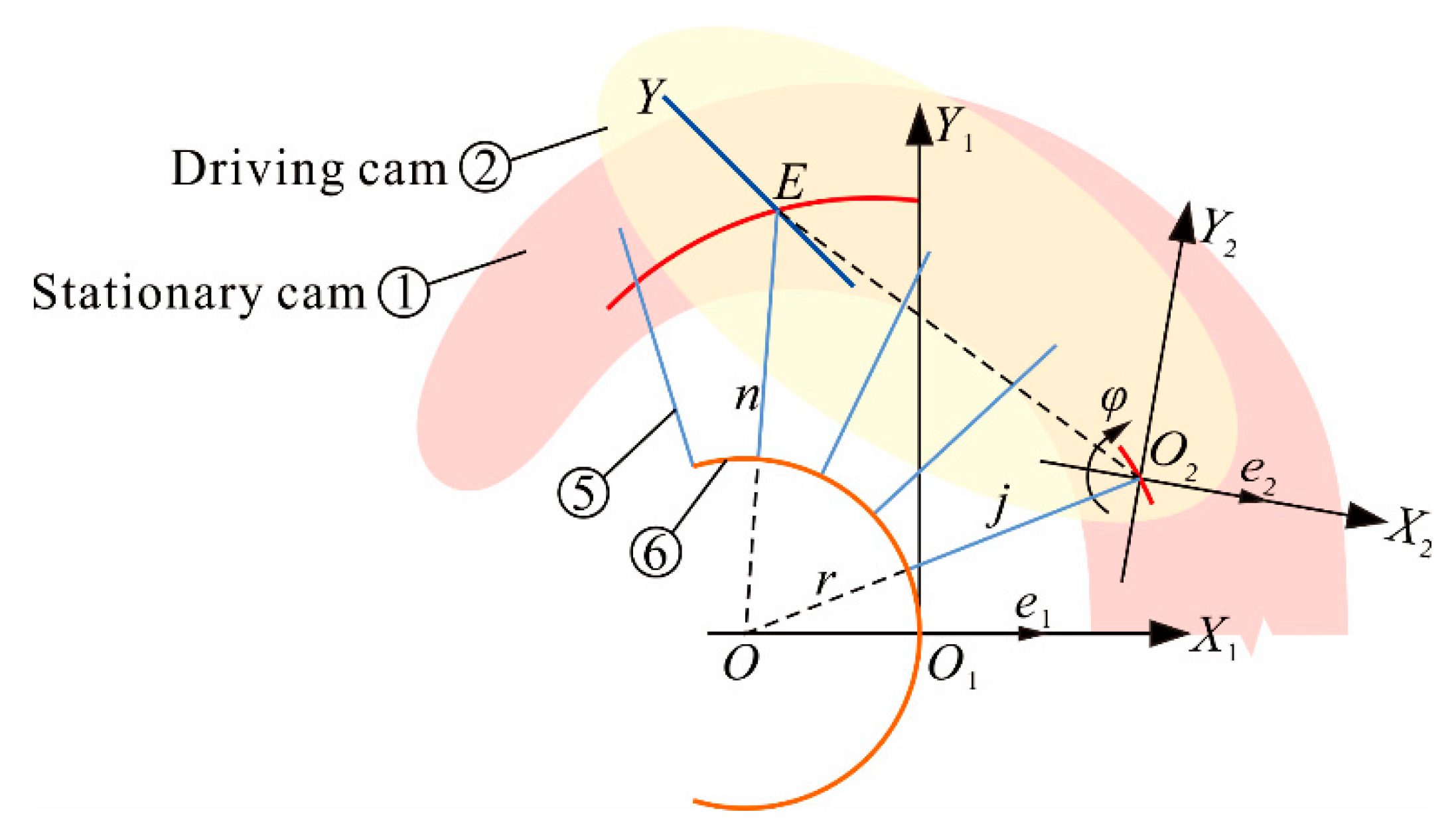
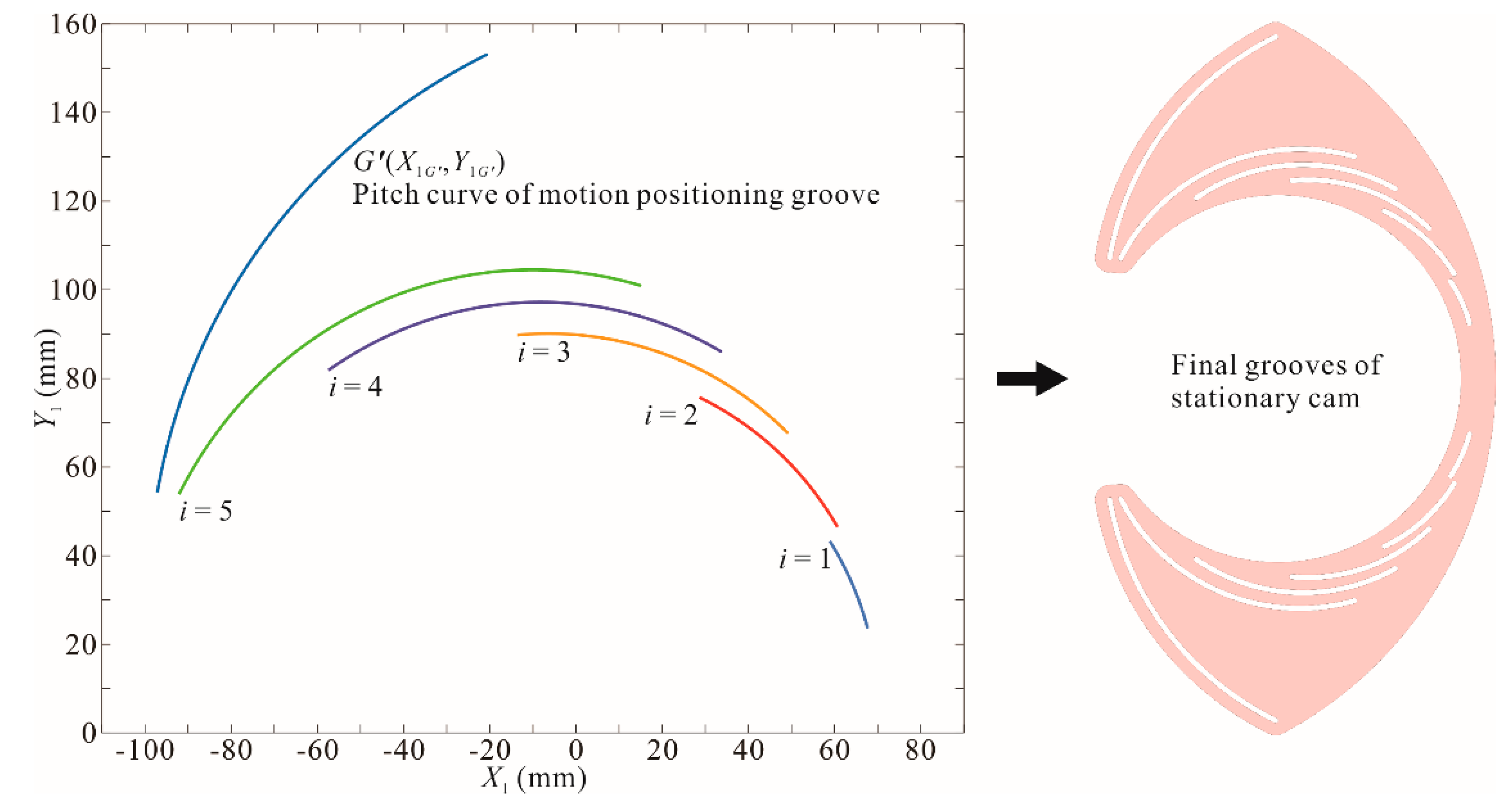
3.1. Pitch Curve of Stationary Cam Groove

The pitch curves of stationary cam grooves are the trajectories generated by the projection of the end of arc support linkages on stationary cam during the deploying process. The pitch curves are naturally formed in the process and are not affected by other cams. During designing the pitch curves of stationary cam grooves, take the midpoint of the deployable arc as the coordinate origin O₁, The No. i (i = 1, 2, . . ., i ≤ n) support linkage is connected to point A (X_1A, Y_1A) on the arc, and the end of this support linkage is point P (X_1P, Y_1P). The projections of points A and P on the X₁-axis are points B and C, respectively. The extension line of support linkage passes through the center of the arc at point O, as shown in Figure 3. The angle between extension line and X₁-axis is α, the radius of the arc is r, the length of arc support linkage is l, the arc length between any two adjacent support linkages is c.

With a change in the radius r of the arc, the angle α changes follow it, but the length of arc $\stackrel{⌢}{O_{1}A}$ remains unchanged. Since the arc length between any two adjacent support linkages is equal to c, the length of arc $\stackrel{⌢}{O_{1}A}$ is equal to ic, and the angle α = ic / r. Since point A is on the arc (X_1A + r)² + Y_1A² = r², (X_1A ≠ −2r), the coordinate of point A is (X_1A, $\sqrt{r^2-{(r+X_{1A})}^2}$). Owing to OA/OB = OP/OC and OA/AB = OP/PC, we can obtain equation:

$$\{\begin{array}{c}\frac{r}{r+X_{1A}}=\frac{r+l}{r+X_{1P}}\\ \frac{r}{\sqrt{r^2-{(r+X_{1A})}^2}}=\frac{r+l}{Y_{1P}}\end{array}$$

(1)

solving it we can get:

$$\{\begin{array}{c}{X}_{1P}=\frac{r+l}{r}(r+X_{1A})-r\\ Y_{1P}=\frac{r+l}{r}\sqrt{r^2-{(r+X_{1A})}^2}\end{array}$$

(2)

while cosα = (r + X_1A) / r and α = ic / r, so r + X_1A = rcos(ic / r). Take it into Equation (2), we can obtain the pitch curves of point P on stationary cam grooves as:

$$\{\begin{array}{c}{X}_{1P}=(r+l)\cos \frac{ic}{r}-r\\ Y_{1P}=(r+l)\sin \frac{ic}{r}\end{array}$$

(3)

where r is the radius of arc, l is the length of support linkage, and c is the arc length of segmented arc. If r varies from 20 to 50 mm, l = 70 mm, c = 10 mm, and the number of support linkages (in the upper part) is 5. The pitch curve at the end of No. i (i = 1~5) support linkage and the upper part of the stationary cam are shown in Figure 4.

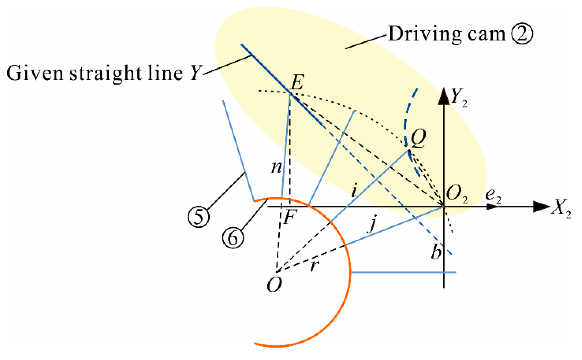
3.2. Parameter Design of Driving Cam

Parameter design of the driving cam consists of three parts:

• Pitch curve design of driving cam grooves, which can drive the support linkages to carry out regular movement.
• Driving motion equation design.
• Motion positioning groove design, which enables driving cam to be driven according to the resulted motion parameters.

3.2.1. Pitch Curve of Driving Cam Grooves

During the driving cam driving the arc support linkages, it performs a combined motion of translation and rotation. According to the principle of relative motion, the driving cam can be regarded as a fixed object, the support linkages driven by the driving cam is regarded as an active moving part. When the support linkages are moving, because the angle and the arc length between any two adjacent support linkages are equal. So, all the ends of support linkages exhibit a regular motion state during the movement, and their trajectories relative to driving cam can be found. These trajectories are the pitch curve of driving cam grooves.

In order to simplify the design process, we can make the motion trajectory of the end of any one support linkage is a given straight line Y = aX + b, and make the end of any other one support linkage as a fixed point, e.g., O₂ at the end of No. j (j = 1, 2, . . ., j ≠ n) support linkage shown in Figure 5. In this way, the motion trajectories of remaining support linkages can be obtained by the given straight line and the fixed point. This fixed point O₂ is taken as the coordinate origin, and the endpoint E of No. n support linkage is moving on the straight line. F is the projection point of point E on X₂-axis. The motion trajectory of point Q (X_2Q, Y_2Q) that located at the end of No. i support linkage is the pitch curve of driving cam groove.

Since point E is on the straight-line Y = aX + b, so the coordinate of point E on O₂-X₂Y₂ plane is (X_2E, aX_2E + b). Vector e₂ is a unit vector along X₂-axis on O₂-X₂Y₂ plane, so the angle between vector e₂ and vector O₂E is:

$$\langle \overrightarrow{e_2},\overrightarrow{O_{2}E}\rangle =\arccos \frac{X_{2E}}{\sqrt{X_{2E}{}^2+{(a{X}_{2E}+b)}^2}}$$

(4)

Since points E, Q, and O₂ are on the same arc, and point O is the center of the arc, then $\angle E{O}_{2}Q=\angle EOQ/2=(n-i)c/2r$. Since i ≤ n, $\angle E{O}_{2}Q$ is always positive. Therefore, the angle

$$\langle \overrightarrow{e_2},\overrightarrow{O_{2}Q}\rangle =\langle \overrightarrow{e_2},\overrightarrow{O_{2}E}\rangle -\angle E{O}_{2}Q=\arccos \frac{X_{2E}}{\sqrt{X_{2E}{}^2+{(a{X}_{2E}+b)}^2}}-\frac{(n-i)c}{2r}$$

(5)

In triangle OO₂Q, since the lengths of OO₂ and OQ are equal to r + l, and $\angle O_{2}OQ=(i-j)c/r$, we can obtain the length of O₂Q is:

$$\left|O_{2}Q\right|=2(r+l)\sin \frac{(i-j)c}{2r}$$

(6)

In the same way, the length of O₂E can be obtained as:

$$\left|O_{2}E\right|=2(r+l)\sin \frac{(n-j)c}{2r}$$

(7)

Then, the coordinate of point Q can be preliminarily determined as:

$$\{\begin{array}{c}{X}_{2Q}=\left|O_{2}Q\right|\cos \langle \overrightarrow{e_2},\overrightarrow{O_{2}Q}\rangle \\ Y_{2Q}=\left|O_{2}Q\right|\sin \langle \overrightarrow{e_2},\overrightarrow{O_{2}Q}\rangle \end{array}$$

(8)

Since the unknown variable X_2E exists, so the Equation (8) needs to be further solved.

There is an equation ${(a{X}_{2E}+b)}^2+X_{2E}{}^2={\left[2(r+l)\sin \frac{(n-j)c}{2r}\right]}^2$ in triangle O₂EF. Solve it can get:

$$X_{2E}=\frac{-ab-\sqrt{{(ab)}^2-(a^2+1)\left[b^2-4{(r+l)}^2\mathrm{s}\mathrm{i}{\mathrm{n}}^2\frac{(n-j)c}{2r}\right]}}{a^2+1}$$

(9)

Take Equation (9) into the coordinate of point Q. Finally, the parameter equation of pitch curve at the end of No. i support linkage on driving cam is obtained as:

$$\{\begin{array}{c}{X}_{2Q}=2(r+l)\sin \frac{(i-j)c}{2r}\cos \left[\arccos \frac{X_{2E}}{\sqrt{X_{2E}{}^2+{(a{X}_{2E}+b)}^2}}-\frac{(n-i)c}{2r}\right]\\ Y_{2Q}=2(r+l)\sin \frac{(i-j)c}{2r}\sin \left[\arccos \frac{X_{2E}}{\sqrt{X_{2E}{}^2+{(a{X}_{2E}+b)}^2}}-\frac{(n-i)c}{2r}\right]\end{array}$$

(10)

If r varies from 20 to 50 mm, l = 70 mm, c = 10 mm, j = 1, n = 5, and the straight line is Y = −X / 2. The pitch curve at the end of No. i support linkage and the upper part of driving cam are shown in Figure 6.

3.2.2. Driving Motion Equation

This section will present the motion equations of the driving cam, i.e., the translational trajectory of point O₂ and rotational motion around point O₂ on O₁-X₁Y₁ plane, as shown in Figure 5. The trajectory of point O₂ and point E on O₂-X₂Y₂ plane can be expressed by Equation (3), then, i = j corresponds to point O₂, and i = n corresponds to point E in Equation (3). Thus, the translational trajectory equation of point O₂ (base point) on O₁-X₁Y₁ plane is:

$$\{\begin{array}{c}{X}_{1O_2}=(r+l)\cos \frac{jc}{r}-r\\ Y_{1O_2}=(r+l)\sin \frac{jc}{r}\end{array}$$

(11)

Similarly, the translational trajectory equation of point E on O₁-X₁Y₁ plane is:

$$\{\begin{array}{c}{X}_{1E}=(r+l)\cos \frac{nc}{r}-r\\ Y_{1E}=(r+l)\sin \frac{nc}{r}\end{array}$$

(12)

In order to obtain the rotational motion equation of driving cam, a coordinate system is established, as shown in Figure 7. Point E is an intersection point between the introduced straight line on driving cam and the No. n groove on stationary cam. e₁ is a unit vector along X₁-axis direction on O₁-X₁Y₁ plane, and e₂ is a unit vector along X₂-axis direction on O₂-X₂Y₂ plane. Vector e₁ is fixed on the symmetrical center line of the mechanism, and vector e₂ is moved relative to vector e₁ on the driving cam. φ is the angle between vector e₂ and vector e₁. When e₂ is parallel to e₁ and in the same direction, the value of angle φ is zero. When e₂ moves counterclockwise with respect to e₁ and through the zero position, the value of φ is a positive number, while when it is clockwise with respect to e₁ and through the zero position, the value of φ is a negative number. The direction of rotation of φ marked in Figure 7 is the direction of the deployable arc in deploying motion, and φ is a negative value at this time. The rotational motion equation of driving cam relative to stationary cam is a rotation vector of vector e₂ relative to vector e₁. The rotation angle φ of driving cam can be obtained according to the change of rotation vector of vector O₂E that is relative to vectors e₁ and e₂.

On O₁-X₁Y₁ plane, vector O₂E can be derived by the parameter equations of points O₂ and E, the angle between vectors e₁ and O₂E can be calculated. So, the rotation vector O₂E relative to e₁ on O₁-X₁Y₁ plane is:

$$\langle \overrightarrow{e_1},\overrightarrow{O_{2}E}\rangle =\pi -\arccos \left[\sin \frac{(n+j)c}{2r}\right]$$

(13)

According to Equation (4), vector O₂E = (X_2E, aX_2E + b), and rotational change of vector O₂E relative to vector e₂. The rotation angle φ on driving cam can finally obtained as:

$$\phi =\pi -\arccos \left[\sin \frac{(n+j)c}{2r}\right]-\arccos \frac{X_{2E}}{\sqrt{X_{2E}{}^2+{(a{X}_{2E}+b)}^2}}$$

(14)

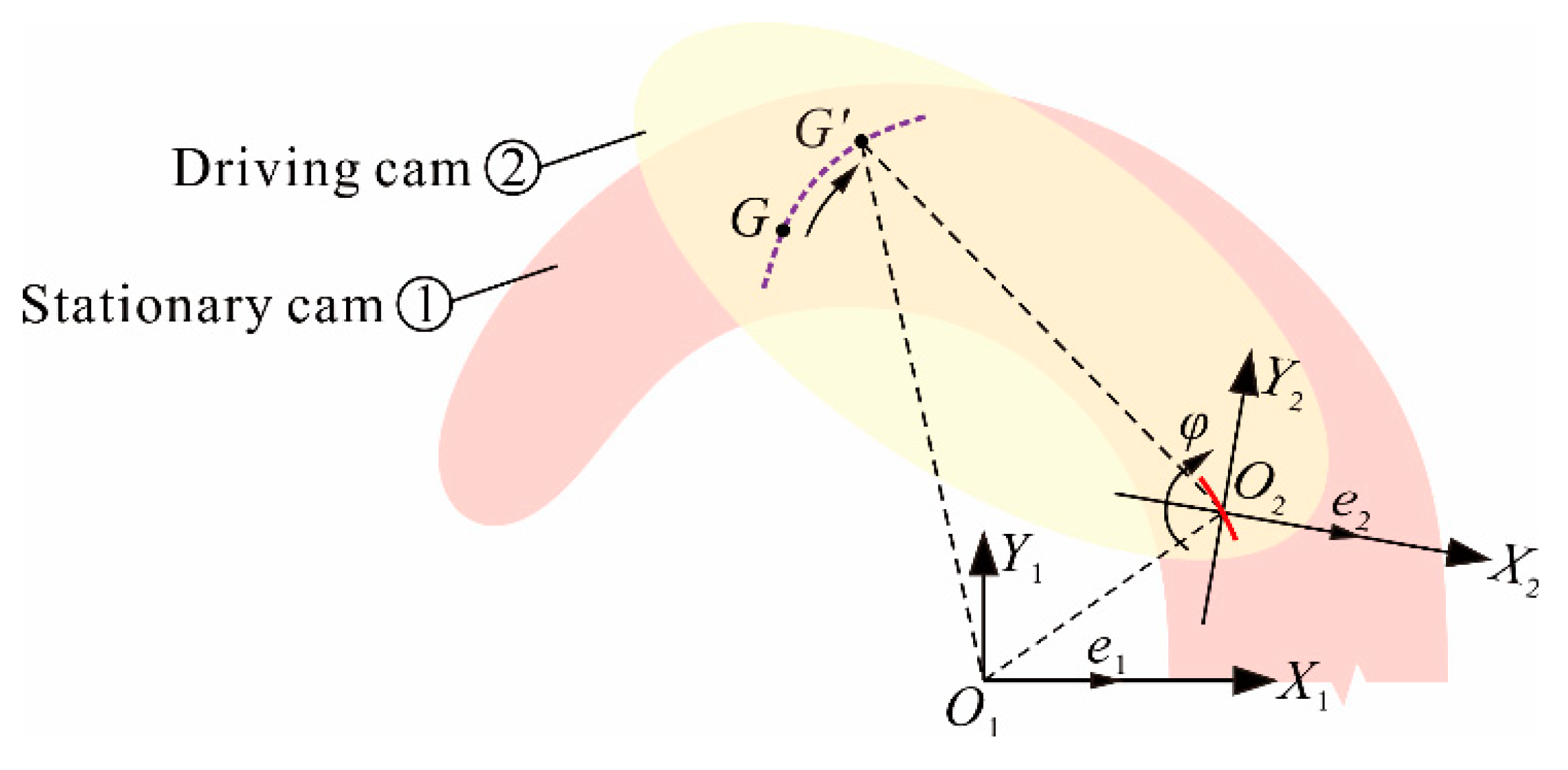
3.2.3. Motion Positioning Groove

Although the motion of driving cam is obtained in Section 3.2.2, the driving cam is not fully constrained. The base point O₂ only constrained one translational degree of freedom (DOF) of driving cam. The other two DOFs are the movement DOF of the base point O₂ along the No. j groove and the rotation DOF of the driving cam, which are not constrained. Except for the base point O₂, an additional positioning point G should be added to constrain the rotational DOF. Correspondingly, a motion positioning groove should be designed on stationary cam, whose pitch curve can be calculated by using obtained motion equations of the driving cam.

A coordinate system is shown in Figure 8. The additional motion positioning point G (X_2G, Y_2G) is on O₂-X₂Y₂ plane, the projection point of G on O₁-X₁Y₁ plane is G’ (X_1G’, Y_1G’). The trajectory of G’ forms the motion positioning groove.

If driving cam moves according to Equation (11), point G can form a projection trajectory on O₁-X₁Y₁ plane. With the driving cam rotates φ angle according to Equation (14), the projection of point G moves to point G’ on O₁-X₁Y₁ plane. According to coordinate transformation of Cartesian coordinate system, the coordinate of point G’ relative to O₂-X₂Y₂ plane is:

$$\left[\begin{array}{c}{X}_{1G’}\\ Y_{1G’}\end{array}\right]=\left[\begin{array}{cc}\cos \phi & -\sin \phi \\ \sin \phi & \cos \phi \end{array}\right]\left[\begin{array}{c}{X}_{2G}\\ Y_{2G}\end{array}\right]$$

(15)

So, the pitch curve of motion positioning groove is:

$$\{\begin{array}{c}{X}_{1G^{\prime }}=X_{2G}\cos \phi -Y_{2G}\sin \phi +(r+l)\cos \frac{jc}{r}-r\\ Y_{1G^{\prime }}=X_{2G}\sin \phi +Y_{2G}\cos \phi +(r+l)\sin \frac{jc}{r}\end{array}$$

(16)

The pitch curve of motion positioning groove and the final grooves of stationary cam are shown in Figure 9. All the grooves on lower half of stationary cam are symmetrical with upper half along X₁-axis on O₁-X₁Y₁ plane.

At this time, the rotation DOF of the driving cam is completely constrained by the motion positioning groove and the base point motion groove. We put pin shafts passes through these cam grooves corresponding to its serial number. The driving cam produces a relative motion with the stationary cam under an external driving force, their intersecting grooves interact to drives arc support linkages to move. Finally, the deployable arc can be continuously changed under the condition of maintaining its shape of an arc, and the mechanism has only one DOF, that is, the deployable arc can be deployed. A schematic diagram of the deploying process is shown in Figure 10.

3.3. Pitch Curve of Adjusting Groove

As shown in Figure 10, the deployable arc has been realized the deploying movement. However, the deployable arc is deployed centered on the midpoint of the arc, rather than centered on the circle center of the arc. Its deploying center point moves on the symmetrical center line. In order to solve this problem, it is necessary to add an adjusting groove. This section is to make the deployable arc have a fixed deployment center. The basic idea is to use an adjusting groove to drive a stationary cam to compensate for the displacement of a changing center. In this way, the mechanism can have a DOF for adjusting the deployment center. The stationary cam is placed on adjusting groove and move along with the direction of the linear guide located on the adjusting groove shown in Figure 1.

The coordinate system shown in Figure 3 is established when designing the pitch curves of stationary cam grooves. It can be seen from the figure that the deploying center point O always moves on X₁-axis, and there is no displacement is performed on Y₁-axis. If the endpoint R (X_1R, Y_1R) of any one of arc support linkage is selected as the driving point, the motion component Y_1R of point R on Y₁-axis is equal to the motion component Y_1P of point P on Y₁-axis in Equation (3). In the X₁-axis direction, it is only necessary to subtract the increment r of the arc radius change to keep the position of deploying center point O unchanged. According to the principle of relative motion, the relationship between X_1R and X_1P can be derived, that is, X_1R = X_1P − (−r). At this point, the pitch curve of the adjusting groove can be drawn:

$$\{\begin{array}{c}{X}_{1R}=(r+l)\cos \frac{ic}{r}\\ Y_{1R}=(r+l)\sin \frac{ic}{r}\end{array}$$

(17)

In this paper, we select the No. 1 pitch curve (i = 1 in Equation (17)) to design and produce adjusting groove. Make the pin shaft at the end of the No. 1 arc support linkage to passes through the No. 1 groove of the driving cam, stationary cam, and adjusting groove at the same time. Through the drive of the driving cam, the deployable arc profiling mechanism finally realizes the centering deployment around the circle center of the arc. Finally, the mechanism has two DOFs, one for deploying the deployable arc and the other for adjusting the deployment center. Figure 11 shows the difference between with and without adjusting groove, and a comparison of between centering and un-centering deploying motion.

3.4. Driving Parameter of Deployable Arc Profiling Mechanism

The driving component of the mechanism is composed of a push linkage and two equal length transmission linkages. The half-length of push linkage is s, the length of transmission linkage is t, as shown in Figure 12. The connection point between transmission linkage and driving cam is point U. The coordinate of point U on O₂-X₂Y₂ plane where the driving cam located is U (X_2U, Y_2U), and the projection point U’ of U on O₁-X₁Y₁ plane is U’ (X_1U’, Y_1U’) where the stationary cam located. The driving parameter is d.

It can be calculated from Equation (16), the coordinate of point U’ on O₁-X₁Y₁ plane is:

$$\{\begin{array}{c}{X}_{1U^{\prime }}=X_{2U}\cos \phi -Y_{2U}\sin \phi +(r+l)\cos \frac{jc}{r}-r\\ Y_{1U^{\prime }}=X_{2U}\sin \phi +Y_{2U}\cos \phi +(r+l)\sin \frac{jc}{r}\end{array}$$

(18)

Since the coordinate of point V (d, s), and the length of vector UV and U’V are equal to t on O₁-X₁Y₁ plane. Then the relationship between driving parameter d and arc radius r can be obtained as (d − X_1U’)² + (s − Y_1U’)² = t², solving it can get:

$$d=X_{1U^{\prime }}+\sqrt{t^2-{(s-Y_{1U^{\prime }})}^2}$$

(19)

Take Equation (18) into Equation (19), then the driving parameter d is finally obtained:

$$d=\sqrt{t^2-{\left[s-X_{2U}\sin \phi -Y_{2U}\cos \phi -(r+l)\sin \frac{jc}{r}\right]}^2}+X_{2U}\cos \phi -Y_{2U}\sin \phi +(r+l)\cos \frac{jc}{r}-r$$

(20)

In the end, all of the parameters of the deployable arc profiling mechanism were designed out. Among them, the pitch curve of stationary cam groove is Equation (3), the pitch curve of driving cam groove is Equation (10), the driving motion equation of driving cam are Equations (11) and (14), the pitch curve of motion positioning groove is Equation (16), the pitch curve of the adjusting groove is Equation (17), and the driving parameter is Equation (20).

4. Analysis and Experiment

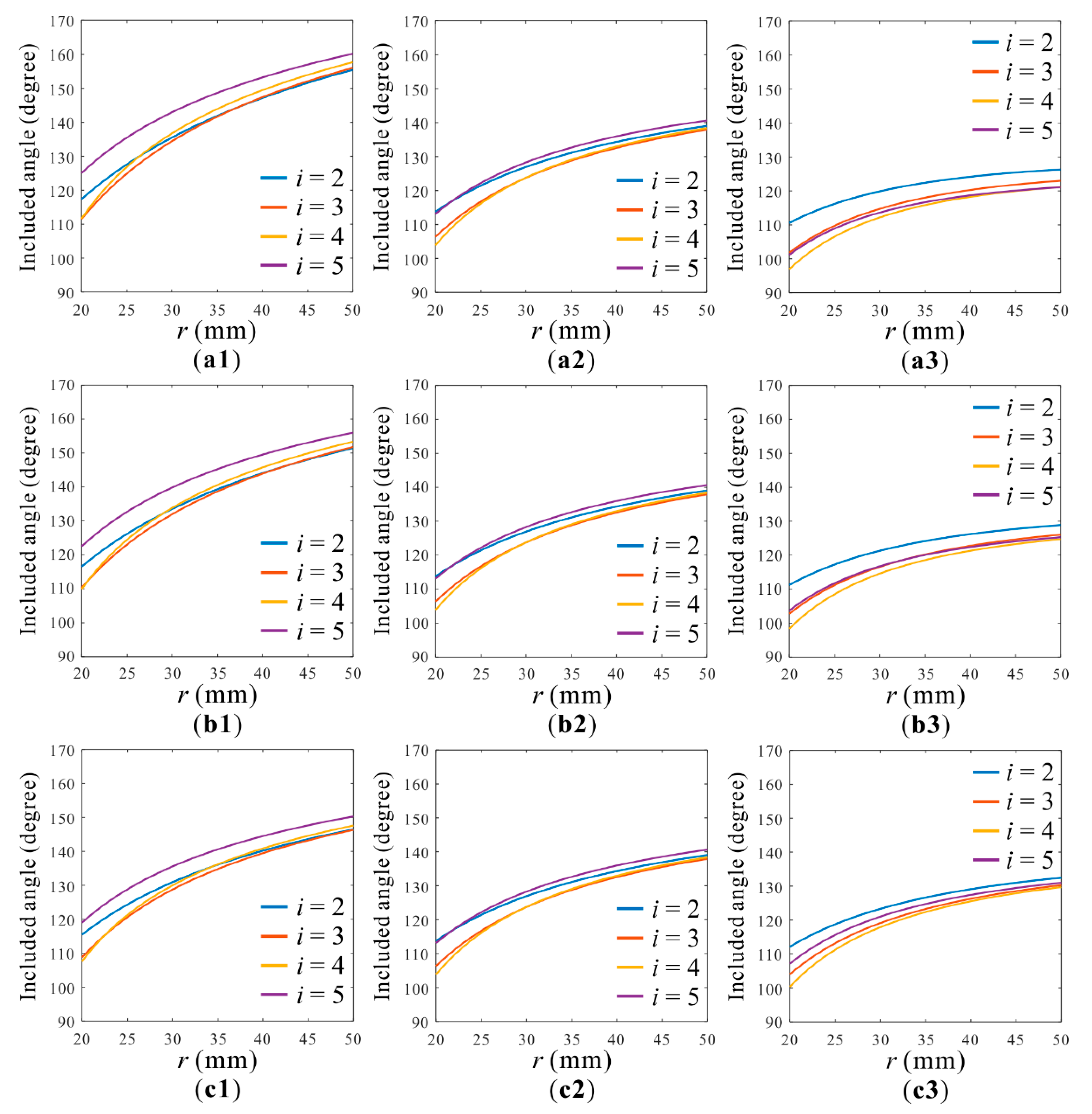
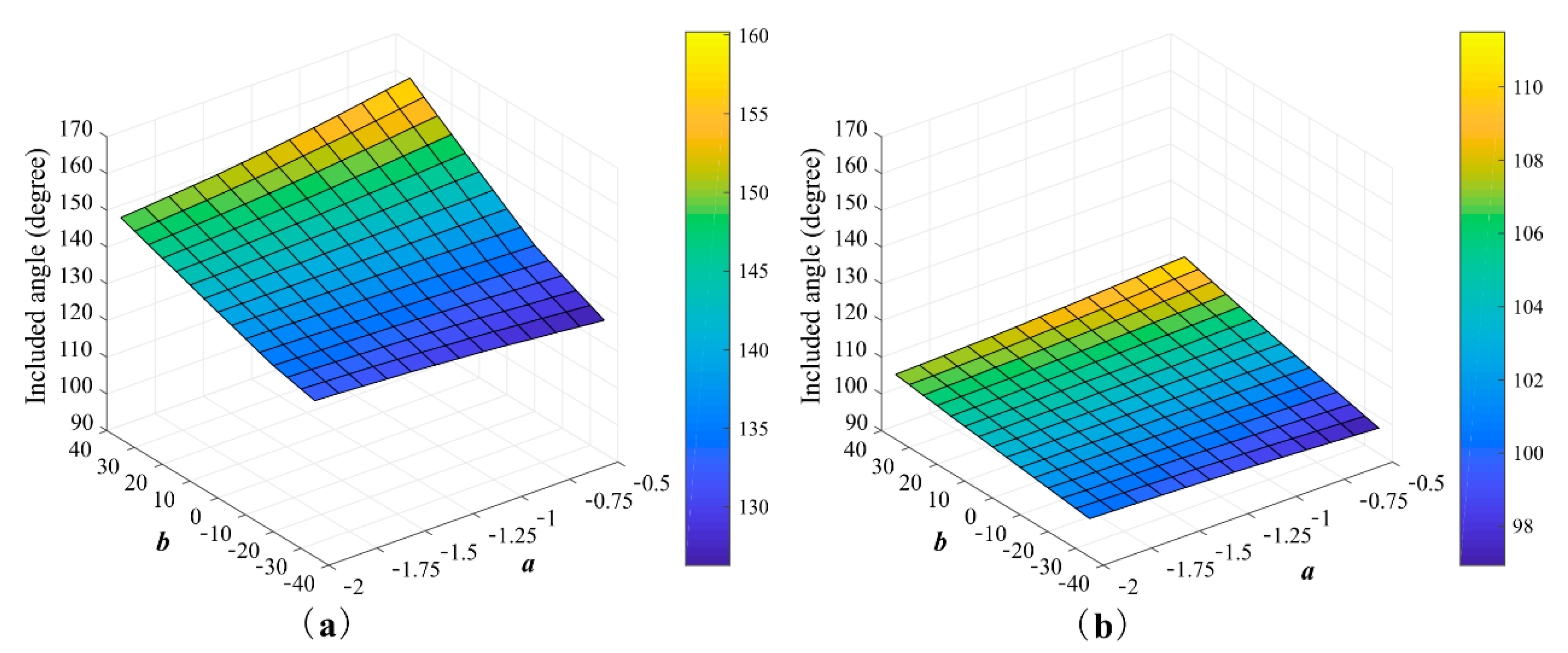
4.1. Impact of Parameters a and b

The movement of the pin shaft is driven by the intersecting groove between stationary cam and driving cam. There is an included angle of this intersecting groove shown in Figure 13. Due to the friction angle existing at the contact point between the pin shaft and groove, the value of the included angle could affect the movement of the pin shaft and the value of the driving force. In the design process of driving cam, we introduced a straight-line Y = aX + b, which is the key factor affecting the driving cam groove. Similarly, it affects the value of the included angle (variation range from 90° to 180°). In order to analyze the impact of parameters a and b on the included angle, we select a = −0.5, a = −1, and a = −2 in turn, corresponding to the value of each a, b = 35, b = 0, and b = −35 are sequentially selected for analysis. The other parameters in the analysis are r varies from 20 to 50 mm, l = 70 mm, c = 10 mm, j = 1, and n = 5. The results are shown in Figure 14.

It can be seen from the figure that as radius r increase, the included angle increases gradually. From the horizontal comparison of diagrams (a1), (a2), (a3), (b1), (b2), (b3), and (c1), (c2), (c3) can be seen that with the value of b decreases, the included angle decrease. From the longitudinal comparison of diagrams (a1), (b1), (c1), (a2), (b2), (c2), and (a3), (b3), (c3) can be seen that the value of a has little effect on the included angle. In particular, when b = 0, the change in the value of the included angle is no longer affected by a.

In the actual movement of the pin shaft, it could move smoothly in the intersecting groove under the condition that only when the value of maximum included angle minus 90° is always smaller than the friction angle. Therefore, we take the maximum value of the included angle to analyze the distribution law of the maximum value and the optimal parameter combination of a and b. For comparison, the minimum value of the included angle is also given. The results are shown in Figure 15.

From the figure, we can see that if the value of b is small, the value of the included angle gradually decreases with the increase of a. However, if the value of b is large, the value of the included angle gradually decreases with the decrease of a. If b = 0, the value of a has no effect on the included angle. Before and after this value, the variation trend of included angle changes with the value of a has changed. If a is fixed, then the included angle always decreases with the value of b decreases. Comparing (a) with (b), the variation trend of the maximum value and minimum value are the same, but the change of maximum value is greater. Within the selected test range, the optimal parameter combination of included angle is a = −0.5 and b = −35. For these parameters, the maximum value of the included angle is 126.3° and the minimum value is 96.9°.

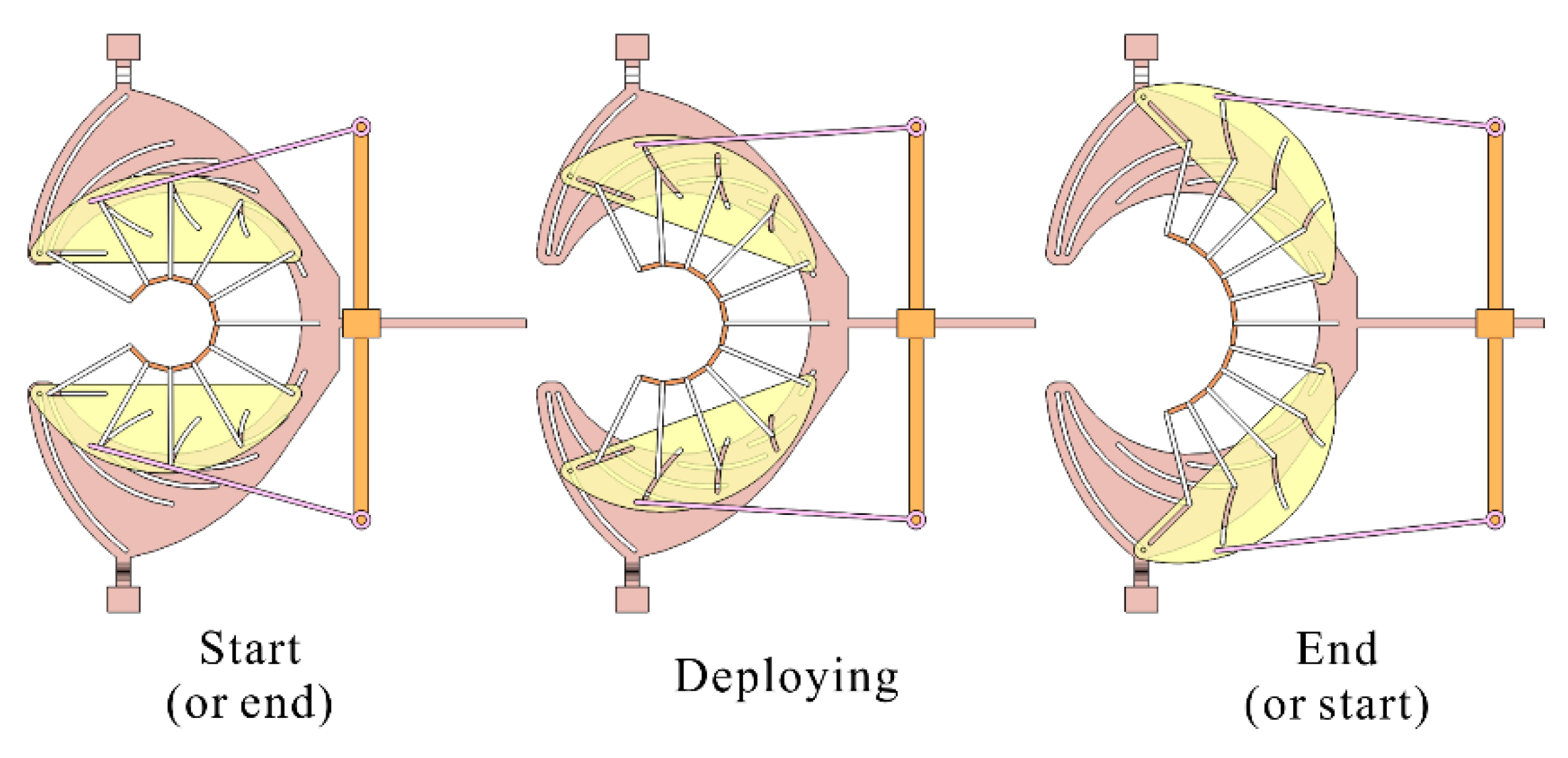
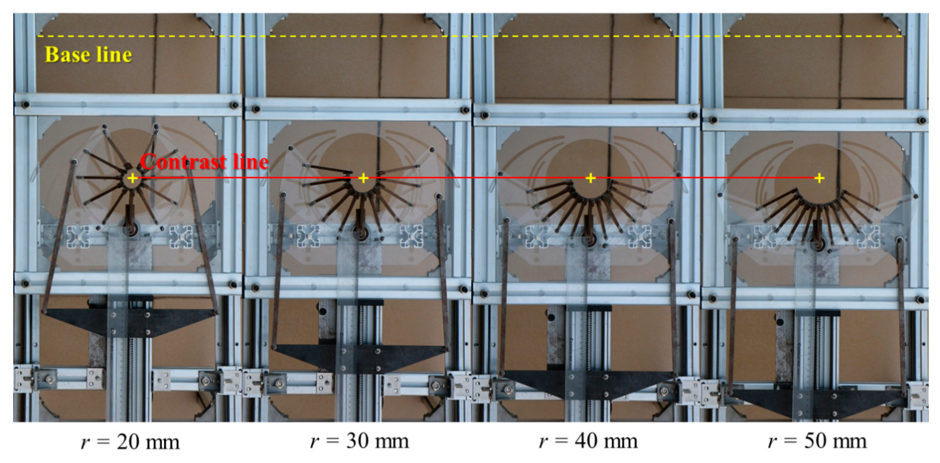
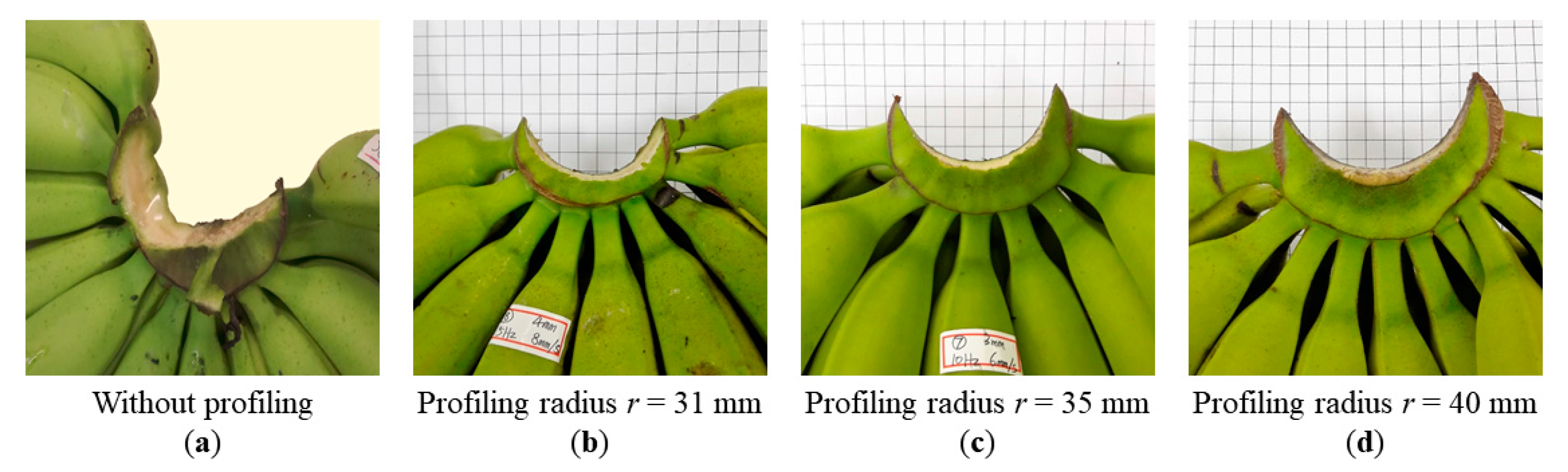
4.2. Prototype Verification

According to the pitch curves obtained by Equations (3), (10), (16), and (17), the grooves of each cam on experiment set of deployable arc profiling mechanism are processed. The experiment set uses a servomotor to drive the push linkage. The driving cam, stationary cam, and adjusting groove are all made of acrylic sheet. The selected processing parameters are listed in

Table 1. Processing parameters of experiment set.

Parameter	Value
Range of variation of radius r (mm)	20~50
Arc length of segment arc c (mm)	10.5
Length of arc support linkage l (mm)	70
Total number n of arc support linkages in upper part of mechanism	5
Length of push linkage s (mm)	150
Length of transmission linkage t (mm)	265
Given straight line	Y = −X/2 − 35
Coordinate of motion positioning point G	(−160, 43)
Coordinate of connecting point U	(−87, 79)

.

With the arc radius r varies from 20 to 50 mm, the driving parameter d is calculated from the Equation (20) that it varies from 213.7 to 328.6 mm. A number of values of arc radius are selected for testing. The diameter of the deployable arc is measured on the inner arc surface. The average diameter is calculated after four repeated measurements, and then converted to a radius value to be compared with the selected test value. The selected levels of test parameters and test results are listed in

Table 2. Selected levels of test parameters and test results.

Test Arc Radius r (mm)	Corresponding Parameter d (mm)	Measured Arc Radius r (mm)	Radius Deviation (mm)	Accuracy (%)
20	213.7	19.285	0.715	96.425
25	244.2	24.300	0.700	97.200
30	269.0	29.290	0.710	97.633
35	288.8	34.285	0.715	97.957
40	304.8	39.295	0.705	98.238
45	317.8	44.290	0.710	98.422
50	328.6	49.290	0.710	98.580

. Part of the deploying test process is shown in Figure 16.

From the test results, it can be seen that the radius deviation between the actual measured and the set value is maintained between 0.700 and 0.715 mm. Within the test range, the lowest value of profiling accuracy is 96.425% at 20 mm, and the highest value is 98.580% at 50 mm. With the gradual deploying of the arc, the profiling accuracy is gradually improved. From the deploying test process, it can be seen that regardless of how the radius of the arc changes, their center is always at a fixed point, which is the center of their arc. The variation range of the arc is very large, when the arc radius is small, the arc is nearly a circle.

In order to make the pin shaft move smoothly in the groove, the clearance fit method is adopted in the assembly between the groove and the pin shaft. Owing to the existence of clearance, the radius deviation occurred between the measured arc radius and the tested values [28,29,30]. With the test value is gradually increased, the accuracy of the experiment set is gradually increased. This is because the clearance value has a specific range, it almost unchanged during the test, the ratio between clearance value and test radius is gradually decreased, so the accuracy is gradually increased.

The test process shows that the mechanism can well achieve continuous profiling along a fixed center. This feature could be potentially used in banana crown cutting devices. The stalk of banana grows with bending and variable diameter, which requires the banana harvesting device to have a good function of profiling cutting with variable diameter. Therefore, we applied this deployable arc profiling mechanism to the banana crown cutting device to demonstrate its potential usage. Figure 17 shows the effect of the work after applying the deployable arc profiling mechanism. As a comparison, the working effect (Figure 17a) of a conventional cutting device that does not have such a deployable arc profiling mechanism is also exhibited. From the comparison, it can be seen that the working effect of the cutting device after the application is obviously better than that before. The incision quality of banana crown has greatly improved. The improvement of the quality of incision can increase the economic value of the banana, and prolong the preservation time. Therefore, the research and development of this mechanism has certain research value and application needs.

5. Conclusions

This paper proposed a novel symmetrical shape of deployable arc profiling mechanism that can be deployed around a fixed arc center and achieve continuous change of the arc radius. The mechanism is composed of compound cams, each cam contains multiple grooves. The deployable arc is driven for centering deployment through the interaction between driving cam grooves and stationary cam grooves, and through use, adjusting groove to adjust the displacement of deploying center point. By applying relative motion and inverse solution method, the pitch curve of each groove on each layer is designed, all the relevant equations of the mechanism are obtained.

The impact of the introduced straight-line Y = aX + b on the included angle of intersected grooves are also studied. We found that the value of b has a greater influence on the included angle, and the value of a has a smaller influence on it. If b = 0, the value of a has no effect on changes in the included angle. Within the selected test range, the maximum value of the included angle is 126.3°, and the minimum value is 96.9°.

The profiling accuracy of the deployable arc is studied by experiment. The results show that the radius deviation is maintained between 0.700 and 0.715 mm. The lowest value of profiling accuracy is 96.425%, and the highest value is 98.580%. With the deployment of the arc, the profiling accuracy is gradually improved. The potential usage of the deployable arc profiling mechanism is applied to the banana crown cutting device to demonstrate it. It is confirmed that the working effect of the cutting device after the application is obviously better than that before. The incision quality of the banana crown has greatly improved.

The straight line is used as an introduced curve to quickly design the pitch curve of the cam groove. In future work, by introducing different forms of curves to diversify the shape of the groove, and the included angle between these grooves can be further optimized.

6. Patent

The deployable arc profiling mechanism designed in this paper has applied for and obtained a Chinese invention patent, patent number: CN107598603A.

References

1. Abbas, A.T. A general algorithm for profiling and dressing grinding wheels when using a grinding spindle on a CNC lathe. Int. J. Prod. Res. 2004, 42, 3995–4008. [Google Scholar] [CrossRef]
2. Dudas, I.; Bodzas, S.; Dudas, I.S.; Mandy, Z. Development of spiroid worm gear drive having arched profile in axial section and a new technology of spiroid worm manufacturing with lathe center displacement. Int. J. Adv. Manuf. Technol. 2015, 79, 1881–1892. [Google Scholar] [CrossRef]
3. Wang, P.J.; Wu, Y.; Qi, J.F.; Chen, J.H.; Xiang, H. The development of special CNC system for profiling lathe based on digital capture measurement. Appl. Mech. Mater. 2013, 423, 2780. [Google Scholar] [CrossRef]
4. Liu, Z.Q.; Qiu, H.; Li, X.; Yang, S.L. Review of large spacecraft deployable membrane antenna structures. Chin. J. Mech. Eng. 2017, 30, 1447–1459. [Google Scholar] [CrossRef]
5. Dai, L.; Guan, F.L. Shape–sizing nested optimization of deployable structures using SQP. J. Cent. South Univ. 2014, 21, 2915–2920. [Google Scholar] [CrossRef]
6. Freeland, R.E.; Bilyeu, G.D.; Veal, G.R.; Steiner, M.D.; Carson, D.E. Large inflatable deployable antenna flight experiment results. Acta Astronaut. 1997, 41, 267–277. [Google Scholar] [CrossRef]
7. Hodges, R.E.; Chahat, N.; Hoppe, D.J.; Vacchione, J.D. A deployable high–gain antenna bound for mars developing a new folded–panel reflect array for the first CubeSat mission to mars. IEEE Antennas Propag. Mag. 2017, 59, 39–49. [Google Scholar] [CrossRef]
8. Chahat, N.; Sauder, J.; Hodges, R.E.; Thomson, M.; Rahmat–Samii, Y. The deep–space network telecommunication CubeSat antenna using the deployable Ka–band mesh reflector antenna. IEEE Antennas Propag. Mag. 2017, 59, 31–38. [Google Scholar] [CrossRef]
9. Ding, X.L.; Yang, Y.; Dai, J.S. Design and kinematic analysis of a novel prism deployable mechanism. Mech. Mach. Theory. 2013, 63, 35–49. [Google Scholar] [CrossRef]
10. Zeng, W.; Gao, F.; Jiang, H.; Huang, C.; Liu, J.X.; Li, H.F. Design and analysis of a compliant variable–diameter mechanism used in variable–diameter wheels for lunar rover. Mech. Mach. Theory. 2018, 125, 240–258. [Google Scholar] [CrossRef]
11. Feng, C.M.; Liu, T.S. A graph–theory approach to designing deployable mechanism of reflector antenna. Acta Astronaut. 2013, 87, 40–47. [Google Scholar] [CrossRef]
12. Feng, C.M.; Liu, T.S. A bionic approach to mathematical modeling the fold geometry of deployable reflector antennas on satellites. Acta Astronaut. 2014, 103, 36–44. [Google Scholar] [CrossRef]
13. Cao, W.A.; Yang, D.H.; Ding, H.F. Topological structural design of umbrella–shaped deployable mechanisms based on new spatial closed–loop linkage units. J. Mech. Des. 2018, 140, 062302. [Google Scholar] [CrossRef]
14. Huang, H.L.; Li, B.; Zhang, T.S.; Zhang, Z.; Qi, X.Z.; Hu, Y. Design of large single–mobility surface–deployable mechanism using irregularly shaped triangular prismoid modules. J. Mech. Des. 2019, 141, 012301. [Google Scholar] [CrossRef]
15. Figliolini, G.; Angeles, J. Synthesis of conjugate Geneva mechanisms with curved slots. Mech. Mach. Theory. 2002, 37, 1043–1061. [Google Scholar] [CrossRef]
16. Lee, J.J.; Cho, C.C. Improving kinematic and structural performance of Geneva mechanisms using the optimal control method. Proc. Inst. Mech. Eng. Part C-J. Eng. Mech. Eng. Sci. 2002, 216, 761–774. [Google Scholar] [CrossRef]
17. Lee, J.J.; Huang, K.F. Geometry analysis and optimal design of Geneva mechanisms with curved slots. Proc. Inst. Mech. Eng. Part C-J. Eng. Mech. Eng. Sci. 2004, 218, 449–459. [Google Scholar] [CrossRef]
18. Lee, J.J.; Jan, B.H. Design of Geneva mechanisms with curved slots for non–undercutting manufacturing. Mech. Mach. Theory. 2009, 44, 1192–1200. [Google Scholar] [CrossRef]
19. Ion, S.; Victor, M.; Liviu, C. On the Synthesis of Self Centering Grippers. In Proceedings of the NATO Advanced Study Institute Symposium on “Computational Methods in Mechanisms”, Varna, Bulgaria, 16 June 1997; Kluwer Academic Publishers: Dordrecht, The Netherlands, 1997. [Google Scholar]
20. Ion, S.; Ion, I. Mathematical models of grippers. In Proceedings of the 10th WSEAS International Conference on Mathematical and Computational Methods in Science and Engineering, Corfu, Greece, October 26 2008; WSEAS Press: Stevens Point, WI, USA, 2008. [Google Scholar]
21. Ion, S.; Cătalin, I. Optimum design of self centering grippers. U.P.B. Sci. Bull. Series D. 2011, 73, 43–52. [Google Scholar]
22. Chen, J.H.; Lin, Z.; Wu, Y.J. Design of cylindrical cam with oscillating follower based on 3D expansion of planar profile model. Chin. J. Mech. Eng. 2009, 22, 665–670. [Google Scholar] [CrossRef]
23. Soong, R.C. A new cam–geared mechanism for exact path generation. J. Adv. Mech. Des. Syst. Manuf. 2015, 9, 15–00144. [Google Scholar] [CrossRef]
24. Soong, R.C. A cam–geared mechanism for rigid body guidance. Trans. Can. Soc. Mech. Eng. 2017, 41, 143–157. [Google Scholar] [CrossRef]
25. Todd, G.N.; Robert, J.L.; Spencer, P.M.; Larry, L.H. Curved–folding–inspired deployable compliant rolling–contact element (D–CORE). Mech. Mach. Theory. 2016, 96, 225–238. [Google Scholar] [CrossRef]
26. Zhou, C.J.; Hu, B.; Chen, S.Y.; Ma, L. Design and analysis of high–speed cam mechanism using Fourier series. Mech. Mach. Theory. 2016, 104, 118–129. [Google Scholar] [CrossRef]
27. Li, M.; Wang, R.X.; Zhao, Z.H. Passive nonlinear actuators for deploying mesh antennas. Acta Astronaut. 2018, 152, 254–261. [Google Scholar] [CrossRef]
28. Li, J.L.; Yan, S.Z.; Guo, F.; Guo, P.F. Effects of damping, friction, gravity, and flexibility on the dynamic performance of a deployable mechanism with clearance. Proc. Inst. Mech. Eng. Part C-J. Eng. Mech. Eng. Sci. 2013, 227, 1791–1803. [Google Scholar] [CrossRef]
29. Sanmiguel, R.E.; Hidalgo, M.M. Cam mechanisms based on a double roller translating follower of negative radius. Mech. Mach. Theory. 2016, 95, 93–101. [Google Scholar] [CrossRef]
30. Ye, H.L.; Zhang, Y.; Yang, Q.S.; Xiao, Y.N.; Ramana, V.G.; Christopher, C.F. Optimal design of a three tape–spring hinge deployable space structure using an experimentally validated physics–based model. Struct. Multidiscip. Optim. 2017, 56, 973–989. [Google Scholar] [CrossRef]
Figure 1. Structure of deployable arc profiling mechanism.
Symmetry 11 00958 g001
Figure 2. Deploying process and arc support linkage number.
Symmetry 11 00958 g002
Figure 3. Coordinate system of stationary cam.
Symmetry 11 00958 g003
Figure 4. Pitch curves of stationary cam grooves and upper part of stationary cam.
Symmetry 11 00958 g004
Figure 5. Coordinate system of driving cam.
Symmetry 11 00958 g005
Figure 6. Pitch curves of driving cam grooves and upper part of driving cam.
Symmetry 11 00958 g006
Figure 7. Coordinate system of rotational motion.
Symmetry 11 00958 g007
Figure 8. Coordinate system of motion positioning groove.
Symmetry 11 00958 g008
Figure 9. Pitch curve of motion positioning groove and final grooves of stationary cam.
Symmetry 11 00958 g009
Figure 10. Schematic diagram of deploying process.
Symmetry 11 00958 g010
Figure 11. Comparison of between centering and un-centering deploying motion.
Symmetry 11 00958 g011
Figure 12. Coordinate system of driving motion.
Symmetry 11 00958 g012
Figure 13. Included angle of intersecting groove.
Symmetry 11 00958 g013
Figure 14. Impact of parameters a and b on included angle. (a1) a = −0.5, b = 35, (a2) a = −0.5, b = 0, (a3) a = −0.5, b = −35, (b1) a = −1, b = 35, (b2) a = −1, b = 0, (b3) a = −1, b = −35, (c1) a = −2, b = 35, (c2) a = −2, b = 0, (c3) a = −2, b = −35.
Symmetry 11 00958 g014
Figure 15. Distribution law of maximum and minimum value of included angle. (a) Maximum value of included angle, (b) Minimum value of included angle.
Symmetry 11 00958 g015
Figure 16. Part of the deploying test process.
Symmetry 11 00958 g016
Figure 17. Comparison of incision quality between without and with application of deployable arc profiling mechanism.
Symmetry 11 00958 g017