Automatically Detecting Excavator Anomalies Based on Machine Learning


Abstract
:1. Introduction
2. Related Work
- Expert systems [2,3,4]. To detect excavator anomalies, the authors in [2] discussed an expert system framework for failure detection and predictive maintenance (FDPM) of a mine excavator. FDPM includes an expert system engine and a mathematical knowledge base for fault detection and the corresponding repairing under various conditions. However, the authors in [2] only proposed a framework without implementation, so the effectiveness has not been validated. The authors in [3,4] combined the fault tree analysis with simple rule-based expert system, and designed an expert system with complex reasoning and interpretation functions. However, the construction of the fault tree and the latter analysis highly rely on the professional domain knowledge in a specific environment, which may not be easily adopted to general excavators.
- Traditional statistic models [5,6,7]. These methods mainly use traditional probability and statistics algorithms for anomaly detection. For instance, the authors in [5,6] rely on principal component analysis (PCA) and auto-regressive with extra output (ARX) to extract features that reflect anomalies, and fuzzy c-means (FCM) and radial basis function (RBF) to cluster anomalies and norms, respectively. However, these methods are shown to be not effective when applying to complex and large-volume multi-sensor data. Moreover, the authors in [5,6] only carried out experiments using simulated dataset but no real data verification. The authors in [7] proposed a framework for excavator fault diagnosis based on multi-agent system (MAS). However, only the overall design has been presented and their system has not been implemented and verified.
3. Data Sources
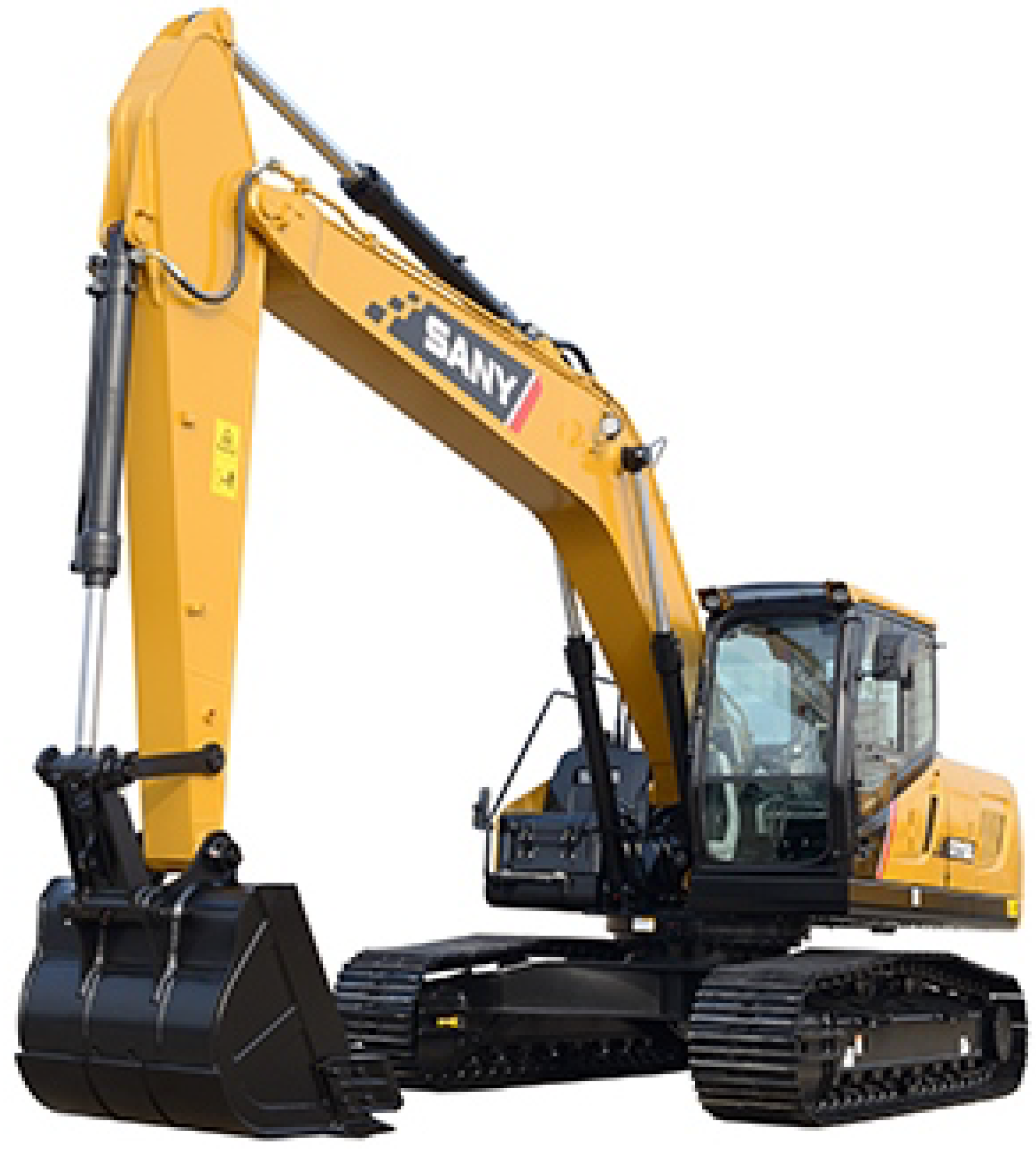
3.1. Excavator Description
3.2. Data Collection
4. Data Preprocessing
4.1. Cleaning Data
4.2. Labeling Anomalies
5. Methodology
5.1. Merging Time-Series into Discrete Samples
5.2. Feature Selection
5.2.1. Association Rule Mining Based on an a Priori Algorithm
5.2.2. Using Association Rules to Select Features
5.3. Anomaly Detection Algorithms for Excavators
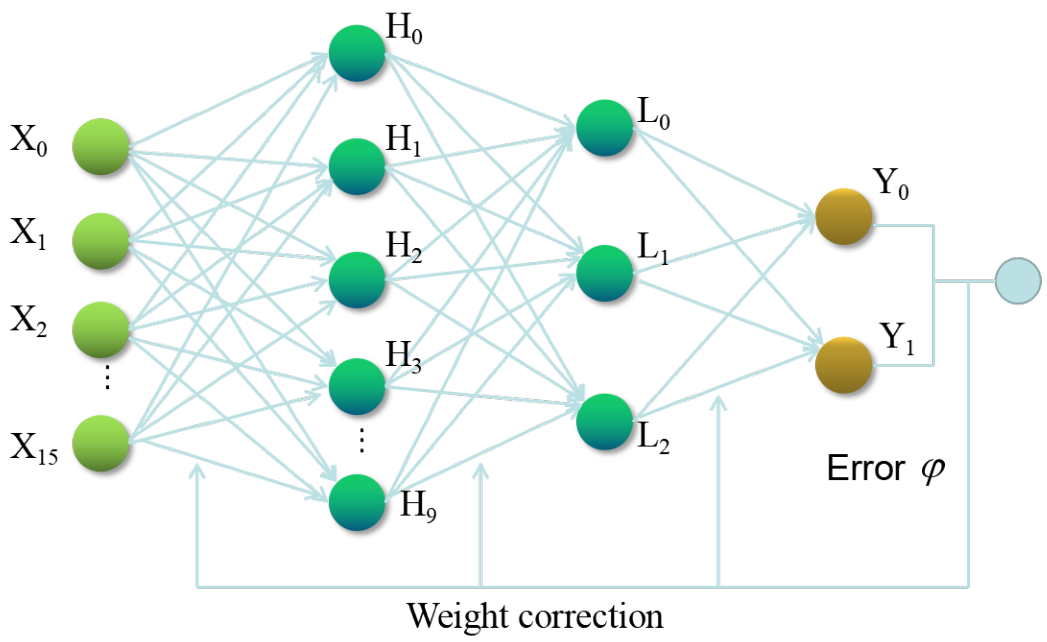
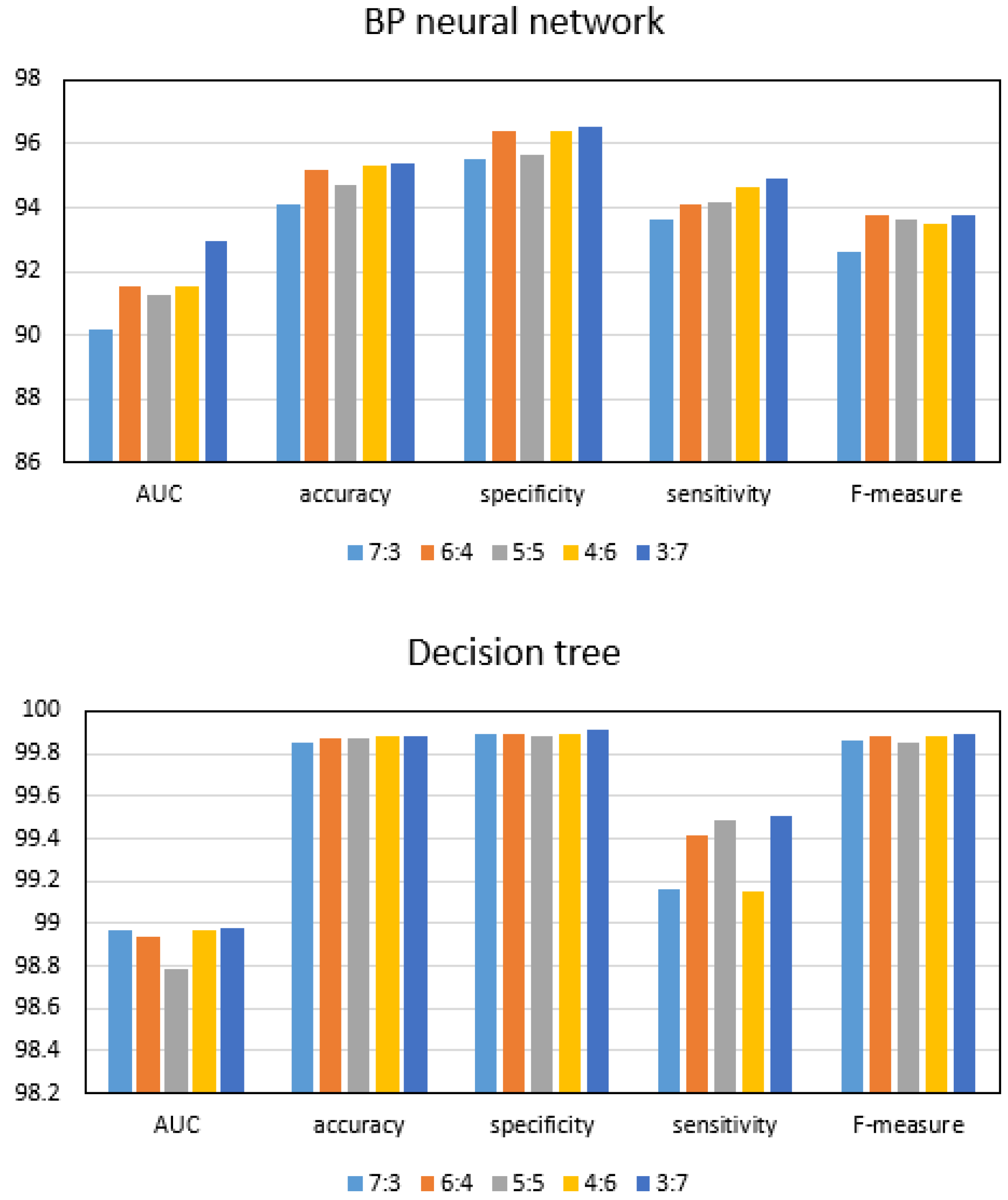
5.3.1. BP Neural Network-Based Anomaly Detection
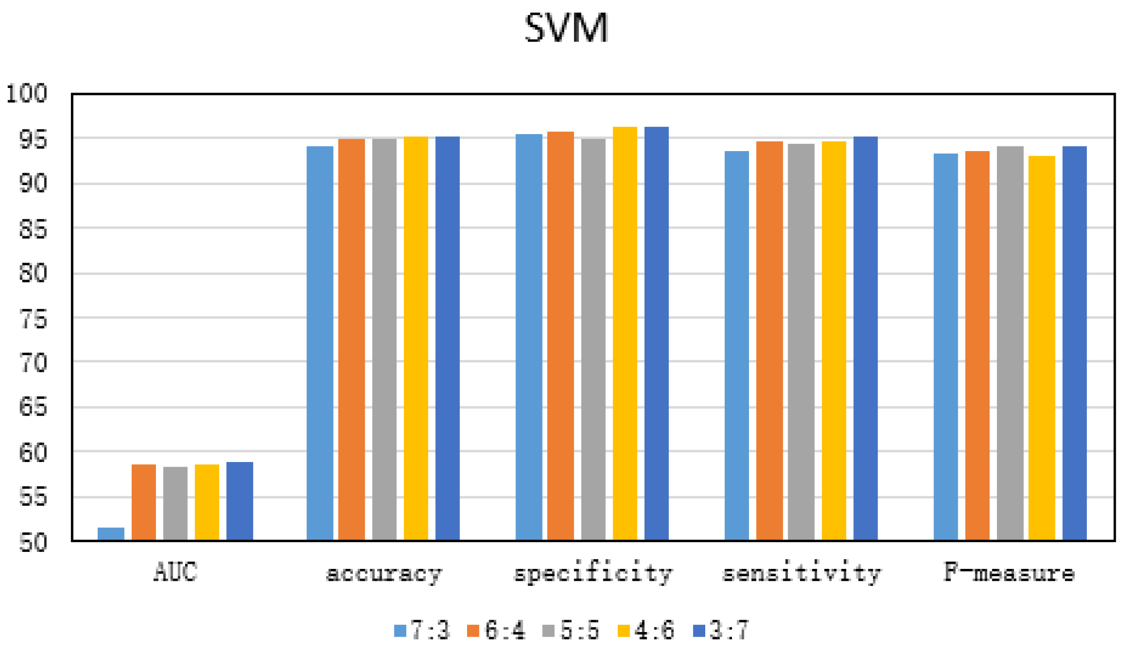
5.3.2. SVM-Based Anomaly Detection
5.3.3. Decision Tree-Based Anomaly Detection
6. Experimental Analysis
6.1. Evaluation Metrics
6.2. Comprehensive Evaluation
6.2.1. Exploring the Optimal Ratio of Test Set to Training Set
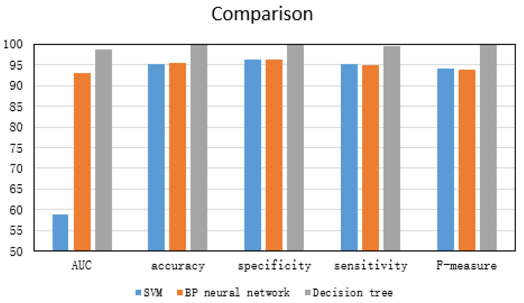
6.2.2. Performance Evaluation of Three Anomaly Detection Methods
7. Conclusions
Author Contributions
Funding
Conflicts of Interest
Abbreviations
| SVM | Support vector machine |
| BP | Back propagation |
| ML | Machine learning |
| FDPM | Failure detection and predictive maintenance |
| PCA | Principal component analysis |
| ARX | Auto-regressive with extra output |
| FCM | Fuzzy c-means |
| RBF | Radial basis function |
| MAS | Multi-agent system |
| CAN | Controller area network |
| SRM | Structural risk minimization |
| SVs | Support vectors |
| AUC | Area under ROC curve |
References
- SY215C Medium Hydraulic Excavator. Available online: http://product.sanygroup.com/zw-sy215c-10.html (accessed on 6 May 2019).
- Kumar, P.; Srivastava, R. An expert system for predictive maintenance of mining excavators and its various forms in open cast mining. In Proceedings of the 2012 1st International Conference on Recent Advances in Information Technology (RAIT), Dhanbad, India, 15–17 March 2012; pp. 658–661. [Google Scholar] [CrossRef]
- Yin, J.; Mei, L. Fault Diagnosis of Excavator Hydraulic System Based on Expert System. Lect. Notes Electr. Eng. 2011, 122, 87–92. [Google Scholar]
- Li, G.; Zhang, Q. Hydraulic fault diagnosis expert system of excavator based on fault tree. Adv. Mater. Res. 2011, 228, 439–446. [Google Scholar] [CrossRef]
- He, X.; He, Q. Application of PCA method and FCM clustering to the fault diagnosis of excavator’s hydraulic system. IEEE Int. Conf. Autom. Lofistics 2007, 1635–1639. [Google Scholar] [CrossRef]
- He, X. Fault Diagnosis of Excavator’s Hydraulic System Based on ARX Model. In Proceedings of the International Conference on Mechanical Design, Manufacture and Automation Engineering, Phuket, Thailand, 11–12 June 2014. [Google Scholar]
- Tang, X.Y.; Cui, Y.J.; Zhou, M.; Li, J.X. Study on MAS-Based Fault Diagnosis System for GJW111 Excavator. Adv. Mater. Res. 2012, 497, 1946–1949. [Google Scholar] [CrossRef]
- Lu, Y.; Chen, G.; Li, B.; Tan, K.; Xiong, Y.; Cheng, P.; Zhang, J.; Chen, E.; Moscibroda, T. Multi-Path Transport for RDMA in Datacenters. In Proceedings of the 15th USENIX Symposium on Networked Systems Design and Implementation (NSDI 18), Renton, WA, USA, 9–11 April 2018; USENIX Association: Renton, WA, USA, 2018; pp. 357–371. [Google Scholar]
- Chen, G.; Lu, Y.; Meng, Y.; Li, B.; Tan, K.; Pei, D.; Cheng, P.; Luo, L.L.; Xiong, Y.; Wang, X.; et al. Fast and Cautious: Leveraging Multi-path Diversity for Transport Loss Recovery in Data Centers. In Proceedings of the 2016 USENIX Annual Technical Conference (USENIX ATC 16), Denver, CO, USA, 20–21 June 2016; USENIX Association: Denver, CO, USA, 2016; pp. 29–42. [Google Scholar]
- Lu, Y.; Chen, G.; Luo, L.; Tan, K.; Xiong, Y.; Wang, X.; Chen, E. One more queue is enough: Minimizing flow completion time with explicit priority notification. In Proceedings of the IEEE INFOCOM 2017—IEEE Conference on Computer Communications, Atlanta, GA, USA, 1–4 May 2017; pp. 1–9. [Google Scholar] [CrossRef]
- Chen, J.; Li, K.; Tang, Z.; Bilal, K.; Yu, S.; Weng, C.; Li, K. A Parallel Random Forest Algorithm for Big Data in a Spark Cloud Computing Environment. IEEE Trans. Parallel Distrib. Syst. 2017, 28, 919–933. [Google Scholar] [CrossRef]
- Chen, J.; Li, K.; Deng, Q.; Li, K.; Yu, P.S. Distributed Deep Learning Model for Intelligent Video Surveillance Systems with Edge Computing. IEEE Trans. Ind. Inf. 2019. [Google Scholar] [CrossRef]
- Duan, M.; Li, K.; Liao, X.; Li, K. A Parallel Multiclassification Algorithm for Big Data Using an Extreme Learning Machine. IEEE Trans. Neural Netw. Learn. Syst. 2018, 29, 2337–2351. [Google Scholar] [CrossRef]
- D’Angelo, G.; Palmieri, F.; Rampone, S. Detecting unfair recommendations in trust-based pervasive environments. Inf. Sci. 2019, 486, 31–51. [Google Scholar] [CrossRef]
- Sanygroup. Available online: http://www.sanygroup.com/ (accessed on 6 May 2019).
- Vapnik, V.; Lerner, A. Recognition of Patterns with help of Generalized Portraits. Avtomat. I Telemekh 1963, 24, 774–780. [Google Scholar]
- Rumelhart, D.; Hinton, G.; Williams, R. Learning representations by back-propagating errors. Nature 1986, 323, 533–536. [Google Scholar] [CrossRef]
- Rokach, L.; Maimon, O. Data Mining with Decision Trees: Theory and Applications; World Scientific: Singapore, 2008. [Google Scholar]
- Chiba, Z.; Abghour, N.; Moussaid, K.; Omri, A.; Rida, M. A Hybrid Optimization Framework Based on Genetic Algorithm and Simulated Annealing Algorithm to Enhance Performance of Anomaly Network Intrusion Detection System Based on BP Neural Network. In Proceedings of the 2018 International Symposium on Advanced Electrical and Communication Technologies (ISAECT), Kenitra, Morocco, 21–23 November 2018; pp. 1–6. [Google Scholar] [CrossRef]
- Shan, Y.; Yijuan, L.; Fangjing, G. The Application of BP Neural Network Algorithm in Optical Fiber Fault Diagnosis. In Proceedings of the 2015 14th International Symposium on Distributed Computing and Applications for Business Engineering and Science (DCABES), Guiyang, China, 18–24 August 2015; pp. 509–512. [Google Scholar] [CrossRef]
- Lei, Y. Network Anomaly Traffic Detection Algorithm Based on SVM. In Proceedings of the 2017 International Conference on Robots & Intelligent System (ICRIS), Huai’an, China, 15–16 October 2017; pp. 217–220. [Google Scholar] [CrossRef]
- Zhang, M.; Xu, B.; Gong, J. An Anomaly Detection Model Based on One-Class SVM to Detect Network Intrusions. In Proceedings of the 2015 11th International Conference on Mobile Ad-hoc and Sensor Networks (MSN), Shenzhen, China, 16–18 December 2015; pp. 102–107. [Google Scholar] [CrossRef]
- Chaaya, G.; Maalouf, H. Anomaly detection on a real-time server using decision trees step by step procedure. In Proceedings of the 2017 8th International Conference on Information Technology (ICIT), Amman, Jordan, 17–18 May 2017; pp. 127–133. [Google Scholar] [CrossRef]
- Feng, Z.; Hongsheng, S. A decision tree approach for power transformer insulation fault diagnosis. In Proceedings of the 2008 7th World Congress on Intelligent Control and Automation, Chongqing, China, 25–27 June 2008; pp. 6882–6886. [Google Scholar] [CrossRef]
- Cherkasskey, V. The nature of statistical learning theory. IEEE Trans. Neural Netw. 1997, 8, 1564. [Google Scholar] [CrossRef] [PubMed]
- Vapnik, V.; Vapnik, V. Statistical Learning Theory; Wiley: New York, NY, USA, 1998. [Google Scholar]
- Vapnik, V.; Vapnik, V. An overview of statistical learning theory. IEEE Trans. Neural Netw. 1999, 10, 988–999. [Google Scholar] [CrossRef] [PubMed]
- Chen, X.; Xu, L.; Liu, X.; Wang, X. Application of Decision-tree Algorithm in Equipment Fault Detection. Ordnance Ind. Autom. 2015, 10, 81–84. [Google Scholar]


| Item | Description |
|---|---|
| Size of the dataset | 2,998,690 |
| The number of sampled metrics | 68 |
| Time span of data collection | 40 days |
| Excavator model | SY215C |
| Number of excavators | 107 |
| Indexes | Character Representation | Brief Description | Type |
|---|---|---|---|
| Number of GPS satellites | Gps_starsnum | The number of GPS satellites | Numeric |
| GPRS signal strength | Gprs_sigstrength | The strength of the GPRS signal | Numeric |
| GPRSEMEI no. | Gprs_emei | The serial number of GPRSEMEI | Numeric |
| Local data acquisition time | Timestamp_local | Data collection time of the equipment | Numeric |
| Device data entry time | Timestamp_cloudm2m | The time when the data enters the cloud | Numeric |
| Device ID | Deviceid | The ID number of the device | Numeric |
| Major key ID | Uuid | The major key ID number of the device | Numeric |
| Date | Bizdate | Date of data collection | Numeric |
| Indexes | Character Representation | Brief Description | Type |
|---|---|---|---|
| Equipment GPSID | Gpsid | The device is configured with the GPS ID | Numeric |
| Device IP address | Ip | IP address of the device | Numeric |
| Time | Time | Data acquisition time | Numeric |
| GPS status | Rd_gpssta | Shows the current status of the GPS | Numeric |
| TRU system fault word_word fault code | Rd_werrorcode | Indicates whether the device is faulty | Numeric |
| TRU alarm combination word_word alarm code | Rd_walmcode | Show whether the device has an alarm | Numeric |
| Gear position | Rd_steppos | Display device working gear | Numeric |
| HCU alarm merge word 1_bit fault code | Rd_berrorcode | Displays the specific fault type | Numeric |
| HCU alarm merge word 2_bit alarm code | Rd_balmcode | Displays the specific alarm type | Numeric |
| HCU system fault word_number of satellites | Rd_saticunt | Show the number of satellites | Numeric |
| Action number_fault handling status | Rd_errdealsta | Shows whether the fault has been handled | Numeric |
| Handshake switch | rd_commctsch | Used to display handshake switches | Numeric |
| Operating mode | Rd_uintresv10 | Show what mode of operation the device is in | Numeric |
| Display operates the switch quantity | Rd_uintresv11 | Operating switch value of display screen | Numeric |
| Input switch | Rd_uintresv12 | Switches collected by sensors | Numeric |
| Output switch | Rd_uintresv13 | Variable of electrical component output | Numeric |
| Lock machine level | Rd_uintresv14 | Displays the lock level | Numeric |
| Cell phone number 1_3 digits | Rd_uintresv15 | Display the phone number 1–3 digits | Numeric |
| Cell phone number 4_7 digits | Rd_uintresv16 | Display the phone number 4–7 digits | Numeric |
| Cell phone number 8_11 digits | Rd_uintresv17 | Display the phone number 8–11 digits | Numeric |
| Call status word | Rd_uintresv18 | Shows what call state it is in | Numeric |
| Call instruction | Rd_uintresv19 | Display call command | Numeric |
| Noload engine speed | Rd_uintresv20 | Engine speed at which the equipment is idle | Numeric |
| The largest stall | Rd_uintresv21 | Shows maximum engine stall | Numeric |
| Average stall | Rd_uintresv22 | Show engine average speed | Numeric |
| Screen application version number | Rd_uintresv23 | The version number used by the device | Numeric |
| Longitude 1 | Rd_longitude | Displays the longitude 1 of the device | Numeric |
| Latitude 1 | Rd_latitude | Displays the latitude 1 of the device | Numeric |
| Displacement velocity 1 | Rd_velocity | Operating speed 1 of equipment (km/h) | Numeric |
| Displacement direction 1 | Rd_orientation | The displacement direction 1 of the device | Numeric |
| Working time | Rd_wktime | Last startup time of the equipment | Numeric |
| Total working time | Rd_totalwktime | Total working hours of the equipment | Numeric |
| Lock machine remaining time | Rd_rmntime | The remaining time of the device being locked | Numeric |
| Battery voltage | Rd_batteryvol | Display battery voltage | Numeric |
| Engine speed | Rd_engv | Display engine speed | Numeric |
| Fuel oil level | Rd_oillev | Fuel level of equipment (%) | Numeric |
| Height | Rd_altitude | Altitude of the equipment | Numeric |
| Signal quality | Rd_sgniq | Shows the strength of satellite signal quality | Numeric |
| Cooling water temperature | Rd_floatresv13 | Display cooling water temperature | Numeric |
| Pump 1 main pressure | Rd_floatresv14 | Display pump 1 main pressure size | Numeric |
| Pump 2 main pressure | Rd_floatresv15 | Display pump 2 main pressure size | Numeric |
| Proportional valve 1 current | Rd_floatresv16 | The current level of proportional valve 1 | Numeric |
| Proportional valve 2 current | Rd_floatresv17 | The current level of proportional valve 2 | Numeric |
| Oil pressure | Rd_floatresv18 | Display oil pressure | Numeric |
| Hydraulic oil temperature | Rd_floatresv19 | Display the temperature of the hydraulic oil | Numeric |
| Action time_arm lift | Rd_floatresv20 | Pilot pressure for arm lift | Numeric |
| Fuel consumption_arm drop | Rd_floatresv21 | Lead pressure for arm drop | Numeric |
| Front pump mean main pressure | Rd_floatresv22 | Front pump average main pressure size | Numeric |
| Front pump average current | Rd_floatresv23 | Front pump solenoid valve average current size | Numeric |
| Front pump average power | Rd_floatresv24 | Display front pump average power | Numeric |
| Mean main pressure of rear pump | Rd_floatresv25 | The average main pressure of the rear pump | Numeric |
| Rear pump average current | Rd_floatresv26 | Display the average current of the rear pump | Numeric |
| Average power of rear pump | Rd_floatresv27 | Display the average power of the rear pump | Numeric |
| Throttle voltage | Rd_floatresv28 | Voltage at the throttle of the device | Numeric |
| Gear voltage | Rd_floatresv29 | Display the voltage level of each gear | Numeric |
| Longitude | Gps_longitude | Displays the longitude of the device | Numeric |
| Latitude | Gps_latitude | Displays the latitude of the device | Numeric |
| The displacement speed | Gps_velocity | Operating speed of equipment (km/h) | Numeric |
| Sense of displacement | Gps_orientation | The displacement direction of the device | Numeric |
| GPS signal strength | Gps_sigstrength | The strength of the GPS signal | Numeric |
| Feature | Character Representation | Brief Description | Type |
|---|---|---|---|
| Gear position | Rd_steppos | Display device working gear | Numeric |
| Operating mode | Rd_uintresv10 | Show what mode of operation the device is in | Numeric |
| Output switch | Rd_uintresv13 | Variable of electrical component output | Numeric |
| Average stall | Rd_uintresv22 | Show engine average speed | Numeric |
| Total working time | Rd_totalwktime | Total working hours of the equipment | Numeric |
| Battery voltage | Rd_batteryvol | Display battery voltage | Numeric |
| Engine speed | Rd_engv | Display engine speed | Numeric |
| Cooling water temperature | Rd_floatresv13 | Display cooling water temperature | Numeric |
| Pump 1 main pressure | Rd_floatresv14 | Display pump 1 main pressure size | Numeric |
| Pump 2 main pressure | Rd_floatresv15 | Display pump 2 main pressure size | Numeric |
| Proportional valve 1 current | Rd_floatresv16 | Display the current level of proportional valve 1 | Numeric |
| Proportional valve 2 current | Rd_floatresv17 | Display the current level of proportional valve 2 | Numeric |
| hydraulics pressure | Rd_floatresv18 | Display oil pressure | Numeric |
| Hydraulic oil temperature | Rd_floatresv19 | Display the temperature of the hydraulic oil | Numeric |
| Throttle voltage | Rd_floatresv28 | Voltage at the throttle of the device | Numeric |
| Gear voltage | Rd_floatresv29 | Display the voltage level of each gear | Numeric |
| Parameter | Description | Value |
|---|---|---|
| net.trainmethod | training method | traingd |
| net.trainParam.epochs | Maximum number of training | 10 |
| net.trainParam.goal | Training requirements accuracy | 0 |
| net.trainParam.lr | Learning rate | 0.01 |
| net.trainParam.max_fail | Maximum number of failures | 6 |
| Parameter | Description | Value |
|---|---|---|
| C | Penalty coefficient of the objective function | 1 |
| Kernel | Kernel function | RBF |
| Gamma | Kernel function bandwidth | 1/16 |
| Coef0 | Independent item in the kernel function | 0 |
| Probablity | Specify whether to use probability estimation when predicting a decision | False |
| Class_weight | Refers to the weight of each class | 1 |
| Max_iter | The maximum number of iterations | −1 |
| Parameter | Description | Value |
|---|---|---|
| Criterion | Feature selection criteria | Entropy |
| Splitter | Character classification criteria | Best |
| Max_depth | Maximum depth of decision tree | None |
| Min_impurity_decrease | Node division minimum impurity | 0 |
| Methods | Indicators | Dataset1 | Dataset2 | Dataset3 | Dataset4 | Dataset5 |
|---|---|---|---|---|---|---|
| SVM | AUC (%) | 45.61 | 48.87 | 50.98 | 50.99 | 51.64 |
| Accuracy (%) | 67.15 | 80.06 | 93.32 | 93.40 | 94.03 | |
| Specificity (%) | 70.43 | 82.52 | 93.72 | 93.87 | 95.41 | |
| Sensitivity (%) | 68.32 | 83.12 | 90.64 | 92.12 | 93.64 | |
| F-measure (%) | 66.78 | 79.45 | 90.24 | 91.58 | 93.34 | |
| BP neural network | AUC (%) | 69.15 | 76.48 | 82.61 | 87.56 | 90.15 |
| Accuracy (%) | 70.21 | 78.63 | 84.72 | 90.42 | 94.12 | |
| Specificity (%) | 72.35 | 80.19 | 85.62 | 91.87 | 95.54 | |
| Sensitivity (%) | 69.27 | 76.24 | 83.54 | 89.21 | 93.63 | |
| F-measure (%) | 68.13 | 75.64 | 82.13 | 88.64 | 92.64 | |
| Decision tree | AUC (%) | 74.15 | 75.64 | 76.90 | 98.84 | 98.97 |
| Accuracy (%) | 70.33 | 86.52 | 92.52 | 99.83 | 99.85 | |
| Specificity (%) | 72.89 | 88.64 | 94.15 | 99.85 | 99.89 | |
| Sensitivity (%) | 69.12 | 85.36 | 91.24 | 99.11 | 99.16 | |
| F-measure (%) | 71.64 | 87.62 | 93.44 | 99.84 | 99.86 |
| Methods | Indicators | Dataset1 | Dataset2 | Dataset3 | Dataset4 | Dataset5 |
|---|---|---|---|---|---|---|
| SVM | AUC (%) | 51.16 | 51.97 | 52.17 | 52.32 | 58.67 |
| Accuracy (%) | 68.43 | 80.17 | 93.14 | 93.48 | 95.08 | |
| Specificity (%) | 71.62 | 82.46 | 93.88 | 94.16 | 95.77 | |
| Sensitivity (%) | 68.12 | 79.32 | 92.64 | 92.71 | 94.76 | |
| F-measure (%) | 67.89 | 78.64 | 91.77 | 92.15 | 93.48 | |
| BP neural network | AUC (%) | 71.43 | 78.51 | 83.12 | 89.62 | 91.56 |
| Accuracy (%) | 72.14 | 80.12 | 87.64 | 92.54 | 95.17 | |
| Specificity (%) | 74.62 | 82.19 | 88.79 | 93.42 | 96.41 | |
| Sensitivity (%) | 71.12 | 79.64 | 86.52 | 91.65 | 94.13 | |
| F-measure (%) | 70.65 | 78.34 | 85.97 | 90.18 | 93.78 | |
| Decision tree | AUC (%) | 71.19 | 82.75 | 85.95 | 98.90 | 98.94 |
| Accuracy (%) | 71.47 | 88.31 | 96.26 | 99.86 | 99.87 | |
| Specificity (%) | 73.81 | 90.44 | 97.84 | 99.87 | 99.89 | |
| Sensitivity (%) | 70.62 | 87.52 | 95.63 | 99.14 | 99.42 | |
| F-measure (%) | 72.87 | 89.47 | 96.89 | 99.87 | 99.88 |
| Methods | Indicators | Dataset1 | Dataset2 | Dataset3 | Dataset4 | Dataset5 |
|---|---|---|---|---|---|---|
| SVM | AUC (%) | 50.46 | 51.89 | 52.63 | 53.69 | 58.21 |
| Accuracy (%) | 68.95 | 80.63 | 93.27 | 93.57 | 94.88 | |
| Specificity (%) | 71.24 | 81.85 | 94.81 | 94.82 | 95.02 | |
| Sensitivity (%) | 68.14 | 79.46 | 91.84 | 92.68 | 94.42 | |
| F-measure (%) | 67.46 | 78.74 | 90.63 | 91.85 | 94.10 | |
| BP neural network | AUC (%) | 70.11 | 77.68 | 82.42 | 89.67 | 91.24 |
| Accuracy (%) | 72.35 | 79.56 | 85.37 | 92.15 | 94.72 | |
| Specificity (%) | 75.41 | 81.23 | 87.19 | 93.48 | 95.68 | |
| Sensitivity (%) | 71.62 | 79.14 | 84.67 | 91.62 | 94.16 | |
| F-measure (%) | 70.41 | 78.89 | 84.15 | 90.17 | 93.64 | |
| Decision tree | AUC (%) | 70.18 | 80.49 | 85.43 | 98.91 | 98.78 |
| Accuracy (%) | 70.62 | 87.14 | 95.51 | 99.87 | 99.87 | |
| Specificity (%) | 73.49 | 89.43 | 96.12 | 99.87 | 99.88 | |
| Sensitivity (%) | 69.54 | 86.72 | 94.68 | 99.35 | 99.49 | |
| F-measure (%) | 72.78 | 88.13 | 95.89 | 99.83 | 99.85 |
| Methods | Indicators | Dataset1 | Dataset2 | Dataset3 | Dataset4 | Dataset5 |
|---|---|---|---|---|---|---|
| SVM | AUC (%) | 50.19 | 51.63 | 53.22 | 53.35 | 58.62 |
| Accuracy (%) | 68.21 | 82.91 | 93.22 | 93.62 | 95.11 | |
| Specificity (%) | 71.27 | 85.21 | 94.13 | 94.51 | 96.32 | |
| Sensitivity (%) | 68.08 | 80.65 | 92.85 | 93.19 | 94.82 | |
| F-measure (%) | 67.41 | 79.45 | 91.42 | 92.86 | 93.16 | |
| BP neural network | AUC (%) | 71.25 | 76.14 | 84.52 | 89.17 | 91.56 |
| Accuracy (%) | 75.68 | 80.58 | 88.14 | 93.01 | 95.31 | |
| Specificity (%) | 77.82 | 82.34 | 90.48 | 94.53 | 96.42 | |
| Sensitivity (%) | 74.61 | 80.13 | 87.52 | 92.14 | 94.62 | |
| F-measure (%) | 73.18 | 79.61 | 86.42 | 91.73 | 93.51 | |
| Decision tree | AUC (%) | 68.71 | 82.45 | 89.44 | 98.96 | 98.97 |
| Accuracy (%) | 71.84 | 88.62 | 96.96 | 99.88 | 99.88 | |
| Specificity (%) | 73.52 | 90.41 | 97.54 | 99.88 | 99.89 | |
| Sensitivity (%) | 70.56 | 87.91 | 95.78 | 99.07 | 99.15 | |
| F-measure (%) | 72.41 | 89.77 | 97.15 | 99.87 | 99.88 |
| Methods | Indicators | Dataset1 | Dataset2 | Dataset3 | Dataset4 | Dataset5 |
|---|---|---|---|---|---|---|
| SVM | AUC (%) | 50.32 | 52.41 | 54.00 | 56.13 | 58.94 |
| Accuracy (%) | 70.41 | 84.28 | 92.83 | 94.12 | 95.28 | |
| Specificity (%) | 72.63 | 86.48 | 93.75 | 95.14 | 96.21 | |
| Sensitivity (%) | 70.15 | 83.67 | 92.16 | 94.01 | 95.17 | |
| F-measure (%) | 69.57 | 83.12 | 91.85 | 93.67 | 94.15 | |
| BP neural network | AUC (%) | 65.14 | 70.12 | 76.32 | 82.18 | 92.96 |
| Accuracy (%) | 80.73 | 83.59 | 89.46 | 93.63 | 95.41 | |
| Specificity (%) | 81.59 | 84.63 | 90.23 | 94.28 | 96.23 | |
| Sensitivity (%) | 80.42 | 83.14 | 89.11 | 93.14 | 94.89 | |
| F-measure (%) | 79.68 | 82.48 | 88.42 | 92.67 | 93.78 | |
| Decision tree | AUC (%) | 64.31 | 80.15 | 86.00 | 98.89 | 98.87 |
| Accuracy (%) | 73.73 | 90.65 | 97.82 | 99.88 | 99.88 | |
| Specificity (%) | 79.82 | 93.58 | 98.15 | 99.89 | 99.91 | |
| Sensitivity (%) | 72.88 | 90.17 | 97.02 | 99.49 | 99.51 | |
| F-measure (%) | 75.98 | 92.67 | 98.04 | 99.88 | 99.89 |
© 2019 by the authors. Licensee MDPI, Basel, Switzerland. This article is an open access article distributed under the terms and conditions of the Creative Commons Attribution (CC BY) license (http://creativecommons.org/licenses/by/4.0/).
Share and Cite
Zhou, Q.; Chen, G.; Jiang, W.; Li, K.; Li, K. Automatically Detecting Excavator Anomalies Based on Machine Learning. Symmetry 2019, 11, 957. https://doi.org/10.3390/sym11080957
Zhou Q, Chen G, Jiang W, Li K, Li K. Automatically Detecting Excavator Anomalies Based on Machine Learning. Symmetry. 2019; 11(8):957. https://doi.org/10.3390/sym11080957
Chicago/Turabian StyleZhou, Qingqing, Guo Chen, Wenjun Jiang, Kenli Li, and Keqin Li. 2019. "Automatically Detecting Excavator Anomalies Based on Machine Learning" Symmetry 11, no. 8: 957. https://doi.org/10.3390/sym11080957
APA StyleZhou, Q., Chen, G., Jiang, W., Li, K., & Li, K. (2019). Automatically Detecting Excavator Anomalies Based on Machine Learning. Symmetry, 11(8), 957. https://doi.org/10.3390/sym11080957