Generalization of Maximizing Deviation and TOPSIS Method for MADM in Simplified Neutrosophic Hesitant Fuzzy Environment


Abstract
1. Introduction
- 1.
- 2.
- 3.
- 4.
2. TOPSIS and Maximizing Deviation Method for Simplified Neutrosophic Hesitant Fuzzy Multi-Attribute Decision-Making
2.1. TOPSIS and Maximizing Deviation Method for Single-Valued Neutrosophic Hesitant Fuzzy Multi-Attribute Decision-Making
2.1.1. Description of the MADM Problem
- (i)
- (weak ranking);
- (ii)
- (strict ranking);
- (iii)
- for (ranking of differences);
- (iv)
- (ranking with multiples);
- (v)
- (interval form).
- If , the pessimist expert may add the minimum truth-membership degree , the minimum indeterminacy-membership degree and the minimum falsity-membership degree .
- If , the neutral expert may add the truth-membership degree , the indeterminacy-membership degree and the falsity-membership degree .
- If , the optimistic expert may add the maximum truth-membership degree , the maximum indeterminacy-membership degree and the maximum falsity-membership degree .
| Algorithm 1 The algorithm for the normalization of SVNHFEs. |
| INPUT: Two SVNHFEs , and the value of . |
| OUTPUT: The normalization of and . |
| 1: Count the number of elements of and , i.e., , , , , , ; |
| 2: Determine the minimum and the maximum of the elements of and ; |
| 3: , , |
| 4: if then break; |
| 5: else if then |
| 6: ; |
| 7: Determine the value of for ; |
| 8: for i = 1:1:n do |
| 9: ; |
| 10: end for |
| 11: else |
| 12: ; |
| 13: Determine the value of for ; |
| 14: for i = 1:1:n do |
| 15: ; |
| 16: end for |
| 17: end if |
| 18: if then break; |
| 19: else if then |
| 20: ; |
| 21: Determine the value of for ; |
| 22: for i = 1:1:n do |
| 23: ; |
| 24: end for |
| 25: else |
| 26: ; |
| 27: Determine the value of for ; |
| 28: for i = 1:1:n do |
| 29: ; |
| 30: end for |
| 31: end if |
| 32: if then break; |
| 33: else if then |
| 34: ; |
| 35: Determine the value of for ; |
| 36: for i = 1:1:n do |
| 37: ; |
| 38: end for |
| 39: else |
| 40: ; |
| 41: Determine the value of for ; |
| 42: for i = 1:1:n do |
| 43: ; |
| 44: end for |
| 45: end if |
2.1.2. The Distance Measures for SVNHFSs
- If then the distance .
- If then the distance .
2.1.3. Computation of Optimal Weights Using Maximizing Deviation Method
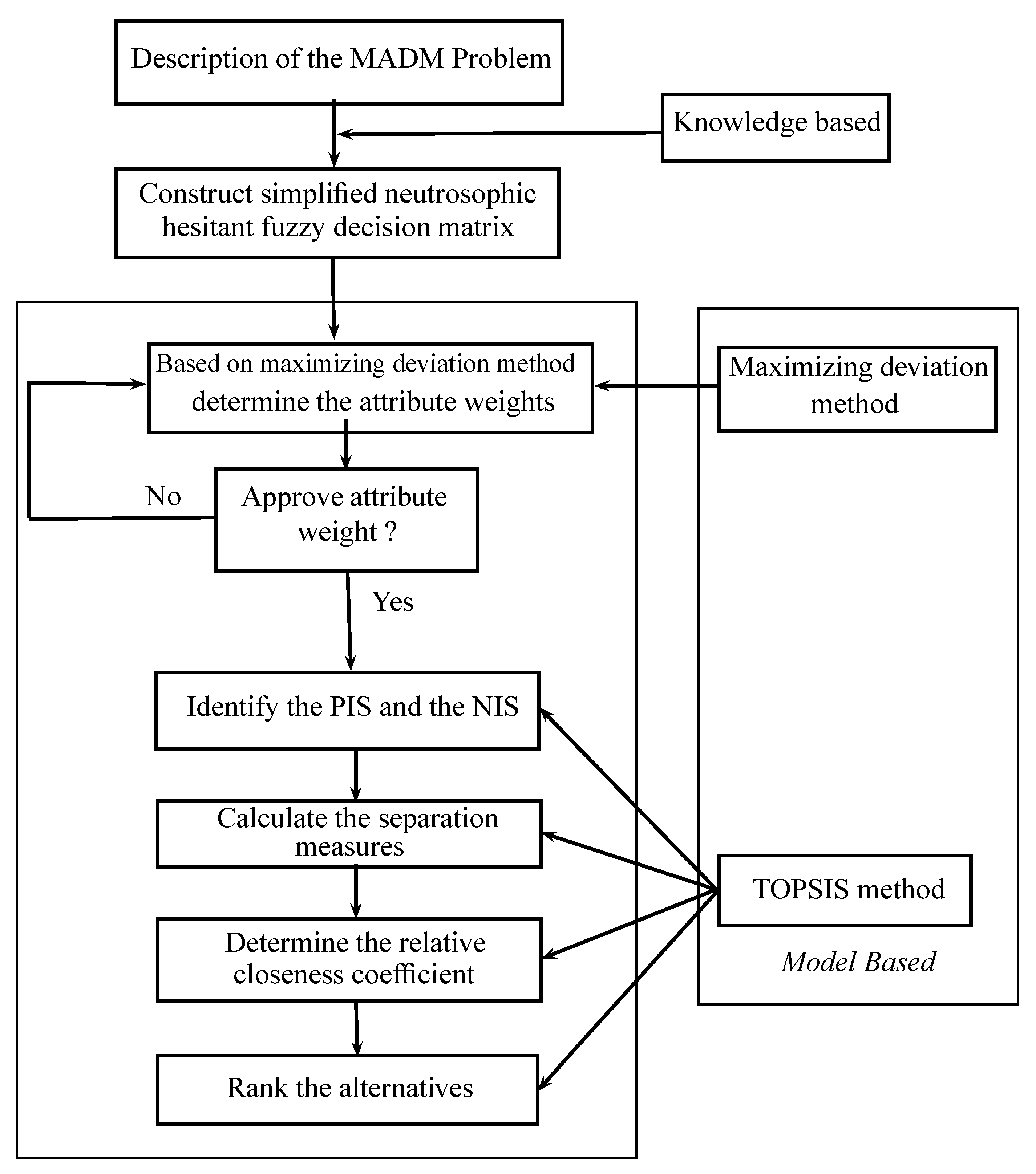
2.1.4. TOPSIS Method
- Step 1.
- Construct the decision matrix for the MADM problem, where the entries are SVNHFEs, given by the decision makers, for the alternative according to the attribute .
- Step 2.
- On the basis of Equation (4) determine the attribute weights , if the attribute weights information is completely unknown, and turn to Step 4. Otherwise go to Step 3.
- Step 3.
- Use model (M-2) to determine the attribute weights , if the information about the attribute weights is partially known.
- Step 4.
- Based on Equations (6) and (8), we determine the corresponding single-valued neutrosophic hesitant fuzzy PIS and the single-valued neutrosophic hesitant fuzzy NIS , respectively.
- Step 5.
- Based on Equations (10) and (12), we compute the separation measures and of each alternative from the single-valued neutrosophic hesitant fuzzy PIS and the single-valued neutrosophic hesitant fuzzy NIS , respectively.
- Step 6.
- Based on Equation (13), we determine the relative closeness coefficient of each alternative to the single-valued neutrosophic hesitant fuzzy PIS .
- Step 7.
- Rank the alternatives based on the relative closeness coefficients and select the optimal one(s).
2.2. TOPSIS and Maximizing Deviation Method for Interval Neutrosophic Hesitant Fuzzy Multi-Attribute Decision-Making
- If , the pessimist expert may add the minimum truth-membership degree , the minimum indeterminacy-membership degree and the minimum falsity-membership degree .
- If , the neutral expert may add the truth-membership degree , the indeterminacy-membership degree and the falsity-membership degree .
- If , the optimistic expert may add the maximum truth-membership degree , the maximum indeterminacy-membership degree and the maximum falsity-membership degree .
| Algorithm 2 The algorithm for the normalization of INHFEs. |
| INPUT: Two INHFEs and and the value of . |
| OUTPUT: The normalization of and . |
| 1: Count the number of elements of and , i.e., , , , , , ; |
| 2: Determine the minimum and the maximum of the elements of and ; |
| 3: , , |
| 4: if then break; |
| 5: else if then |
| 6: ; |
| 7: Determine the value of for ; |
| 8: for i = 1:1:n do |
| 9: ; |
| 10: end for |
| 11: else |
| 12: ; |
| 13: Determine the value of for ; |
| 14: for i = 1:1:n do |
| 15: ; |
| 16: end for |
| 17: end if |
| 18: if then break; |
| 19: else if then |
| 20: ; |
| 21: Determine the value of for ; |
| 22: for i = 1:1:n do |
| 23: ; |
| 24: end for |
| 25: else |
| 26: ; |
| 27: Determine the value of for ; |
| 28: for i = 1:1:n do |
| 29: ; |
| 30: end for |
| 31: end if |
| 32: if then break; |
| 33: else if then |
| 34: ; |
| 35: Determine the value of for ; |
| 36: for i = 1:1:n do |
| 37: ; |
| 38: end for |
| 39: else |
| 40: ; |
| 41: Determine the value of for ; |
| 42: for i = 1:1:n do |
| 43: ; |
| 44: end for |
| 45: end if |
2.2.1. The Distance Measures for INHFSs
- If then the distance .
- If then the distance .
2.2.2. Computation of Optimal Weights Using Maximizing Deviation Method
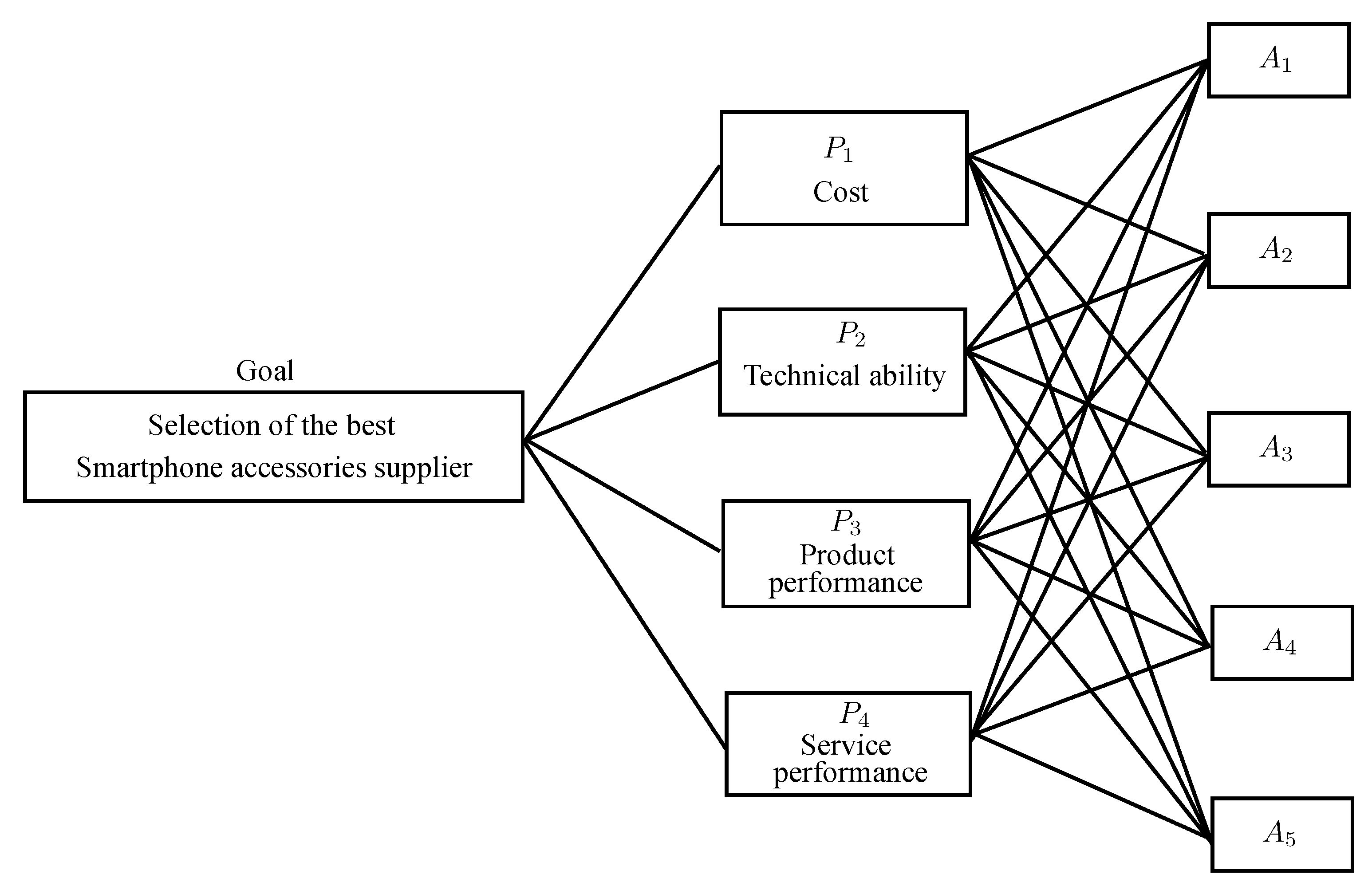
3. An Illustrative Example
- Step 1:
- On the basis of Equation (4), we get the optimal weight vector:
- Step 2:
- Based on the decision matrix of Table 2, we get the normalization of the reference points and as follows:
- Step 3:
- On the basis of Equations (10) and (12), we determine the geometric distances and for the alternative as shown in Table 3.
- Step 4:
- Use Equation (13) to determine the relative closeness of each alternative with respect to the single-valued neutrosophic hesitant fuzzy PIS :
- Step 5:
- On the basis of the relative closeness coefficients , rank the alternatives : . Thus, the optimal alternative (CPU supplier) is .
- Step 1:
- Use the model (M-2) to establish the single-objective programming model as follows:By solving this model, we obtain the attributes weight vector:
- Step 2:
- According to the decision matrix of Table 2, the normalization of the reference points and can be obtained as follows:
- Step 3:
- Based on Equations (10) and (12), we determine the geometric distances and for the alternative as shown in Table 4.
- Step 4:
- Use Equation (13) to determine the relative closeness of each alternative with respect to the single-valued neutrosophic hesitant fuzzy PIS :
- Step 5:
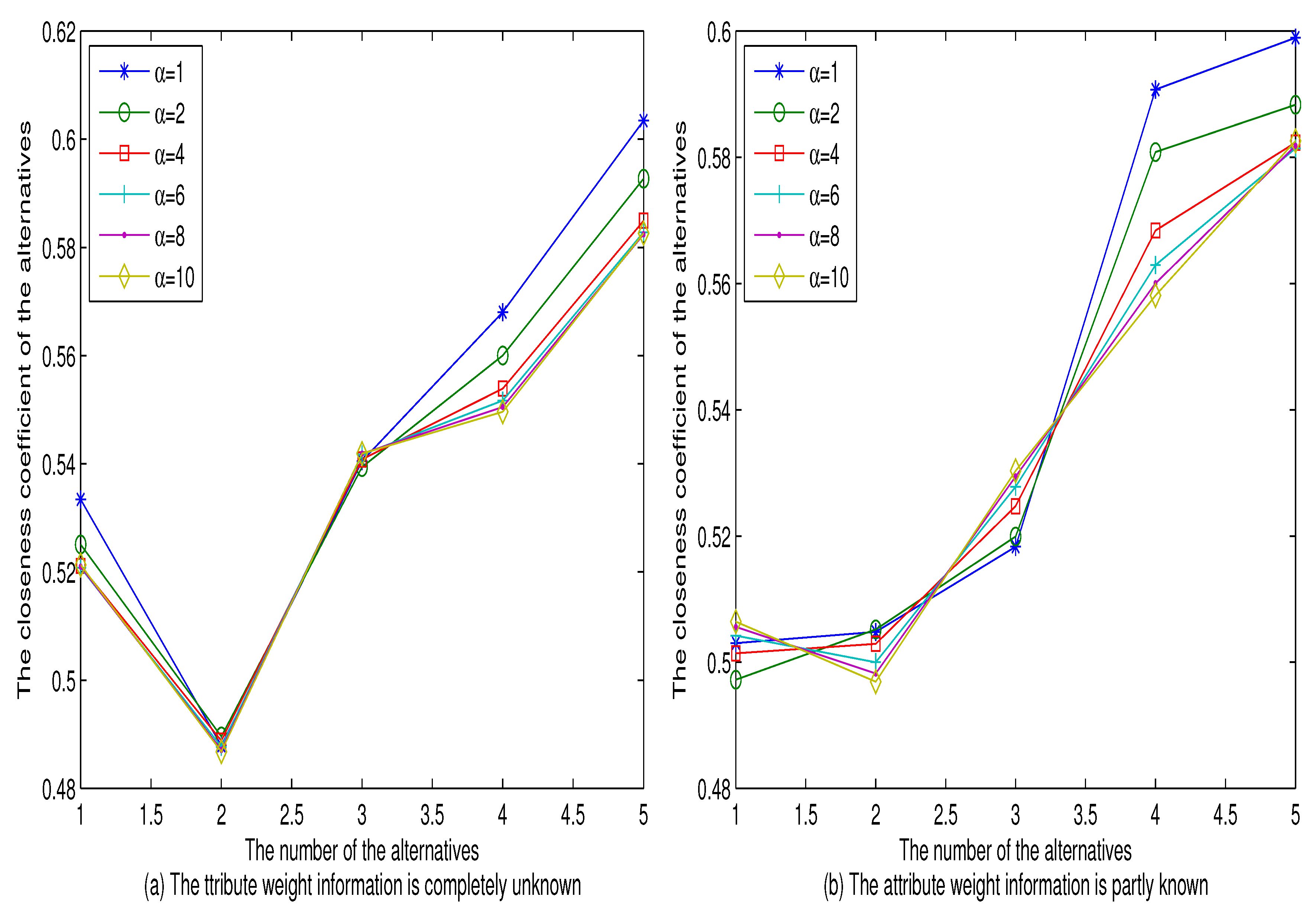
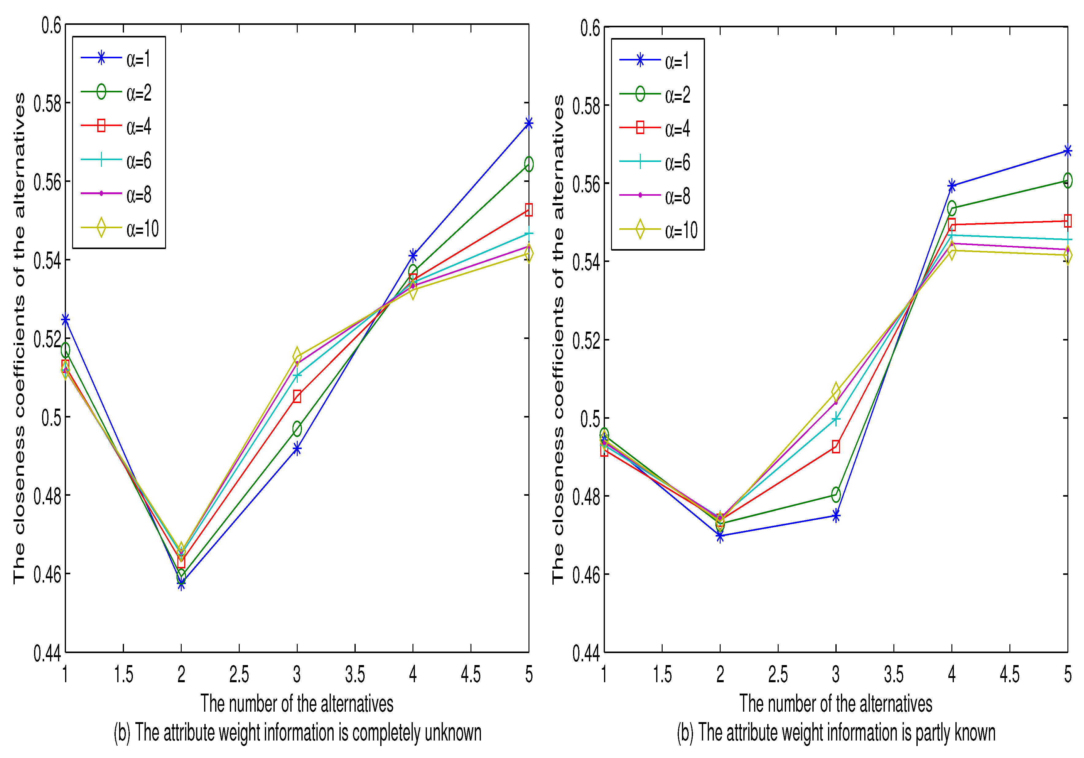
- Based on the relative closeness coefficients , rank the alternatives : . Thus, the optimal alternative (CPU supplier) is .Taking , we normalize the single-valued neutrosophic hesitant fuzzy decision matrix and compute the closeness coefficient of the alternatives with the different values of . The comparison results are given in Figure 3.
- Step 1:
- On the basis of Equation (14), we get the optimal weight vector:
- Step 2:
- According to the decision matrix of Table 6, the normalization of the reference points and can be obtained as follows:
- Step 3:
- Based on Equations (15) and (17), we determine the geometric distances and for the alternative as shown in Table 7.
- Step 4:
- Use Equation (19) to determine the relative closeness of each alternative with respect to the interval neutrosophic hesitant fuzzy PIS :
- Step 5:
- Based on the relative closeness coefficients , rank the alternatives : . Thus, the optimal alternative (CPU supplier) is .
- Step 1:
- Use the model (M-4) to establish the single-objective programming model as follows:By solving this model, we obtain the weight vector of attributes:
- Step 2:
- According to the decision matrix of Table 6, we can obtain the normalization of the reference points and as follows:
- Step 3:
- Use Equations (15) and (17) to determine the geometric distances and for the alternative as shown in Table 8.
- Step 4:
- Use Equation (19) to determine the relative closeness of each alternative with respect to the interval neutrosophic hesitant fuzzy PIS :
- Step 5:
- According to the relative closeness coefficients , rank the alternatives : . Thus, the optimal alternative (CPU supplier) is .
Comparative Analysis
4. Conclusions
Author Contributions
Conflicts of Interest
References
- Smarandache, F. A Unifying Field in Logics. Neutrosophy: Neutrosophic Probability, Set and Logic; American Research Press: Rehoboth, DE, USA, 1999. [Google Scholar]
- Smarandache, F. Neutrosophy. Neutrosophic Probability, Set, and Logic, ProQuest Information & Learning; American Research Press: Ann Arbor, MI, USA, 1998; Volume 105, pp. 118–123. [Google Scholar]
- Wang, H.; Smarandache, F.; Zhang, Y.Q.; Sunderraman, R. Single-valued neutrosophic sets. Multispace Multistruct. 2010, 4, 410–413. [Google Scholar]
- Ye, J. A multi-criteria decision making method using aggregation operators for simplified neutrosophic sets. J. Intell. Fuzzy Syst. 2014, 26, 2459–2466. [Google Scholar]
- Torra, V.; Narukawa, Y. On hesitant fuzzy sets and decision. In Proceedings of the 18th IEEE International Conference on Fuzzy Systems, Jeju Island, Korea, 20–24 August 2009; pp. 1378–1382. [Google Scholar]
- Zadeh, L.A. Fuzzy sets. Inf. Control 1965, 8, 338–353. [Google Scholar] [CrossRef]
- Ye, J. Multiple-attribute decision making method under a single valued neutrosophic hesitant fuzzy environment. J. Intell. Syst. 2015, 24, 23–36. [Google Scholar] [CrossRef]
- Liu, C.F.; Luo, Y.S. New aggregation operators of single-valued neutrosophic hesitant fuzzy set and their application in multi-attribute decision making. Pattern Anal. Appl. 2019, 22, 417–427. [Google Scholar] [CrossRef]
- Sahin, R.; Liu, P. Correlation coefficient of single-valued neutrosophic hesitant fuzzy sets and its applications in decision making. Neural Comput. Appl. 2017, 28, 1387–1395. [Google Scholar] [CrossRef]
- Li, X.; Zhang, X. Single-valued neutrosophic hesitant fuzzy Choquet aggregation operators for multi-attribute decision making. Symmetry 2018, 10, 50. [Google Scholar] [CrossRef]
- Juan-juan, P.; Jian-qiang, W.; Jun-hua, H. Multi-criteria decision making approach based on single-valued neutrosophic hesitant fuzzy geometric weighted choquet integral heronian mean operator. J. Intell. Fuzzy Syst. 2018, 1–14. [Google Scholar] [CrossRef]
- Wang, R.; Li, Y. Generalized single-valued neutrosophic hesitant fuzzy prioritized aggregation operators and their applications to multiple criteria decision making. Information 2018, 9, 10. [Google Scholar] [CrossRef]
- Akram, M.; Adeel, A.; Alcantud, J.C.R. Group decision making methods based on hesitant N-soft sets. Expert Syst. Appl. 2019, 115, 95–105. [Google Scholar] [CrossRef]
- Akram, M.; Adeel, A. TOPSIS approach for MAGDM based on interval-valued hesitant fuzzy N-soft environment. Int. J. Fuzzy Syst. 2019, 21, 993–1009. [Google Scholar] [CrossRef]
- Akram, M.; Adeel, A.; Alcantud, J.C.R. Hesitant Fuzzy N-Soft Sets: A New Model with Applications in Decision-Making. J. Intell. Fuzzy Syst. 2019. [Google Scholar] [CrossRef]
- Akram, M.; Naz, S. A Novel Decision-Making Approach under Complex Pythagorean Fuzzy Environment. Math. Comput. Appl. 2019, 24, 73. [Google Scholar] [CrossRef]
- Naz, S.; Ashraf, S.; Akram, M. A novel approach to decision making with Pythagorean fuzzy information. Mathematics 2018, 6, 95. [Google Scholar] [CrossRef]
- Naz, S.; Ashraf, S.; Karaaslan, F. Energy of a bipolar fuzzy graph and its application in decision making. Italian J. Pure Appl. Math. 2018, 40, 339–352. [Google Scholar]
- Naz, S.; Akram, M. Novel decision making approach based on hesitant fuzzy sets and graph theory. Comput. Appl. Math. 2018. [Google Scholar] [CrossRef]
- Liu, P.; Shi, L. The generalized hybrid weighted average operator based on interval neutrosophic hesitant set and its application to multiple attribute decision making. Neural Comput. Appl. 2015, 26, 457–471. [Google Scholar] [CrossRef]
- Ye, J. Correlation coefficients of interval neutrosophic hesitant fuzzy sets and its application in a multiple attribute decision making method. Informatica 2016, 27, 179–202. [Google Scholar] [CrossRef]
- Kakati, P.; Borkotokey, S.; Mesiar, R.; Rahman, S. Interval neutrosophic hesitant fuzzy Choquet integral in multi-criteria decision making. J. Intell. Fuzzy Syst. 2018, 1–19. [Google Scholar] [CrossRef]
- Mahmood, T.; Ye, J.; Khan, Q. Vector similarity measures for simplified neutrosophic hesitant fuzzy set and their applications. J. Inequal. Spec. Funct. 2016, 7, 176–194. [Google Scholar]
- Atanassov, K.T. Intuitionistic fuzzy sets. Fuzzy Sets Syst. 1986, 20, 87–96. [Google Scholar] [CrossRef]
- Torra, V. Hesitant fuzzy sets. Int. J. Intell. Syst. 2010, 25, 529–539. [Google Scholar] [CrossRef]
- Xu, Z. Some similarity measures of intuitionistic fuzzy sets and their applications to multiple attribute decision making. Fuzzy Optim. Decis. Mak. 2007, 6, 109–121. [Google Scholar] [CrossRef]
- Xu, Z.; Zhang, X. Hesitant fuzzy multi-attribute decision making based on TOPSIS with incomplete weight information. Knowl.-Based Syst. 2013, 52, 53–64. [Google Scholar] [CrossRef]
- Wei, C.; Ren, Z.; Rodriguez, R.M. A hesitant fuzzy linguistic TODIM method based on a score function. Int. J. Comput. Intell. Syst. 2015, 8, 701–712. [Google Scholar] [CrossRef]
- Liao, H.; Xu, Z.; Zeng, X.J. Hesitant fuzzy linguistic VIKOR method and its application in qualitative multiple criteria decision making. IEEE Trans. Fuzzy Syst. 2015, 23, 1343–1355. [Google Scholar] [CrossRef]
- Gou, X.J.; Liao, H.C.; Xu, Z.S.; Herrera, F. Double hierarchy hesitant fuzzy linguistic term set and MULTIMOORA method: A case of study to evaluate the implementation status of haze controlling measures. Inf. Fusion 2017, 38, 22–34. [Google Scholar] [CrossRef]
- Zhao, H.; Xu, Z.; Wang, H.; Liu, S. Hesitant fuzzy multi-attribute decision making based on the minimum deviation method. Soft Comput. 2017, 21, 3439–3459. [Google Scholar] [CrossRef]


| {{0.2},{0.3,0.5},{0.1,0.2,0.3}} | {{0.6,0.7},{0.1,0.3},{0.2,0.4}} | |
| {{0.1},{0.3},{0.5,0.6}} | {{0.4},{0.3,0.5},{0.5,0.6}} | |
| {{0.6,0.7},{0.2,0.3},{0.1,0.2}} | {{0.1,0.2},{0.3},{0.6,0.7}} | |
| {{0.2,0.3},{0.1,0.2},{0.5,0.6}} | {{0.3,0.4},{0.2,0.3},{0.5,0.6,0.7}} | |
| {{0.7},{0.4,0.5},{0.2,0.4,0.5}} | {{0.6},{0.1,0.7},{0.3,0.5}} | |
| {{0.2,0.3},{0.4},{0.7,0.8}} | {{0.4},{0.1,0.3},{0.5,0.7,0.9}} | |
| {{0.1,0.3},{0.4},{0.5,0.6,0.8}} | {{0.6,0.8},{0.2},{0.3,0.5}} | |
| {{0.2,0.3},{0.1,0.2},{0.6,0.7}} | {{0.2,0.3},{0.4},{0.2,0.5,0.6}} | |
| {{0.2,0.4},{0.3},{0.1,0.2}} | {{0.6},{0.2},{0.3,0.5}} | |
| {{0.3},{0.5},{0.1,0.4}} | {{0.5},{0.1,0.2},{0.3,0.4}} |
| {{0.2,0.2},{0.3,0.5},{0.1,0.2,0.3}} | {{0.6,0.7},{0.1,0.3},{0.2,0.3,0.4}} | |
| {{0.1,0.1},{0.3,0.3},{0.5,0.55,0.6}} | {{0.4,0.4},{0.3,0.5},{0.5,0.55,0.6}} | |
| {{0.6,0.7},{0.2,0.3},{0.1,0.15,0.2}} | {{0.1,0.2},{0.3,0.3},{0.6,0.65,0.7}} | |
| {{0.2,0.3},{0.1,0.2},{0.5,0.55,0.6}} | {{0.3,0.4},{0.2,0.3},{0.5,0.6,0.7}} | |
| {{0.7,0.7},{0.4,0.5},{0.2,0.4,0.5}} | {{0.6,0.6},{0.1,0.7},{0.3,0.4,0.5}} | |
| {{0.2,0.3},{0.4,0.4},{0.7,0.75,0.8}} | {{0.4,0.4},{0.1,0.3},{0.5,0.7,0.9}} | |
| {{0.1,0.3},{0.4,0.4},{0.5,0.6,0.8}} | {{0.6,0.8},{0.2,0.2},{0.3,0.4,0.5}} | |
| {{0.2,0.3},{0.1,0.2},{0.6,0.65,0.7}} | {{0.2,0.3},{0.4,0.4},{0.2,0.5,0.6}} | |
| {{0.2,0.4},{0.3,0.3},{0.1,0.15,0.2}} | {{0.6,0.6},{0.2,0.2},{0.3,0.4,0.5}} | |
| {{0.3,0.3},{0.5,0.5},{0.1,0.25,0.4}} | {{0.5,0.5},{0.1,0.2},{0.3,0.35,0.4}} |
| Geometric Distance | |||||
|---|---|---|---|---|---|
| 0.5142 | 0.5434 | 0.4974 | 0.4781 | 0.4279 | |
| 0.5685 | 0.5212 | 0.5824 | 0.6086 | 0.6226 |
| Geometric Distance | |||||
|---|---|---|---|---|---|
| 0.5446 | 0.5244 | 0.5220 | 0.4534 | 0.4341 | |
| 0.5385 | 0.5355 | 0.5652 | 0.6281 | 0.6202 |
| {{[0.2,0.3]},{[0.3,0.4],[0.5,0.7]},{[0.1,0.3],[0.2,0.5],[0.3,0.6]}} | {{[0.6,0.8],[0.7,0.9]},{[0.1,0.2],[0.3,0.5]},{[0.2,0.3],[0.4,0.5]}} | |
| {{[0.1,0.3]},{[0.3,0.5]},{[0.5,0.7],[0.6,0.8]}} | {{[0.4,0.6]},{[0.3,0.4],[0.5,0.6]},{[0.5,0.7],[0.6,0.8]}} | |
| {{[0.6,0.7],[0.7,0.8]},{[0.2,0.4],[0.3,0.5]},{[0.1,0.3],[0.2,0.4]}} | {{[0.1,0.3],[0.2,0.4]},{[0.3,0.6]},{[0.6,0.8],[0.7,0.9]}} | |
| {{[0.2,0.5],[0.3,0.4]},{[0.1,0.3],[0.2,0.3]},{[0.5,0.6],[0.6,0.7]}} | {{[0.3,0.5],[0.4,0.6]},{[0.2,0.3],[0.3,0.4]},{[0.5,0.7],[0.6,0.8],[0.7,0.9]}} | |
| {{[0.7,0.8]},{[0.4,0.6],[0.5,0.7]},{[0.2,0.3],[0.4,0.6],[0.5,0.7]}} | {{[0.6,0.8]},{[0.1,0.3],[0.7,0.8]},{[0.3,0.4],[0.5,0.6}} | |
| {{[0.2,0.4],[0.3,0.5]},{[0.4,0.5]},{[0.7,0.8],[0.8,0.9]}} | {{[0.4,0.6]},{[0.1,0.2],[0.3,0.4]},{[0.5,0.6],[0.7,0.8],[0.8,0.9]}} | |
| {{[0.1,0.3],[0.3,0.5]},{[0.4,0.6]},{[0.5,0.6],[0.6,0.7],[0.8,0.9]}} | {{[0.6,0.7],[0.8,0.9]},{[0.2,0.5]},{[0.3,0.5],[0.5,0.7]}} | |
| {{[0.2,0.3],[0.3,0.4]},{[0.1,0.3],[0.2,0.4]},{[0.6,0.8],[0.7,0.9]}} | {{[0.2,0.4],[0.3,0.5]},{[0.4,0.6]},{[0.2,0.3],[0.5,0.7],[0.6,0.8]}} | |
| {{[0.2,0.3],[0.4,0.5]},{[0.3,0.6]},{[0.1,0.4],[0.2,0.5]}} | {{[0.6,0.8]},{[0.2,0.3]},{[0.3,0.4],[0.5,0.6]}} | |
| {{[0.3,0.5]},{[0.5,0.6]},{[0.1,0.3],[0.4,0.5]}} | {{[0.5,0.7]},{[0.1,0.3],[0.2,0.5]},{[0.3,0.5],[0.4,0.8]}} |
| {{[0.2,0.3],[0.2,0.3]},{[0.3,0.4],[0.5,0.7]},{[0.1,0.3],[0.2,0.5],[0.3,0.6]}} | {{[0.6,0.8],[0.7,0.9]},{[0.1,0.2],[0.3,0.5]},{[0.2,0.3],[0.3,0.4],[0.4,0.5]}} | |
| {{[0.1,0.3],[0.1,0.3]},{[0.3,0.5],[0.3,0.5]},{[0.5,0.7],[0.55,0.75],[0.6,0.8]}} | {{[0.4,0.6],[0.4,0.6]},{[0.3,0.4],[0.5,0.6]},{[0.5,0.7],[0.55,0.75],[0.6,0.8]}} | |
| {{[0.6,0.7],[0.7,0.8]},{[0.2,0.4],[0.3,0.5]},{[0.1,0.3],[0.15,0.35],[0.2,0.4]}} | {{[0.1,0.3],[0.2,0.4]},{[0.3,0.6],[0.3,0.6]},{[0.6,0.8],[0.65,0.85],[0.7,0.9]}} | |
| {{[0.2,0.5],[0.3,0.4]},{[0.1,0.3],[0.2,0.3]},{[0.5,0.6],[0.55,0.65],[0.6,0.7]}} | {{[0.3,0.5],[0.4,0.6]},{[0.2,0.3],[0.3,0.4]},{[0.5,0.7],[0.6,0.8],[0.7,0.9]}} | |
| {{[0.7,0.8],[0.7,0.8]},{[0.4,0.6],[0.5,0.7]},{[0.2,0.3],[0.4,0.6],[0.5,0.7]}} | {{[0.6,0.8],[0.6,0.8]},{[0.1,0.3],[0.7,0.8]},{[0.3,0.4],[0.4,0.5],[0.5,0.6}} | |
| {{[0.2,0.4],[0.3,0.5]},{[0.4,0.5],[0.4,0.5]},{[0.7,0.8],[0.75,0.85],[0.8,0.9]}} | {{[0.4,0.6],[0.4,0.6]},{[0.1,0.2],[0.3,0.4]},{[0.5,0.6],[0.7,0.8],[0.8,0.9]}} | |
| {{[0.1,0.3],[0.3,0.5]},{[0.4,0.6],[0.4,0.6]},{[0.5,0.6],[0.6,0.7],[0.8,0.9]}} | {{[0.6,0.7],[0.8,0.9]},{[0.2,0.5],[0.2,0.5]},{[0.3,0.5],[0.4,0.6],[0.5,0.7]}} | |
| {{[0.2,0.3],[0.3,0.4]},{[0.1,0.3],[0.2,0.4]},{[0.6,0.8],[0.65,0.85],[0.7,0.9]}} | {{[0.2,0.4],[0.3,0.5]},{[0.4,0.6],[0.4,0.6]},{[0.2,0.3],[0.5,0.7],[0.6,0.8]}} | |
| {{[0.2,0.3],[0.4,0.5]},{[0.3,0.6],[0.3,0.6]},{[0.1,0.4],[0.15,0.45],[0.2,0.5]}} | {{[0.6,0.8],[0.6,0.8]},{[0.2,0.3],[0.2,0.3]},{[0.3,0.4],[0.4,0.5],[0.5,0.6]}} | |
| {{[0.3,0.5],[0.3,0.5]},{[0.5,0.6],[0.5,0.6]},{[0.1,0.3],[0.25,0.4],[0.4,0.5]}} | {{[0.5,0.7],[0.5,0.7]},{[0.1,0.3],[0.2,0.5]},{[0.3,0.5],[0.35,0.65],[0.4,0.8]}} |
| Geometric Distance | |||||
|---|---|---|---|---|---|
| 0.5169 | 0.5711 | 0.5361 | 0.4952 | 0.4625 | |
| 0.5531 | 0.4849 | 0.5295 | 0.5740 | 0.5991 |
| Geometric Distance | |||||
|---|---|---|---|---|---|
| 0.5406 | 0.5562 | 0.5569 | 0.4752 | 0.4653 | |
| 0.5310 | 0.4990 | 0.5147 | 0.5894 | 0.5938 |
| Methods | Score of Alternatives | Ranking of Alternatives |
|---|---|---|
| Zhao et al. [31] for SVNHFS | 0.4431 0.4025 0.4941 0.5073 0.5691 | |
| Our proposed method for SVNHFS | 0.5251 0.4896 0.5394 0.5600 0.5927 | |
| Zhao et al. [31] for INHFS | 0.4559 0.4206 0.4255 0.5334 0.5791 | |
| Our proposed method for INHFS | 0.5169 0.4592 0.4969 0.5368 0.5643 |
© 2019 by the authors. Licensee MDPI, Basel, Switzerland. This article is an open access article distributed under the terms and conditions of the Creative Commons Attribution (CC BY) license (http://creativecommons.org/licenses/by/4.0/).
Share and Cite
Akram, M.; Naz, S.; Smarandache, F. Generalization of Maximizing Deviation and TOPSIS Method for MADM in Simplified Neutrosophic Hesitant Fuzzy Environment. Symmetry 2019, 11, 1058. https://doi.org/10.3390/sym11081058
Akram M, Naz S, Smarandache F. Generalization of Maximizing Deviation and TOPSIS Method for MADM in Simplified Neutrosophic Hesitant Fuzzy Environment. Symmetry. 2019; 11(8):1058. https://doi.org/10.3390/sym11081058
Chicago/Turabian StyleAkram, Muhammad, Sumera Naz, and Florentin Smarandache. 2019. "Generalization of Maximizing Deviation and TOPSIS Method for MADM in Simplified Neutrosophic Hesitant Fuzzy Environment" Symmetry 11, no. 8: 1058. https://doi.org/10.3390/sym11081058
APA StyleAkram, M., Naz, S., & Smarandache, F. (2019). Generalization of Maximizing Deviation and TOPSIS Method for MADM in Simplified Neutrosophic Hesitant Fuzzy Environment. Symmetry, 11(8), 1058. https://doi.org/10.3390/sym11081058