Abstract
Fine-grained image classification is a challenging problem because of its large intra-class differences and low inter-class variance. Bilinear pooling based models have been shown to be effective at fine-grained classification, while most previous approaches neglect the fact that distinctive features or modeling distinguishing regions usually have an important role in solving the fine-grained problem. In this paper, we propose a novel convolutional neural network framework, i.e., attention bilinear pooling, for fine-grained classification with attention. This framework can learn the distinctive feature information from the channel or spatial attention. Specifically, the channel and spatial attention allows the network to better focus on where the key targets are in the image. This paper embeds spatial attention and channel attention in the underlying network architecture to better represent image features. To further explore the differences between channels and spatial attention, we propose channel attention bilinear pooling (CAB), spatial attention bilinear pooling (SAB), channel spatial attention bilinear pooling (CSAB), and spatial channel attention bilinear pooling (SCAB) as four alternative frames. A variety of experiments on several datasets show that our proposed method has a very impressive performance compared to other methods based on bilinear pooling.
1. Introduction
As an important branch of artificial intelligence, computer vision deals with how computers can be made to gain a high-level understanding from digital images or videos, so as to complete object recognition [1,2,3], detection [4,5], classification [6,7], and other vision-related tasks. According to the fineness of classification, image classification can be divided into coarse-grained image classification and fine-grained image classification [8]. The classification of coarse-grained images differs greatly from each other, and there is no obvious subordinate relationship between the categories and it is easy to distinguish the different categories, however, the gap between fine-grained image classes is small, and the classification categories generally belong to different sub-categories under the same parent class.
Fine-grained image classification aims at distinguishing finer subclasses from the base category, which is a challenging research topic in the field of computer vision within the development of science and technology. Different from the coarse-grained classification, fine-grained image classification is more difficult for the following reasons. Firstly, different subcategories share similar structures and differ in subtle local areas, which leads to low inter-class variance (e.g., the three pictures in Figure 1b–d respectively belong to Brewer Blackbird, Shiny Cowbird, and Rusty Blackbird with little differences in Figure 1). High intra-class variance also exists due to uncertain factors such as attitude, illumination, occlusion, background interference (e.g., the three pictures in Figure 1a all belong to Black-Footed Albatross with great differences). Secondly, subcategories are numerous while training data are limited. Third, specific domain expertise and a certain information reserve are required in data collection and annotation. Samples of CUB-200-2011 [9] are shown in Figure 1.
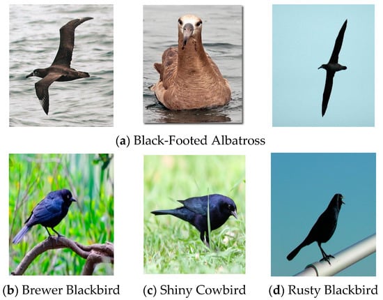
Figure 1.
Challenges in fine-grained image classification: (a) There is a large variation in the same subclass; (b–d) there is little in variation between different subclasses.
There has been a lot of research into fine-grained classification. Motivated by the observation of the importance of the local parts of an object in order to differentiate between subcategories, many methods [10,11,12,13,14,15,16,17,18] for fine-grained classification were developed by exploiting the difference between local parts. According to the methods of modeling local regions, the current fine-grained algorithms can be roughly divided into two methods. The first method is the strong supervised learning method [10,11,12] by manual annotation, which localizes different parts of an object by utilizing available bounding boxes or part annotations and then extracts the discriminative features for classification. However, approaches that rely on prior knowledge suffer from two essential limitations. First, it is difficult to ensure the manually defined parts are optimal or suitable for the fine-grained classification task. Second, detailed part annotations are likely to be time-consuming and labor-intensive, which is not feasible in practice. The other method is the deep learning method [13,14,15,16,17,18] which employs the convolutional neural network (CNN) to detect local parts and extract features, then merge local and global regional features to get the high-level semantic features of the original image and better characterize features. In this way, local features are extracted, and research in this area has progressed considerably. Unlike the above methods, we focus on the channel and spatial dimensions of the feature map, treating activations from different channels and spatial locations as responses to different component properties, rather than explicitly locating the objects’ components by adding different channels, and the spatial dimension attention information with bilinear pooling modeling the local characteristics. Moreover, we verify the effectiveness of the proposed method on three different fine-grained datasets CUB-200-2011, Stanford cars [19], and FGVC-aircraft [20].
Alternatively, various research has [13,14,15,16,17,18] utilized bilinear pooling frameworks to model local parts of the object. For example, Lin et al. [13] proposed the bilinear pooling framework to localize parts of the object and then [14,15,16,17,18] have achieved certain progress based on it. However, they all have certain limitations, such as directly taking the features of the last convolutional layer as feature representations, neglecting the different roles of each channel and each spatial position of the feature map in the classification result, instead of an accurate description of image features.
To solve the problem, we propose a novel attention bilinear pooling framework. Paper [21] indicates that each channel convolution layer in the classification of contribution is different and so is the spatial cell. In order to better describe the image features, we put forward a bilinear pooling attention model, which adopts the attention mechanism to tap the image characteristics of different dimensions for accurately modeling the local features. The attention mechanism can learn to get the weight of channel or cell, and further, to know the discriminant region, then assign a considerable weight to the discriminant local area to enhance the feature expression ability and discriminant ability of the model, which is more useful for the classification task. At the same time, we explored the channel attention, spatial attention, different channel spatial attention, and spatial attention double bilinear pooling method to study the difference between channel and spatial detection for classification results. This method is proved to be useful for fine-grained feature learning. The theoretical framework we proposed is in Figure 2 as follows.
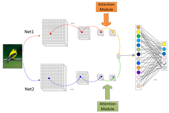
Figure 2.
The structure of attention bilinear pooling.
The contributions of this paper are as follows:
Firstly, we propose a simple but effective attention bilinear pooling theory, which can make full use of the channel and spatial feature information to model distinctive features and represent the local information of the image in a simple and effective way. Secondly, our attention model adopts the superposition mode, which not only considers the attention information but also retains the original channel information. This simple superposition mode enables the module to be directly transferred to other frameworks. Finally, we conducted comprehensive experiments on three changing datasets (CUB-200-2011, Stanford cars, and FGVC-aircraft), and the results show the effectiveness of our proposed theory.
2. Related Work
In this section, we briefly review related works from two viewpoints of interest, including fine-grained feature extraction and the attention mechanism. The performance of any biometric recognition system heavily depends on finding a suitable feature-representation space where observations from different classes are well separated [22]. In this paper, we obtain the desired fine-grained feature representation space through the fine-grained feature extraction and attention mechanism.
2.1. Fine-Grained Feature Extraction
Feature extracting plays a significant and fundamental role in fine-grained classification. The differences between the fine-grained subclasses are subtle and local, and the global semantic information that limits the output of the last convolutional layer, only with fully connected layers, which, like general image classification, does not represent the image features well. Lin et al. proposed a bilinear structure (BCNN), which extracts the second-order information of the image, and more discriminatively than the convolution features extracted directly. The model consists of two parallel feature extractors with AlexNet [23] or VGGNet [24] removing the final fully connected layer and softmax layer acting as a feature extraction to extract the image. After extracting the corresponding features of each position respectively, the cross product of the feature vectors is taken to obtain the bilinear features of each position. Then, the global bilinear features can be obtained by pooling the features at different locations, and then the normalization and dimensionality reduction operations can be used for classification. Bilinear CNN is one of the first models for “end-to-end” training in the fine-grained classification field, which greatly improves the accuracy of classification. Afterwards, in order to reduce the dimension of linear features and reduce memory consumption, and to simultaneously accelerate the training and recognition speed, Gao et al. employed two mapping methods, random Maclaurin [25] (RM) and tensor sketch [26] (TS), to reduce the feature dimension [14]. Cui et al. proposed the nuclear pooling (Kernel pooling) method to extract the image of the higher-order information [15], which obtained a multi-order feature representation of the image by concatenating different order information. Reference [16] used a low-rank approximation to simplify bilinear confluence. Li et al. completed the image classification task by making a low-rank approximation of the parameter matrix [17], which also contains first-order information. Reference [18] captured the characteristics of higher-order interactions, and the parameters are at rank one approximation. However, these methods only use the convolution feature of a single layer and cannot fully represent the features of an object. The method proposed in this paper can further increase the attention for the discrimination region by modeling the local region through the attention mechanism and effectively solve these problems. In addition, reference [22] compares and analyses the existing feature representation technologies, which can provide some reference for fine-grained feature extraction.
2.2. Attention Mechanism
With the development of deep learning, convolutional neural networks have become a typical feature extractor. The features extracted directly by a single convolutional layer cannot fully represent the features of fine-grained images, so some studies try to explore the convolution features obtained in CNN through the attention mechanism to represent the features better. The attention mechanism is similar to the visual attention of human beings. First, it rapidly scans the global image to locate the target area that needs to be focused. Then, it pays more attention to these areas to collect more detailed information about the target so as to suppress other useless information.
The attention mechanism primarily consists of two parts: Firstly, to determine the area that needs to be paid attention to; secondly, to extract features from essential parts to obtain necessary information. Fu et al. designed the recurrent neural network (RACNN), which circulatively conducted the local region localization and fine-grained feature learning to promote each other [27]. RACNN consists of a classification subnetwork and a visual attention subnetwork. Based on the previous prediction, the visual attention subnetwork gradually narrowed the visible attention area from the original image, and then inputs this area into the classification subnetwork through the pairing rank loss, forcing the visible attention area to gradually shrink while improving the accuracy of the classification prediction. In this way, the algorithm can increasingly focus on the most distinct region, remove the influence of the background environment, and improve the effect of object feature extraction. The MACNN [28] model can focus on multiple local areas at a time. The algorithm moves the visual attention area to the most different part of the image through training, extracts the corresponding features, and fuses the final features to classify. In reference [29,30,31], the learned attention weight is directly applied to the original image. SENet [21] explored the relationship between the different characteristics of the channel, learning to automatically detect the importance of the characteristics of each channel, and then according to the importance to enhance useful features and suppress useless ones adaptively to realign the channel response characteristics. In addition, reference [32] shows that different object locations (convolution kernels) contribute differently to image classification. Woo et al. [33] applies attention to the three different dimensions of scale, feature channel, and space at the same time, and improves the feature extraction ability of the network model while not significantly increasing the amount of computation and parameters. Inspired by [33], we propose the bilinear pooling model of attention.
3. Attention Bilinear Model
The key to fine-grained image classification is to find subtle differences in local areas. In this paper, the attention bilinear pooling model is used to model local regions and increase the weight of the distinguishing regions, so as to enhance the useful features and suppress the useless ones to achieve simple but useful feature representation. In this section, we first give an overview of the whole pipeline and then introduce it in detail by dividing it into two modules.
3.1. The Overall Framework
As illustrated in Figure 3, the attention bilinear model consists of two modules: A feature extractor and an attention bilinear pooling model. In the first module, we extract features by Net1 and Net2, which we all choose VGG-16 [24] for its high performance.
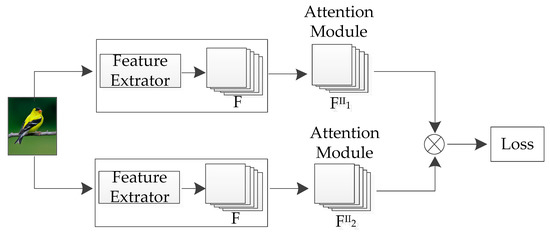
Figure 3.
The overall Framework. F(x) represents image feature, FII1, and FII2 represent features obtained through different attention mechanisms.
In the first module, the extractor starts with a generic classification network to work as a feature extractor for the whole image, and the extracted features are indistinguishable, that is to say, all the features have the same effect on classification. As we all know, underlying image features focus on information such as image edges, and the middle features focus on patterns to learn more complex shapes and other information, while the width and height of deeper feature maps are rich in semantic features due to multi-layer pooling and convolution for image content and other information, so we take the last convolutional layer output feature map conv5_3 as the initial feature representation.
In the second module, the attention mechanism is embedded into the network, and the features obtained in the first module are analyzed and combined in different dimensions so that the network pays attention to the features that are more effective for classification to obtain the optimal feature representation and finally to classify.
3.2. Feature Extractor
The VGG convolutional neural network is a model proposed by Oxford University in 2014. It shows excellent results in both image classification and target detection tasks. Here we use VGG-16 as our feature extractor.
Given an image X, we extract convolutional features F(x) by feeding images into convolutional networks. Using W to denote all parameters, and ∗ to denote a set of operations of convolution, activation, and pooling, extracted image feature F is written as:
3.3. Attention Module
The convolutional features obtained by VGG-16 are not discriminative. Therefore, we introduce the attention mechanism to improve the resolution of features, before discussing the attention mechanism, we first introduce different dimensions of the feature map.
3.3.1. Different Dimensions of the Feature Map
The feature map is the result of convolution and pooling of the input image or convolutional layer through the neural network. The relationship between multiple feature channels has two dimensions [33], which is shown in Figure 4. One is the channel dimension, that is, in the feature channel unit, the relationship between the feature channels is concerned, for example, by grouping the feature channels to acquire the features of different components. The other is the spatial dimension, which is a unit of cell state on the feature channel, focusing on the relationship between points on a feature channel.
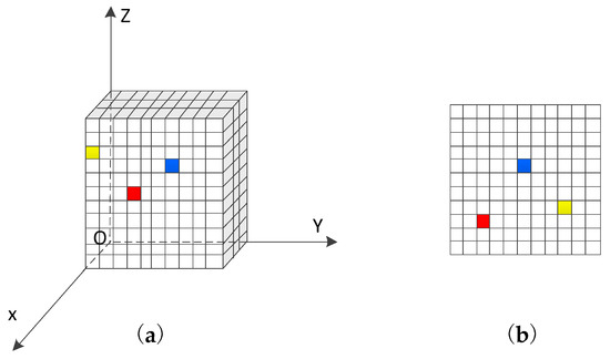
Figure 4.
Different aspects of the feature map: (a) the shape of the feature map; (b) a channel parallel to the YOZ plane.
As shown in Figure 4, Figure 4a mainly shows the shape of the feature map, while Figure 4b is the feature channel parallel to the YOZ plane, the X-axis is in the direction of the feature dimension, and the point on the feature channel is the spatial position. The cell relationship is the spatial dimension.
The attention mechanism of this paper is mainly applied to the channel and spatial dimensions, so the attention module is divided into a channel attention module and spatial attention module.
3.3.2. Channel Attention Module
Different channels can be seen as the response of various components to the convolution kernel. Many studies now treat the effects of different channels on the final result to be equal. For example, Wei et al. simply added the feature maps of the convolution output which made the generated saliency map disturbed by the background of the cluttered image, but the contribution of different channels to the classification is different [34].
In order to highlight the significant region while suppressing the rest of the noise interference, we use the channel attention mechanism to obtain a more discriminative area for fine-grained target location, then increase its weight, and reduce the noise response map weight to suppress invalid channel information and enhance useful channel information.
The primary function of the channel attention is to learn the weight according to the importance of different channels and then weight it to the channel to achieve the effect of strengthening the effective channel information and suppressing the invalid channel information. Global average pooling (GAP) can make full use of the spatial information of the channel but does not have the various parameters of the fully connected layer, which is robust and not easy to be over-fitting. Global max pooling (GMP) can reflect the global maximum response and indicate the critical information in the channel to a certain extent, which can complement the GAP. Therefore, here we use both the GAP and GMP information fusion method to train the learning channel weights.
In addition, as we all know, the role of the convolution kernel is extracting features. The larger the convolution kernel size, the larger the receptive field, the more the parameters. The 1 × 1 convolution first appeared in [35] and was further applied in [36,37]. The original picture or channel can be transformed to get a new one through a 1 × 1 convolution, which can improve the generalization ability and reduce over-fitting. Simultaneously, according to the selected number of 1 × 1 convolutions and filters, cross-channel interaction and information integration can be realized, and the dimensions of the pictures can be changed because there is a significant reduction of operations to aspects of the network parameters, and the calculation amount is saved. Therefore, 1 × 1 convolution is applied to the channels obtained by GAP and GMP in our method, which realizes the interaction of channel information, and dramatically reduces the amount of data compared with the full connection layer.
For the last convolutional layer of the VGG-16, the GAP and GMP compression feature dimensions are first used to obtain the attention maps and . The convolutional block attention module (CBAM) [33] shows that the global average pooling and global maximum pooling information fusion is more effective than using only one pooling method alone. For a deep convolutional neural network, the last layer of the convolutional layer contains the most sufficient spatial and semantic information after multiple convolutions and pooling, which is the optimal representation. The feature map that was last obtained during the convolution phase is the result of multiple previous convolutions, activations, and pooling, with the most robust spatial and semantic information. Therefore, here, we use the attention mechanism after the feature map of the last convolutional layer output. Unlike CBAM, our method only applies the attention module to the last convolutional layer. The initial channel attention is shown in Figure 4.
Figure 5 shows the initial channel attention frame. The input feature map gets and with GAP and GMP respectively, then connects two layers of 1 × 1 convolution to realize the change of channel dimension, realizing cross-dimensional interaction and information fusion, where the number of intermediate feature channels is set to . The effect of the value of on the classification results is detailed in Section 4.2.1. The middle feature channel uses the ReLu activation function which turns the linearity of the convolution into nonlinearity, adds more nonlinear factors, learns more features, and dramatically increases the nonlinear characteristics under the premise of keeping the feature map size unchanged. After the two layers of 1 × 1 convolution, the and are merged and passed to the sigmoid activation function. The activation function limits the weight from 0 to 1, then the resulting normalized weight map represents the importance of each feature channel, which is then weighted by multiplication to the initial channel F, and the re-calibration of the original features in the spatial dimension is completed, meaning the weight distribution is performed on each feature channel in 512 × 28 × 28 to suppress useless information and increase the proportion of useful information. The resulting initial channel attention is:
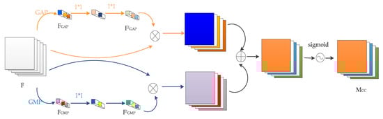
Figure 5.
The initial channel attention of our method, without a depiction of the ReLu function.
Since part of the channel information is lost during information transfer by GAP and GMP, inspired by the residual learning of ResNet [35], the direct connection channel is added to the attention module, and the input of the feature map is directly bypassed to the output to protect the integrity of the information. At the same time, the network only needs to learn the attention module while not needing to learn the entire output. Finally, the convolution feature of the attention module and the original output is superimposed to achieve optimal representation. The resulting feature channel makes a differentiated selection of feature information and combines the feature channel information in this way. The attention module frame diagram is shown in Figure 6.
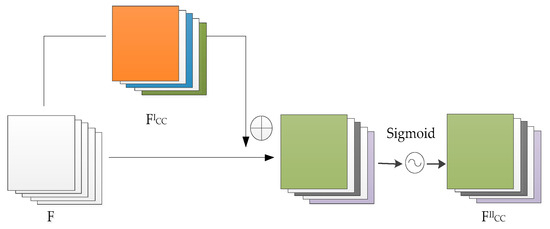
Figure 6.
Channel Attention module.
The channel attention is added as a side branch to the initial feature channel, and final output feature map is:
where represents the sigmoid function, represents pixel-by-pixel addition and represents element-by-element multiplication.
3.3.3. Spatial Attention Module
Channel attention focuses on what makes sense in the input picture, while spatial attention focuses on location information. Different pixels of the same channel are also of varying importance to the classification results. The role of the spatial attention module is to assign more weight to key parts and increase the focus on the objects in the diagram. The spatial attention can be understood to assign a weight value for each pixel of the feature map to enhance the crucial area and weaken the invalid area. The spatial attention module frame diagram is shown in Figure 7.
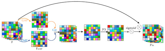
Figure 7.
Initial spatial attention.
In the same way as the channel attention module, first, we adopt the GAP and GMP to get and , note that the GAP and GMP are all along the channel dimension. Then and are converted to a 3 × 3 convolution layer, and sigmoid function is used to obtain the attention map . Finally, the attention map is multiplied by the pixel and the initial feature map to get the initial spatial attention module .
Similarly, we adopt the direct connection channel and get the final spatial attention module after adding the initial feature channel, which is shown in Figure 8.
where represents the sigmoid function, f represents 3 × 3 convolution operation and represents element-by-element multiplication.
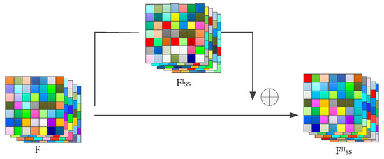
Figure 8.
Spatial attention module.
3.3.4. Double Attention Module
Channel attention and spatial attention resolve image features in two different dimensions, so embedding channel and spatial attention simultaneously facilitates convolutional neural networks to learn more feature information, which not only helps to focus on what the object is but also contributes to paying attention to the position information of the object, and the two dimensions complement and promote each other. Therefore, here we use the dual attention model to get the attention of two different dimensions of channel and space. Figure 9 shows a double attention frame.
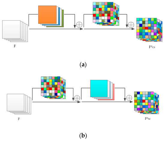
Figure 9.
Double attention module. (a) Channel spatial attention module. (b) Spatial channel attention module.
Figure 9a shows a frame diagram of embedding channel attention and then adding spatial attention, while Figure 9b shows a frame diagram of adding spatial attention and then adding channel attention. The effect of the sequence of attention on the results is discussed in detail in Section 4.2.3.
In Figure 9a we firstly adopt the channel attention to get , and then add the spatial attention. Similar to Section 3.3, and are obtained through GAP and GMP, and the resulting double attention module is:
In Figure 9b, firstly, we adopt spatial attention to get , then add channel attention, and the resulting double attention module is:
3.3.5. Bilinear Pooling
We still used the bilinear pooling model proposed in BCNN. Lin et al. proposed the bilinear CNN model by combining two convolutional neural networks into one, implementing end-to-end training, and using it to solve fine-grained classification problems, which many researchers have made improvements based on. We only introduce the basic bilinear model.
It is assumed that the features extracted by two convolutional neural networks, Net1 and Net2, are , separately, where h1, h2, w1, w2, c1, c2 are the height, width, and channel number respectively. A c-dimension descriptor defined at the spatial position p of is (i = 1,2), the feature outputs are combined at each position using the matrix cross product, then the bilinear characteristic of the output of the bilinear pooling at position p can be expressed as:
where is the output of the bilinear model at position p. Then the bilinear model can be shown as:
The networks Net1 and Net2 in the bilinear pooling used in this paper have the same structure. Then the bilinear model is:
4. Discussion
Our experiments are conducted on three datasets including CUB-200-2011, Stanford Cars, and FGVC-Aircraft.
CUB-200-2011 is one of the most popular datasets for fine-grained classification problems, which includes 11,788 images from 200 different birds. It aims to distinguish different species of birds from various backgrounds. Among them, there are 5994 images in the train set, about 30 images in each category, and the remaining 5794 images are in the test set, each with about 11–30 images. In addition, CUB-200-2011 provides the most detailed annotation information for all datasets, with sub-category labels, object annotation boxes, 15 local key area locations, and 312 binary attributes for each image.
Stanford Cars is a dataset on vehicle models that includes 16,185 images from 196 vehicle models. The train set and test set include 8144 and 8041 images, respectively. Each subcategory contains about 24–68 training images or test images. The dataset gives information on the branding, model, and year of manufacture of the vehicle, along with an object annotation box.
FGVC-Aircraft includes 10,000 images of aircraft models, two-thirds of which were divided into the train set and the remaining one-third divided into the test set. Moreover, there are a total of 100 different aircraft models, each with 100 images. Each image includes model, sub-model, product line, and manufacturer information, and provides object annotation information.
Figure 10 shows a partial sample of three datasets, the detailed information of these datasets are summarized in Table 1. Note that we only need category labels in our experiments.

Figure 10.
Examples from the CUB200-2011dataset (left), FGVC-Aircraft dataset (center), and Stanford Cars datasets (right).

Table 1.
Data summary in datasets.
4.1. Experiment Environment
Our experiments are carried out on a workstation with a 4GHz Intel (R) Core (M) i7-4790 CPU, 64G RAM and an NVIDIA (R) Geforce 1080ti GPU. In the process of training and testing, our model uses CUDA to accelerate the experimental procedure.
4.2. Implement Details
Reference [38] shows that using the pre-training network as the basic network and adding the relevant layer of specific tasks can form a new adaptive task network. Our baseline model is VGG-16 [24], and was pre-trained on the ImageNet classification dataset [39]. In order to study the influence of feature channel and spatial dimension on classification results, we conducted a lot of experiments on the CUB-200-2011 dataset.
Since the last convolutional layer of the convolutional layer is subjected to multiple convolutional pools to obtain the most abundant semantic features, subsequent operations on it can get better feature representation. Moreover, VGG-16 is often used as the primary model for fine-grained image classification because of its powerful generalization ability, so we focused on conv5_3 in VGG-16 with the channel attention module, spatial attention module, and double attention module respectively. The size of the input image is set to 448 × 448. Our data augmentation followed the commonly used practice, i.e., random sampling and horizontal flipping. During the training process, stochastic gradient descent (SGD) was chosen as our optimization method with momentum in 0.9.
We implemented the BCNN method as the baseline. We first trained the last few layers (i.e., classifier) with the 1st step configuration in Table 2, and then the whole net with the 2nd step configuration in Table 2. We also explored the effect of the choice of different r values on the final result of the channel attention module.
Table 2.
Configure, Lr means learning rate and Wd means weight decay.
4.2.1. Channel Attention Bilinear Pooling (CAB)
We directly added the channel attention module directly after the conv5_3. To investigate the importance of r and to validate the effectiveness of the proposed framework, extensive experiments were conducted on the CUB-200-2011 with r set to 2, 4, 8, and 16. The loss function uses the cross-entropy loss function criterion loss. Since the r-value is involved in the channel attention module, we first analyzed the channel attention module. The results of different r values are shown in Table 3.
Table 3.
Channel attention bilinear pooling (CAB) accuracy corresponding to different r values.
As we can see from above, accuracy can achieve the best performance with 85.1% on CUB-200-2011 when r is set to 2, which is the optimal result. Therefore, r is set to 2 in the attention module. We then provide quantitative experiments on three datasets CUB-200-2011, Stanford Cars, and FGVC-Aircraft. The results are shown in Table 4.
Table 4.
Comparison of our method (CAB) to other popular approaches based on bilinear structure (BCNN) on three datasets.
The results demonstrate that our proposed CAB framework promotes the accuracy on three datasets comparing to original BCNN method, which achieves better results on the three datasets than BCNN, with accuracy improvements of 0.9%, 1.5%, and 1.3% on CUB200_2011, FGVC-Aircraft, and Stanford Cars, respectively. Compared with the baselines of model BCNN, CBP [13], and LRBP [15], the superior result that we achieve is mainly the result of the channel attention mechanism. Thus by introducing channel attention and weighting channels, the network pays more attention to the discriminant channels, which has a positive impact on classification. Moreover, it also proves that the influence of channels on the classification of fine-grained images is different.
4.2.2. Spatial Attention Bilinear Pooling (SAB)
Similarly, here we use conv5_3 directly and add a spatial attention module behind, the results are shown in the following Table 5.
Table 5.
The classification accuracy of different models on three datasets.
The spatial attention bilinear pooling (SAB) obtained better experimental results than the BCNN on the three datasets. The accuracy rates on CUB200_2011, FGVC-Aircraft, and Stanford Cars increased by 0.6%, 1.1%, and 1% respectively. Compared with CBP and LRBP, it also achieves higher results. Moreover, SAB achieves better results on Aircraft dataset than KP, which shows the effectiveness of adding attention to the spatial dimension. By weighting different positions in the feature map through spatial attention, which is equivalent to assigning different importance to different parts of the object, it indicates that different parts have different effects on classification.
4.2.3. Double Attention Bilinear Pooling (DAB)
Double attention pooling needs to distinguish the order of attention modules. First, the order is the channel attention module, followed by the spatial attention module, which is named channel spatial attention bilinear pooling (CSAB), and then the order is reversed, which is spatial channel attention bilinear pooling (SCAB).
As can be seen from Table 6, CSAB and SCAB both have better results than BCNN, CBP, and LRBP on all the three datasets, and the accuracy rates on CUB-200-2011, FGVC-Aircraft, and Stanford Cars have increased by 0.5%, 1.1%, 1.1%, 0.7%, 1.4%, and 1.1% respectively compared with BCNN. Moreover, the results of the aircraft dataset are better than those of KP. All of these show the validity of the theory proposed in this paper. In addition, it can be found that the order of attention mechanism has an effect on the final result. The effect of adding spatial attention and then adding channel attention is better than first adding channel attention and then adding spatial attention. The results of all the theories presented in this paper are shown in Figure 11.
Table 6.
The classification accuracy of different models on three datasets.
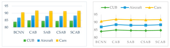
Figure 11.
The results of our proposed method, histogram (left) and polygonal chart (right) can intuitively show the accuracy difference of all theories on different datasets.
The accuracy of the theory presented in this paper is higher than that of BCNN, where CAB and SCAB are the most improved, which shows that the attention mechanism can improve the ability of the model to model local special features to some extent. CAB is optimal on all datasets while the accuracy of CSAB is relatively low, indicating that the single-channel attention mechanism can effectively improve the local modeling ability of the model by increasing the weight of the discriminative region, but spatial attention will weaken the ability of local modeling of the channel attention. In contrast, the accuracy of RSCA is better than SAB, indicating that channel attention will enhance the ability of local modeling of spatial attention.
4.2.4. Ablation Study
The proposed attention mechanism mainly consists of an attention mode and a superposition mode. To investigate the effectiveness of different modes, we conducted ablation experiments on CUB-200-2011.
As shown in Table 7, first, we observe that all configurations outperform the baseline BCNN with at least a 0.2% margin. It shows the effectiveness of our framework. Second, when using only one mode, both attention mode and a superposition mode (initial BCNN) performed worse than their combination. More specifically, adding attention mode achieved accuracies with improvement from 0.2 to 0.5, while initial BCNN brought zero performance gains, which showed that the attention mode and superposition mode are mutually correlated and can reinforce each other. It means both of the two modes are essential for attention mechanism.
Table 7.
Ablation study of different mode on CUB-200-2011.
5. Conclusions
In this paper, we present a novel attention bilinear pooling model, which fuses attention and bilinear pooling for better classification. The attention mechanism can divide into channel and spatial wise attention. We discuss their differences in detail. Extensive experiments demonstrated the effectiveness of our theory and then provide discussions on it. In the future, we will conduct extended research in two directions, i.e., how to effectively to focus on a local object to obtain part representation, and how to improve bilinear pooling.
Author Contributions
Formal analysis, W.W.; methodology, W.W.; software, F.W. and W.W.; writing—original draft, W.W.; writing—review and editing, J.Z.; project administration, W.W., J.Z. and F.W.; funding acquisition, J.Z.
Funding
This research was funded by the National Natural Science Foundation of China (NSFC) with grant number 6117019.
Conflicts of Interest
The authors declare no conflict of interest.
References
- Girshick, R.; Donahue, J.; Darrell, T.; Malik, J. Rich feature hierarchies for accurate object detection and semantic segmentation. In Proceedings of the IEEE Conference on Computer Vision and Pattern Recognition, Columbus, OH, USA, 24–27 June 2014; pp. 580–587. [Google Scholar]
- Girshick, R. Fast R-CNN. In Proceedings of the IEEE International Conference on Computer Vision, Santiago, Chile, 7–13 December 2015; pp. 1440–1448. [Google Scholar]
- Ren, S.; He, K.; Girshick, R.; Sun, J. Faster r-cnn: Towards real-time object detection with region proposal networks. In Proceedings of the Advances in Neural Information Processing Systems, Montreal, QC, Canada, 7–12 December 2015; pp. 91–99. [Google Scholar]
- Uijlings, J.R.R.; Van De Sande, K.E.A.; Gevers, T.; Smeulders, A.W.M. Selective Search for Object Recognition. Int. J. Comput. Vis. 2013, 104, 154–171. [Google Scholar] [CrossRef]
- Sermanet, P.; Eigen, D.; Zhang, X.; Mathieu, M.; Fergus, R.; LeCun, Y. Overfeat: Integrated recognition, localization and detection using convolutional networks. arXiv 2013, arXiv:1312.6229. [Google Scholar]
- Chang, Y.L.; Liu, J.N.; Han, C.C.; Chen, Y.N. Hyperspectral image classification using nearest feature line embedding approach. IEEE Trans. Geosci. Remote Sens. 2013, 52, 278–287. [Google Scholar] [CrossRef]
- Tang, K.; Paluri, M.; Fei-Fei, L.; Fergus, R.; Bourdev, L. Improving image classification with location context. In Proceedings of the IEEE International Conference on Computer Vision, Santiago, Chile, 7–13 December 2015; pp. 1008–1016. [Google Scholar]
- Ristin, M.; Gall, J.; Guillaumin, M.; Van Gool, L. From categories to subcategories: Large-scale image classification with partial class label refinement. In Proceedings of the IEEE Conference on Computer Vision and Pattern Recognition, Boston, MA, USA, 7–12 June 2015; pp. 231–239. [Google Scholar]
- Wah, C.; Branson, S.; Welinder, P.; Perona, P.; Belongie, S. The Caltech-UCSD Birds-200–2011 Dataset; California Institute of Technology: Pasadena, CA, USA, 2011. [Google Scholar]
- Zhang, N.; Donahue, J.; Girshick, R.; Darrell, T. Part-based R-CNNs for fine-grained category detection. In Proceedings of the European conference on computer vision, Zurich, Switzerland, 6–12 September 2014; Springer: Cham, Switzerland, 2014; pp. 834–849. [Google Scholar]
- Chéron, G.; Laptev, I.; Schmid, C. P-cnn: Pose-based cnn features for action recognition. In Proceedings of the IEEE International Conference on Computer Vision, Santiago, Chile, 7–13 December 2015; pp. 3218–3226. [Google Scholar]
- Wei, X.S.; Xie, C.W.; Wu, J. Mask-cnn: Localizing parts and selecting descriptors for fine-grained image recognition. arXiv 2016, arXiv:1605.06878. [Google Scholar]
- Lin, T.Y.; RoyChowdhury, A.; Maji, S. Bilinear cnn models for fine-grained visual recognition. In Proceedings of the IEEE International Conference on Computer Vision, Santiago, Chile, 7–13 December 2015; pp. 1449–1457. [Google Scholar]
- Gao, Y.; Beijbom, O.; Zhang, N.; Darrell, T. Compact bilinear pooling. In Proceedings of the IEEE Conference on Computer Vision and Pattern Recognition, Las Vegas, NV, USA, 27–30 June 2016; pp. 317–326. [Google Scholar]
- Cui, Y.; Zhou, F.; Wang, J.; Liu, X.; Lin, Y.; Belongie, S. Kernel pooling for convolutional neural networks. In Proceedings of the IEEE Conference on Computer Vision and Pattern Recognition, Honolulu, HI, USA, 21–26 July 2017; pp. 2921–2930. [Google Scholar]
- Kong, S.; Fowlkes, C. Low-rank bilinear pooling for fine-grained classification. In Proceedings of the IEEE Conference on Computer Vision and Pattern Recognition, Honolulu, HI, USA, 21–26 July 2017; pp. 365–374. [Google Scholar]
- Li, Y.; Wang, N.; Liu, J.; Hou, X. Factorized bilinear models for image recognition. In Proceedings of the IEEE International Conference on Computer Vision, Venice, Italy, 22–29 October 2017; pp. 2079–2087. [Google Scholar]
- Cai, S.; Zuo, W.; Zhang, L. Higher-order integration of hierarchical convolutional activations for fine-grained visual categorization. In Proceedings of the IEEE International Conference on Computer Vision, Venice, Italy, 22–29 October 2017; pp. 511–520. [Google Scholar]
- Krause, J.; Stark, M.; Jia, D.; Li, F.F. 3D Object Representations for Fine-Grained Categorization. In Proceedings of the IEEE International Conference on Computer Vision, Sydney, NSW, Australia, 2–8 December 2013; pp. 554–561. [Google Scholar]
- Maji, S.; Rahtu, E.; Kannala, J.; Blaschko, M.; Vedaldi, A. Fine-grained visual classification of aircraft. arXiv 2013, arXiv:1306.5151. [Google Scholar]
- Hu, J.; Shen, L.; Sun, G. Squeeze-and-excitation networks. In Proceedings of the IEEE Conference on Computer Vision and Pattern Recognition, Salt Lake City, UT, USA, 18–22 June 2018; pp. 7132–7141. [Google Scholar]
- Rida, I.; Al-Maadeed, N.; Al-Maadeed, S.; Bakshi, S. A comprehensive overview of feature representation for biometric recognition. Multimed. Tools Appl. 2018, 1–24. [Google Scholar] [CrossRef]
- Krizhevsky, A.; Sutskever, I.; Hinton, G.E. Imagenet classification with deep convolutional neural networks. In Proceedings of the Advances in Neural Information Processing Systems, Lake Tahoe, NV, USA, 3–6 December 2012; pp. 1097–1105. [Google Scholar]
- Simonyan, K.; Zisserman, A. Very deep convolutional networks for large-scale image recognition. arXiv 2014, arXiv:1409.1556. [Google Scholar]
- Kar, P.; Karnick, H. Random feature maps for dot product kernels. In Proceedings of the Artificial Intelligence and Statistics, La Palma, Canary Islands, Spain, 21–23 April 2012; pp. 583–591. [Google Scholar]
- Pham, N.; Pagh, R. Fast and scalable polynomial kernels via explicit feature maps. In Proceedings of the 19th ACM SIGKDD International Conference on Knowledge Discovery and Data Mining, Chicago, IL, USA, 11–14 August 2013; pp. 239–247. [Google Scholar]
- Fu, J.; Zheng, H.; Mei, T. Look closer to see better: Recurrent attention convolutional neural network for fine-grained image recognition. In Proceedings of the IEEE Conference on Computer Vision and Pattern Recognition, Honolulu, HI, USA, 21–26 July 2017; pp. 4438–4446. [Google Scholar]
- Zheng, H.; Fu, J.; Mei, T.; Luo, J. Learning multi-attention convolutional neural network for fine-grained image recognition. In Proceedings of the IEEE International Conference on Computer Vision, Venice, Italy, 22–29 October 2017; pp. 5209–5217. [Google Scholar]
- Mnih, V.; Heess, N.; Graves, A. Recurrent models of visual attention. In Proceedings of the Advances in Neural Information Processing Systems, Montreal, QC, USA, 8–13 December 2014; pp. 2204–2212. [Google Scholar]
- Gregor, K.; Danihelka, I.; Graves, A.; Rezende, D.J.; Wierstra, D. Draw: A recurrent neural network for image generation. arXiv 2015, arXiv:1502.04623. [Google Scholar]
- Ba, J.; Mnih, V.; Kavukcuoglu, K. Multiple object recognition with visual attention. arXiv 2014, arXiv:1412.7755. [Google Scholar]
- Zhang, Q.; Yang, Y.; Ma, H.; Wu, Y.N. Interpreting cnns via decision trees. In Proceedings of the IEEE Conference on Computer Vision and Pattern Recognition, Long Beach, CA, USA, 15–20 June 2019; pp. 6261–6270. [Google Scholar]
- Woo, S.; Park, J.; Lee, J.Y.; So Kweon, I. Cbam: Convolutional block attention module. In Proceedings of the European Conference on Computer Vision (ECCV), Munich, Germany, 8–14 September 2018; pp. 3–19. [Google Scholar]
- Wei, X.S.; Luo, J.H.; Wu, J.; Zhou, Z.H. Selective convolutional descriptor aggregation for fine-grained image retrieval. IEEE Trans. Image Process. 2017, 26, 2868–2881. [Google Scholar] [CrossRef] [PubMed]
- Lin, M.; Chen, Q.; Yan, S. Network in network. arXiv 2013, arXiv:1312.4400. [Google Scholar]
- Szegedy, C.; Ioffe, S.; Vanhoucke, V.; Alemi, A.A. Inception-v4, inception-resnet and the impact of residual connections on learning. In Proceedings of the Thirty-First AAAI Conference on Artificial Intelligence, San Francisco, CA, USA, 4–9 February 2017. [Google Scholar]
- Szegedy, C.; Liu, W.; Jia, Y.; Sermanet, P.; Reed, S.; Anguelov, D.; Rabinovich, A. Going deeper with convolutions. In Proceedings of the IEEE Conference on Computer Vision and Pattern Recognition, Boston, MA, USA, 7–12 June 2015; pp. 1–9. [Google Scholar]
- Morgado, P.; Vasconcelos, N. NetTailor: Tuning the Architecture, Not Just the Weights. In Proceedings of the IEEE Conference on Computer Vision and Pattern Recognition, Long Beach, CA, USA, 15–20 June 2019; pp. 3044–3054. [Google Scholar]
- Russakovsky, O.; Deng, J.; Su, H.; Krause, J.; Satheesh, S.; Ma, S.; Berg, A.C. Imagenet large scale visual recognition challenge. Int. J. Comput. Vis. 2015, 115, 211–252. [Google Scholar] [CrossRef]
© 2019 by the authors. Licensee MDPI, Basel, Switzerland. This article is an open access article distributed under the terms and conditions of the Creative Commons Attribution (CC BY) license (http://creativecommons.org/licenses/by/4.0/).