Article

From Symmetry to Asymmetry on the Disc Manifold: Modeling of Marion Island Data

1
Department of Statistics, University of Pretoria, Pretoria 0002, South Africa
2
Department of Statistics, Faculty of Mathematical Sciences, Shahrood University of Technology, Shahrood 3619995161, Iran
3
Faculty of Natural Sciences, Akademia, and School of Health Systems and Public Health, University of Pretoria, Pretoria 0002, South Africa
*
Author to whom correspondence should be addressed.
Symmetry 2019, 11(8), 1030; https://doi.org/10.3390/sym11081030
Submission received: 28 June 2019 / Revised: 5 August 2019 / Accepted: 6 August 2019 / Published: 9 August 2019
(This article belongs to the Special Issue Recent Advances on Symmetry in Mathematical Statistics)

Abstract

:
The joint modeling of angular and linear observations is crucial as data of this nature are prevalent in multiple disciplines, for example the joint modeling of wind direction and another climatological variable such as wind speed or air temperature, the direction an animal moves and the distance moved, or wave direction and wave height. Hence, there is a need for developing flexible distributions on the hyper-disc, which has support of the interior of the hyper-sphere, as it allows for modeling the combination of angular and linear observations. This paper addresses this need by developing flexible distributions for the disc that have the ability to capture any inherent bimodality present in the data. A new class of bivariate distributions is proposed which has support on the unit disc in two dimensions that includes, as a special case, the existing Möbius distribution on the disc. This class is obtained by expressing the density function in a general form using a measurable function termed as generator. Special cases of this generator are considered to demonstrate the flexibility. By applying a conformal mapping to the generator function a new Möbius distribution class emanates. This class of bivariate distributions on the disc is the first to account for bimodality and skewness present in the data. The flexible behavior of the proposed models in terms of bimodality and skewness is graphically demonstrated. Preliminary evidential analysis of the wind data observed at Marion Island reveals the absence of unimodality in the data. The fit of the proposed models, which account for bimodality, to the Marion Island wind data were evaluated analytically and visually.

Graphical Abstract

1. Introduction

The analytical description of wind climate is usually confined to the description of wind speed; however, the joint description of the directional and linear wind characteristics is also essential. This joint modeling of wind speed and direction is important for climatology and a variety of ocean engineering and ecological applications. Further emphasis on the necessity of bivariate modeling of wind speed and wind direction was raised by  [1]. One approach to capture both the linear and directional variables is by means of a disc. There are very few distributions available with support on the unit disc. To the best of the author’s knowledge, the only literature that investigates distributions on the hyper-disc are those by Jones [2,3] and Uesu, et al. [4]. In [2], the bivariate beta distribution was proposed for the disc which is a symmetric distribution. In [3], the Möbius distribution on the disc was proposed, which allowed for skewness. The multivariate extension of the Möbius distribution on the disc to the hyper-disc was then proposed by Uesu, et al. [4]. A shortcoming in the existing distributions on a disc is the ability to account for bimodality present in the data. There exists flexible distributions for cylindrical models as proposed in [5,6,7], but not the disc. The need for jointly modeling a linear and angular variable on a disc manifold stems from the cyclic nature of the angular variable which cannot be modeled the same as a linear variable. Many distributions have been proposed for modeling angular variables on a circle and other manifolds. For a full summary of these models, refer to the works of Mardia, et al. [8], Ley, et al. [9] and Pewsey, et al. [10].
In this paper, we propose a general framework for distributions which has support on the unit disc and includes the above-mentioned Möbius distribution on the disc [3] as a special case. This proposed class of the distributions accounts for both bimodality and skewness. We define this distribution by using a generator function and applying a conformal mapping, Möbius transformation, to obtain a new Möbius distribution class. This new class allows for bimodality when the generator function exhibits bimodal behavior with asymmetry introduced by the Möbius transformation.
An advantage of the proposed model is that it extends the shape characteristics of the model on the unit disc proposed by Jones [3] to account for more flexibility. This approach to modeling wind data differs from those in [1,11,12,13,14,15], by means of the correlation structure and method for obtaining the joint distribution. The aforementioned models have been built by means of: (i) the Johnson–Wehrly (JW) [7] method; and (ii) a copula approach where the univariate models of best fit are chosen to obtain a joint bivariate distribution for the wind speed and wind direction. The proposed model in this paper has an embedded correlation structure present to jointly account for the wind speed and wind direction. It was pointed out in [16] that the joint modeling of wind speed and wind direction is more significant than a univariate analysis of the wind speed. The univariate distribution of the wind speed or wind direction is not considered since Soukissian, et al. [1] pointed out that the best univariate distribution for wind speed does not provide the best bivariate fit for the wind speed and wind direction. There has been much attention of wind power assessment worldwide, however, there has been no analysis of the wind speed and wind direction analysis at Marion Island. The proposed models was used to analyse the wind data for Marion Island. These models were compared to the only known model on the disc, which is a special case of the proposed class. The main contributions of this paper can be summarized as follows:
  • A new class of distributions on the disc for the joint modeling of a linear and angular variable is introduced. This class includes as a special case the Möbius distribution on the disc. The class can assume a parametric or semi-parametric model based on the choice of the practitioner.
  • In the semi-parametric model, a general class is introduced. For this model, we propose a computational algorithm which simplifies to a univariate kernel density function in order to obtain the parameter estimates.
  • The proposed class of distributions includes an embedded correlation structure present in the model to account for any relation between the linear and angular variables. This is addresses a shortcoming in the joint modeling of linear and angular variables. The embedded correlation structure reduces any assumption of the univariate models for the linear and angular variables.
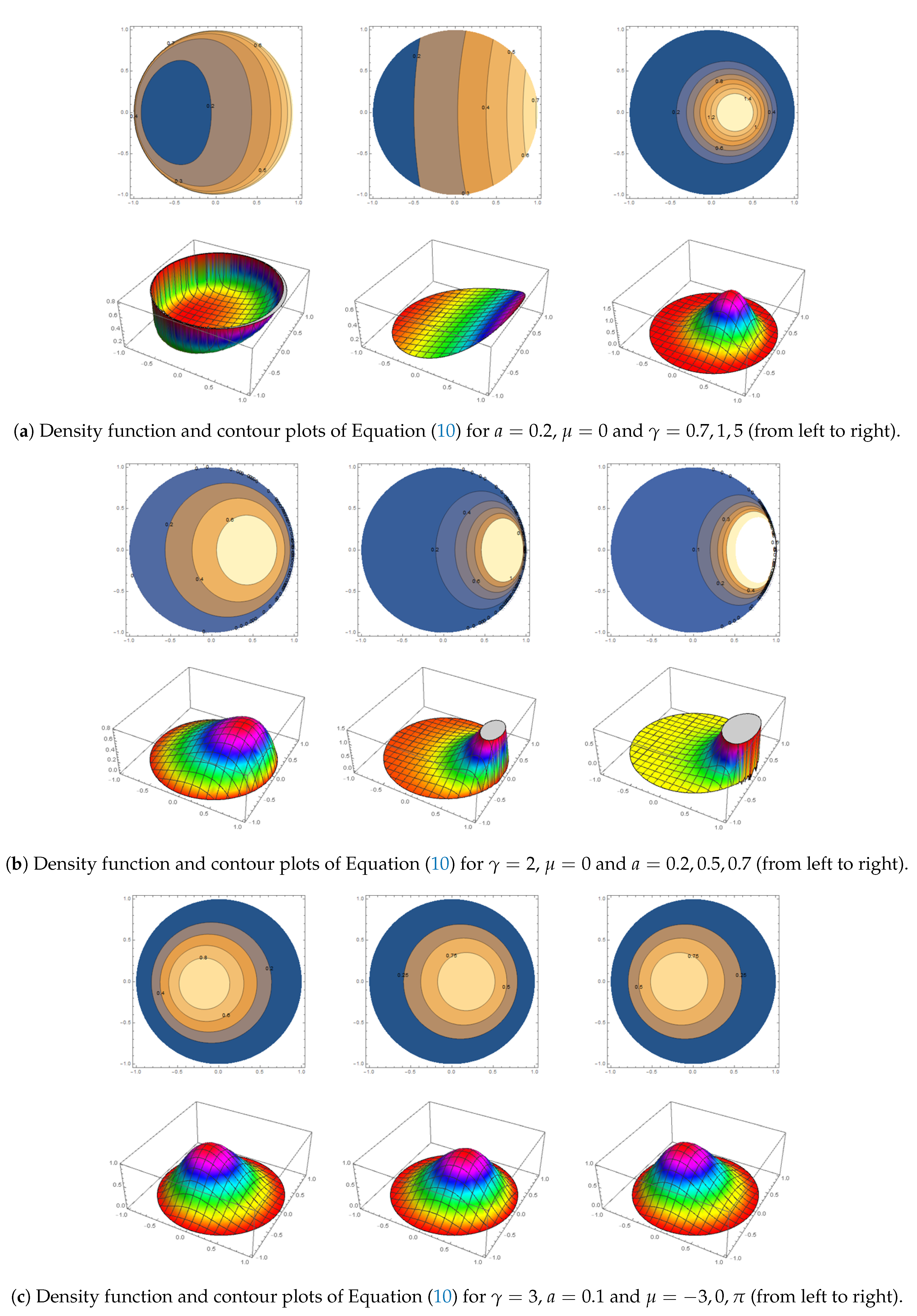
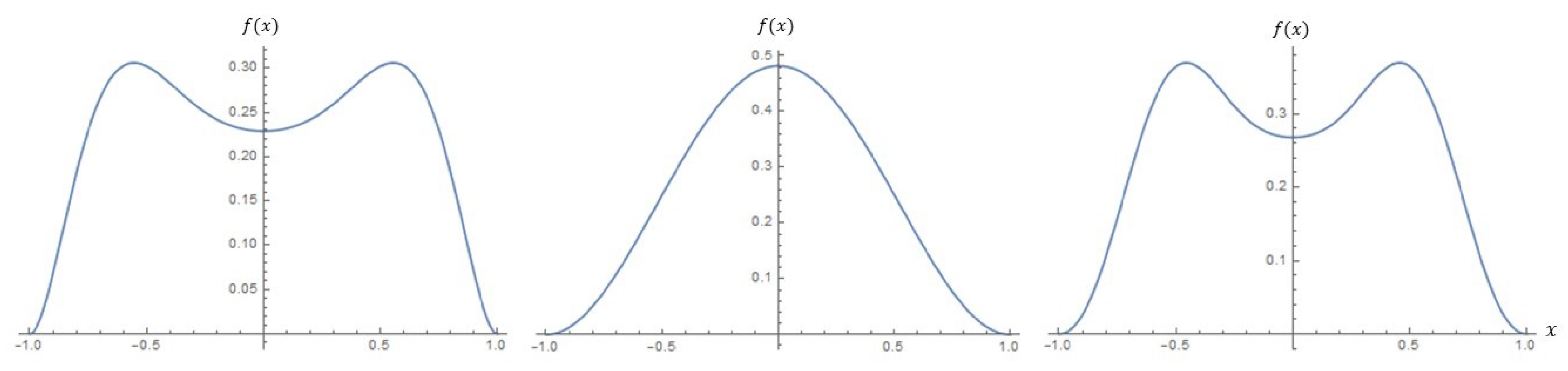
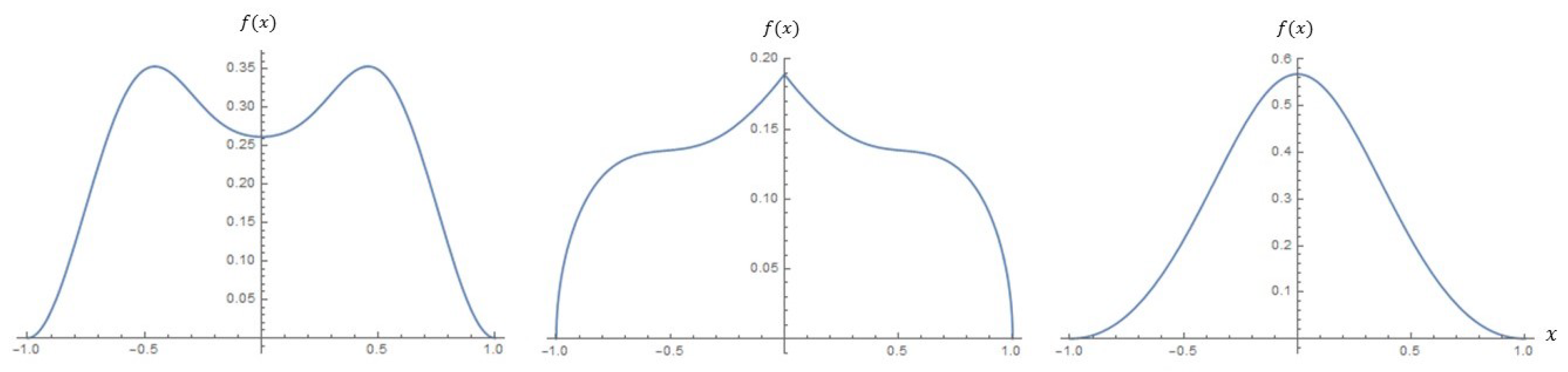
  • The need for flexible models on a disc is addressed by introducing a class of distributions that can account for bimodality and skewness present in the data. An advantage of the proposed model is that it extends the shape characteristics of the model on the unit disc proposed by Jones [3] to account for more flexibility.
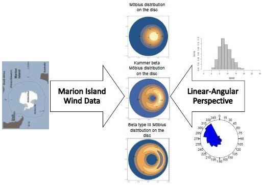
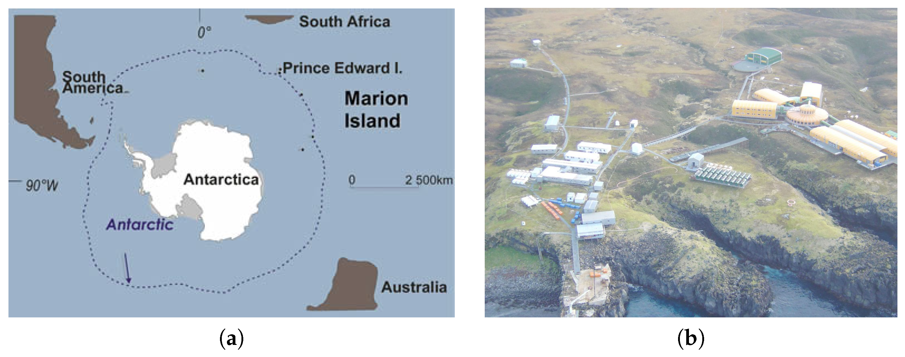
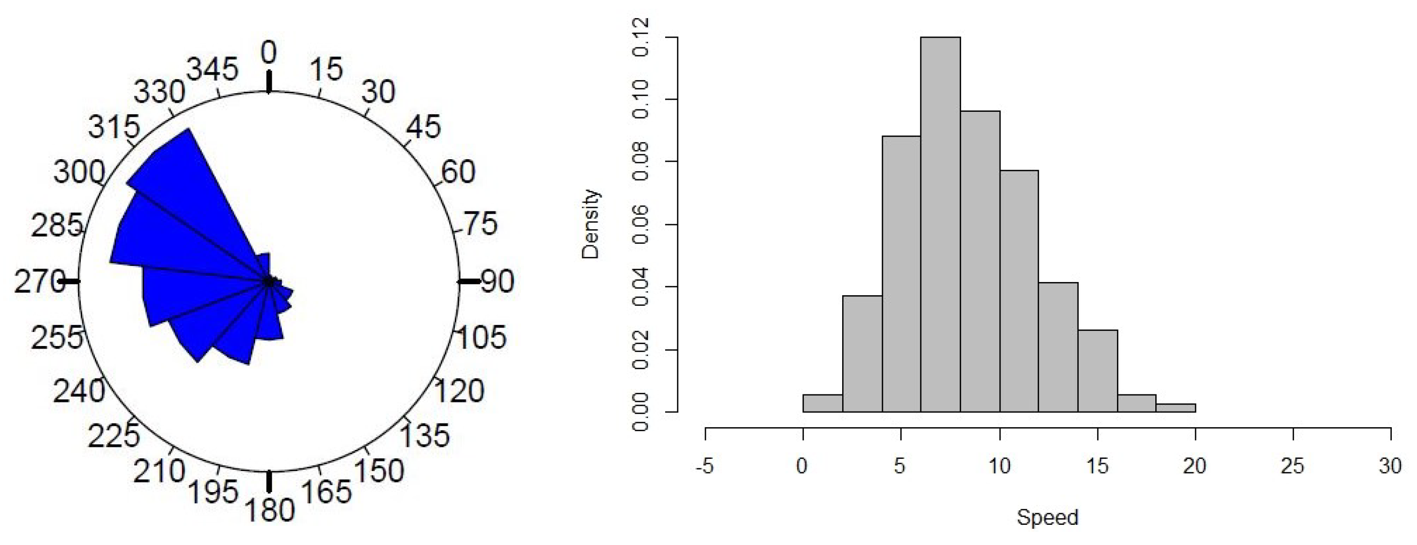
  • The modeling of the wind speed and wind direction data at Marion Island was jointly analyzed for the first time in this study.
This new class of distributions is defined in Section 3 and special cases of the generator function are highlighted in Section 4. In Section 5, an illustrative example of fitting the different models emanating from the class, to Marion Island wind data is presented. The numerical results along with the evaluation of the bivariate fits are also presented. Subsequently, a background discussion of the Marion Island weather data ia provided in Section 2. Section 6 concludes with a summary and some final remarks.

2. Background

The Prince Edward Island group (PEI) consist of two small volcanic islands: (1) Marion Island; and (2) Prince Edward Island. These islands are located in the sub-Antarctic Indian Ocean at latitude 46 49 –46 59 South and longitude 37 35 –37 55 East (see Figure 1a). Both island territories belong to South Africa, which is situated 1900 km to the northwest of the island group [17]. The recently declared PEIs Marine Protected Area (MPA) is one of the largest of its kind in the world and serves as a research area for South Africa as well as the world.
With an area of about 290 km 2 , a circumference of 72 km and the highest peak at 1300 m, Marion Island is the larger of the Prince Edward Islands. With its geographic isolation, Marion Island’s climate is highly oceanic in nature, coupled with the influence of passing frontal weather systems. This creates conditions of high temperature variability and where gale force winds can blow during most weeks of the year. In 1948, South Africa established a fully operational weather station on Marion Island (see Figure 1b) with continuous weather data records available since the early 1950s [18]. Due to its duration and the scarcity of weather data from the sub-Antarctic region, these weather records provide valuable and unique opportunities for research.
Data from the Marion Island describe climate variability collected by a weather station that is located near the coast on the eastern side of the island [19]. Wind differences between the eastern (predominantly leeward winds) and western (windward) parts of the island, both within the larger scale prevalence of westerly winds, have long been speculated about [19,20,21]. It has been suggested that winds at the western side of the island, where no consistent data collection exists, are stronger and less variable, in comparison to winds at the eastern weather station. Despite these orographically induced differences, wind recordings of the weather should capture the larger scale variability of climate at Marion Island.
The data used in this study were obtained from Marion Island and were recorded daily at 08:00, 14:00 and 20:00 SAST (relates to the main synoptic hours). The daily averages were obtained and the wind speed and wind direction investigated for nine different years. These nine years were considered in two-year intervals from 2001 to 2017. Figure 2 provides visual displays of the data to the reader with some background to the behavior of the data.
A scatter plot of the wind direction and wind speed is given in Figure 3.
In Table 1, the values of the main circular statistics [8] of the wind direction for the nine years are given. Specifically, the mean resultant length ( r ¯ ), mean direction ( θ ¯ ), circular variance ( V Θ ), circular standard deviation ( ν Θ ), circular dispersion ( δ ^ ), circular skewness ( s ^ ) and circular kurtosis ( k ^ ) are shown.

3. Construction Methodology

In this section, we define the general Möbius class and consider an algorithm to estimate the generator function and the parameters using a semi-parametric approach.

3.1. Möbius Transformation

The Möbius transformation is defined on the extended complex plane denoted by C ˜ [22]. Hence, we rewrite the cartesian coordinates in polar coordinates. Considering the polar coordinate form of the unit disc, we write z = x , y and w = u , v as complex numbers with w = r e i θ , 0 r 1 , π < θ π . The Möbius transformation is defined by [23] as
z = M c w = w c 1 c ¯ w with inverse w = M c z = z + c 1 + c ¯ z
where c = a e i μ , 0 a < 1 and c ¯ denotes the complex conjugate. The only conformal mapping from the unit disc to itself is the Möbius transformation [23]. Using this Möbius transformation, we can develop probability distributions [3,24,25].

3.2. Cartesian Coordinate Configuration of the General Class

Consider the general bivariate density function,
f x , y = C g x 2 + y 2 ,
where 0 x 2 + y 2 1 and g ( · ) is a continuous function termed as the “generator”. The normalizing constant C can be obtained from the polar form of Equation (1) as
C 1 = 0 2 π 0 1 s g s 2 d s d ϕ = 2 π 0 1 1 2 g u d u = π 0 1 g u d u ,
when the g ( · ) function is infinitely differentiable at the point zero. Numerical computation of the integral in Equation (2) is given by
0 1 g u d u = E U ( 0 , 1 ) [ g ( X ) ] .
where E [ · ] denotes the expected value of a random variable. Writing the Taylor’s series expansion of g u in Equation (2) around zero gives
C 1 = π k = 0 g ( k ) ( 0 ) k ! 0 1 u k d u = π k = 0 g ( k ) ( 0 ) ( k + 1 ) ! ,
which allows the computation of the normalizing constant by derivatives of g ( · ) around zero.

3.3. A New Möbius Distribution Class on the Disc

By applying the Möbius transformation in Section 3.1, we obtain the class of general Möbius distributions on the disc as,
f r , θ = C 1 a 2 2 r π 1 2 a r cos θ μ + a 2 r 2 2 g a 2 2 a r cos θ μ + r 2 1 2 a r cos θ μ + a 2 r 2 .
where 0 a < 1 , π < μ π and 0 r 1 , π < θ π . We denote this class as r , θ G M a , μ , g .
Trivial calculations reveal for a strictly increasing generator function, L < f ( r , θ ) < U , where
L = C ( 1 a 2 ) 2 r π ( 1 + a r ) 4 g ( a r ) 2 ( 1 + a r ) 2 , U = C ( 1 + a 2 ) 2 r π ( 1 a r ) 4 g ( a + r ) 2 ( 1 a r ) 2 .
These bounds are achieved when θ = μ ( + π ) . For the limiting case a 0 , the joint distribution tends to C r g r 2 / π . We can rewrite the density function in Equation (4) in the Cartesian space by performing the transformation: u = r cos θ and v = r sin θ . Then, the resulting density function is
f u , v = C 1 a 2 2 π 1 2 a u cos μ 2 a v sin μ + a 2 u 2 + v 2 2 g a 2 2 a u cos μ 2 a v sin μ + u 2 + v 2 1 2 a u cos μ 2 a v sin μ + a 2 u 2 + v 2 ,
where 0 u 2 + v 2 1 , 0 a < 1 and π < μ π .

3.4. Maximum Likelihood Estimation

In this section, we derive the maximum likelihood (ML) estimates of the parameters. Let  S = r i , θ i i = 1 n be a random sample from G M a , μ , g , where all parameters are unknown. The likelihood function has the form
L a , μ , g = C 1 a 2 2 π n i = 1 n r i g a 2 2 a r i cos θ i μ + r i 2 1 2 a r i cos θ i μ + a 2 r i 2 1 2 a r i cos θ i μ + a 2 r i 2 2 .
Computational stages for estimating g ( · ) and the parameters are given by Algorithm 1.
Algorithm 1 ML estimation algorithm
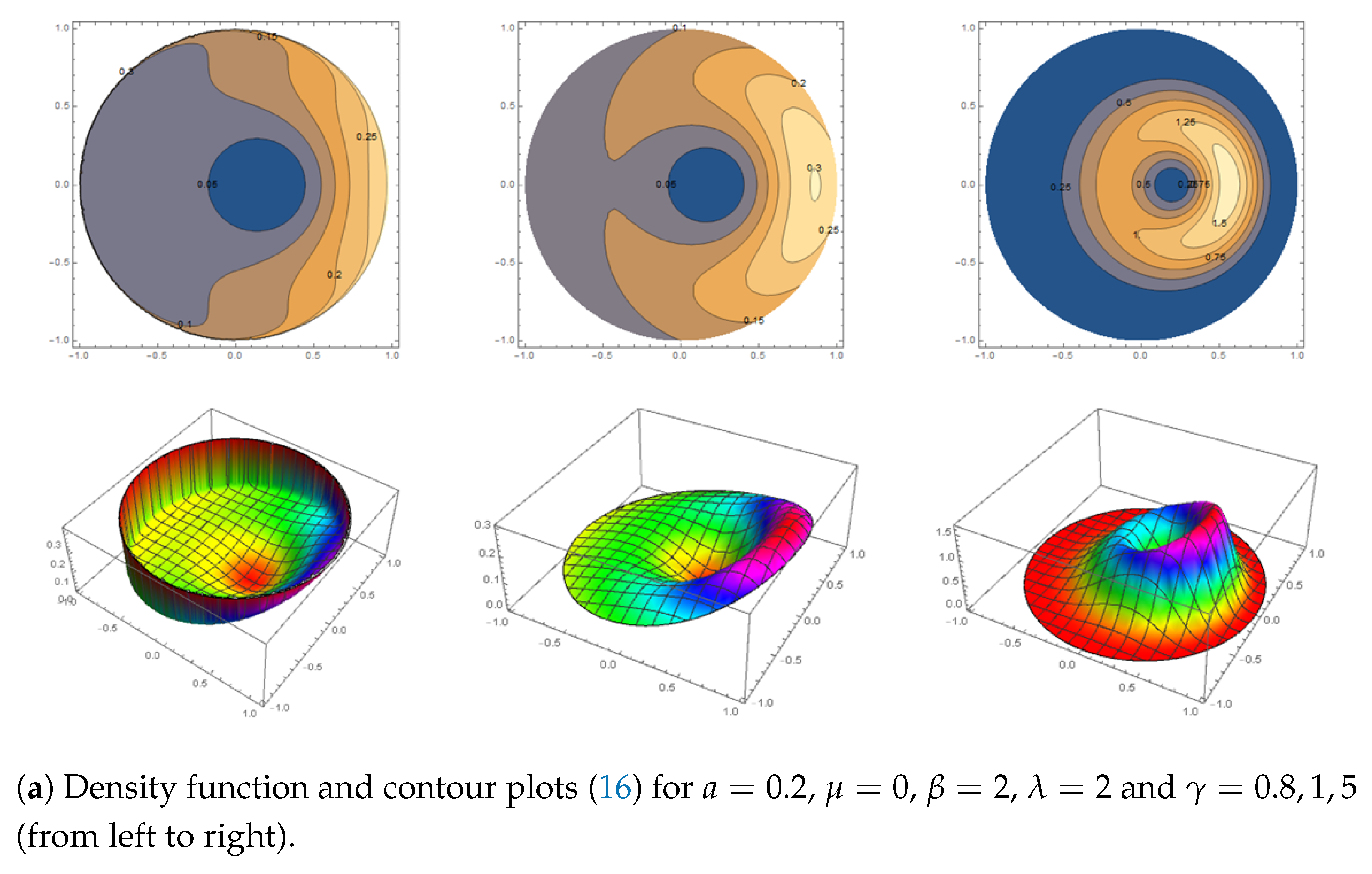
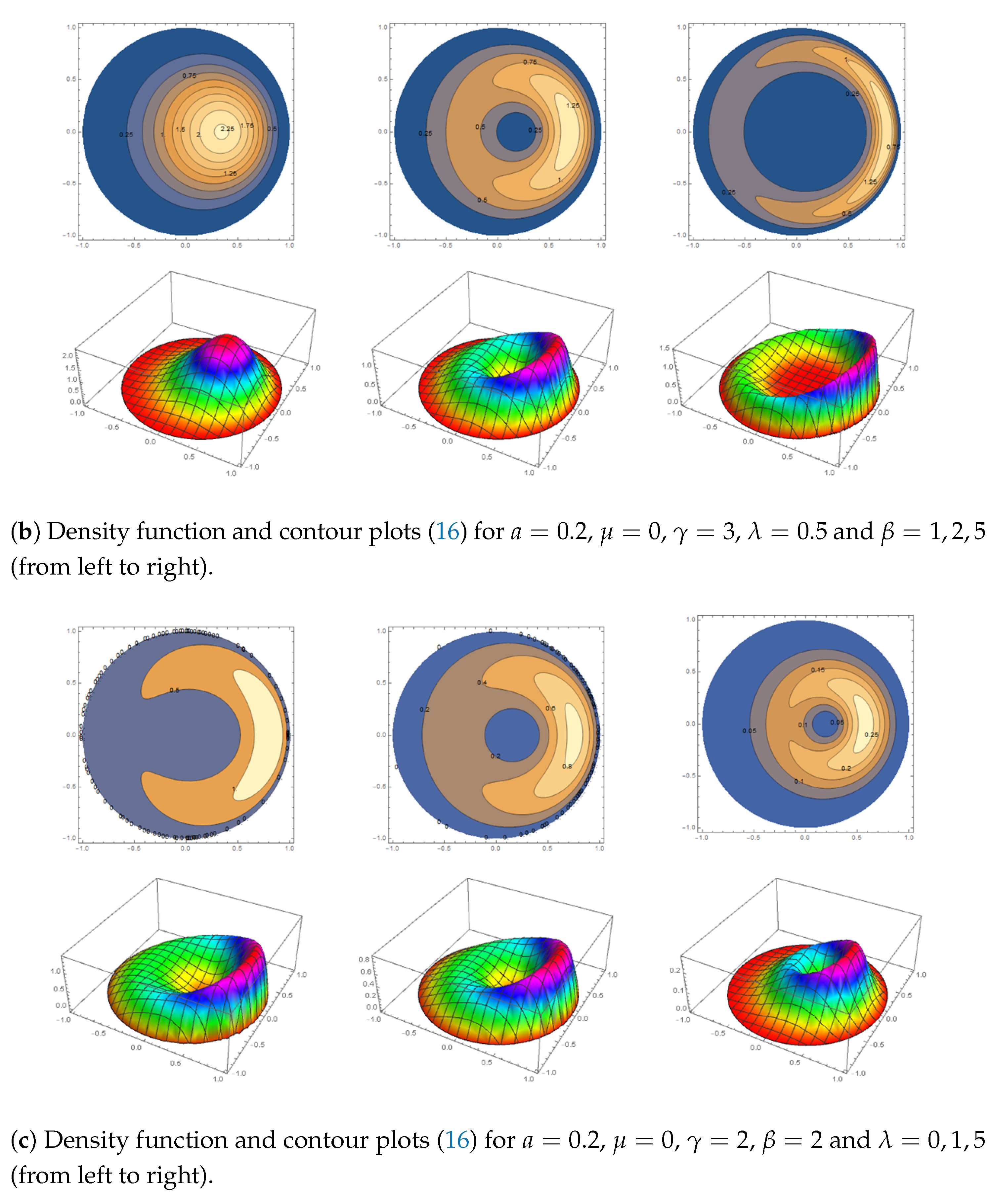
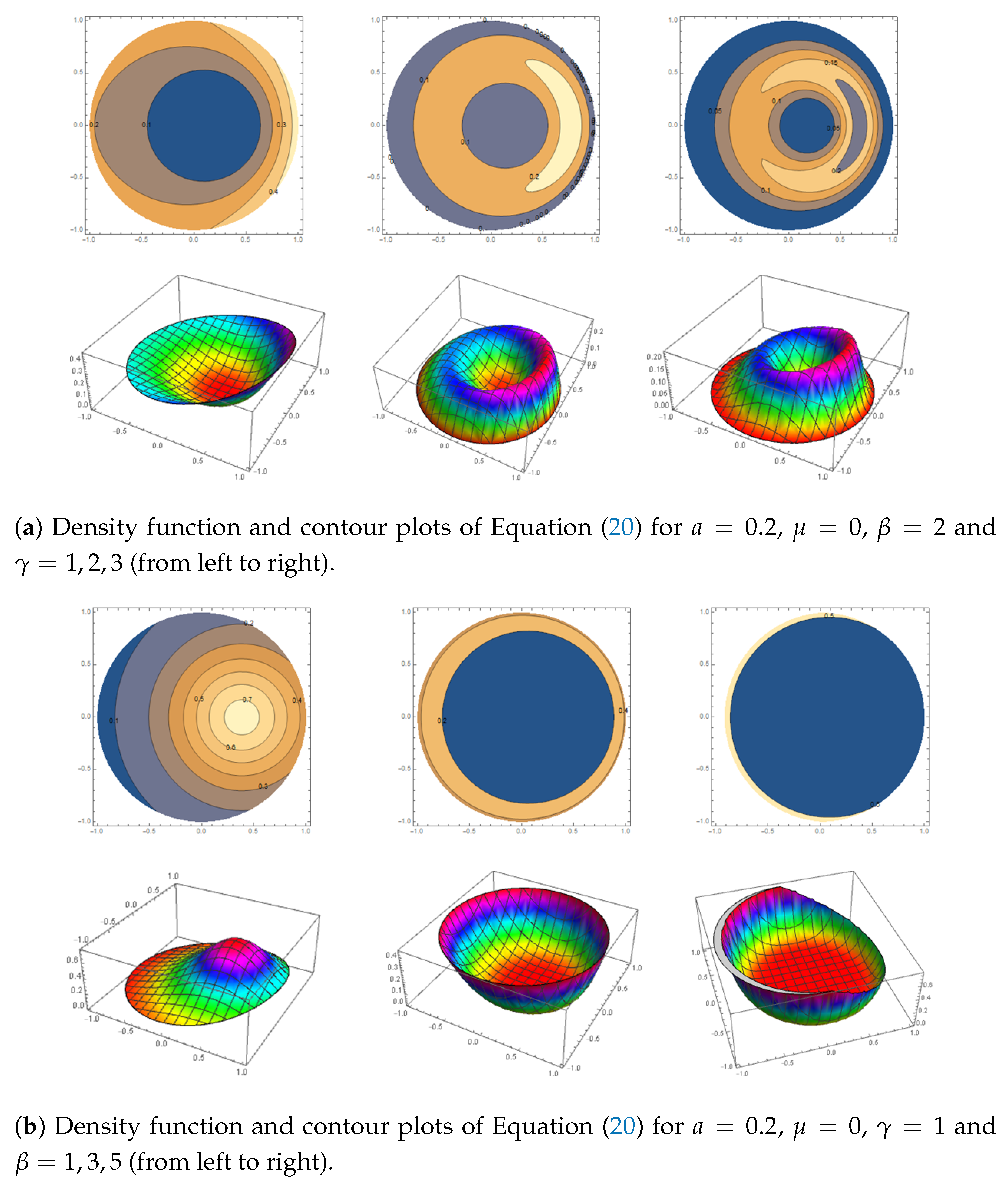
 Step 1. 
Set the initial values for the unknown parameters a ^ = 0 and μ ^ = π . These values are chosen as the lower bound as the algorithm performs an ascending sequential search through all possible parameter values.     
 Step 2. 
Given the observations ( r 1 , θ 1 ) , ( r 2 , θ 2 ) , , ( r n , θ n ) , we estimate g ( · ) via
g ^ x = 1 n h k = 0 n K x x i h ,
where x i = ( a 2 2 a r i cos θ i μ + r i 2 ) / ( 1 2 a r i cos θ i μ + a 2 r i 2 ) , h is the bandwidth and K ( · ) is the kernel function.     
 Step 3. 
Compute the likelihood function, Equation (7), using the estimated g ^ ( · ) , a ^ and μ ^ .     
 Step 4. 
Repeat Steps 2 and 3, using an optimization technique to achieve convergence for the parameters a and μ . The final estimated values are those that maximize the likelihood function.  
In Algorithm 1, the bandwidth h can be obtained using existing methods since the values in the argument of g ( · ) function belong to the Cartesian space. Hence, in our numerical studies, we applied the commonly used cross validation method to optimize h. Furthermore, we considered the standard Gaussian model for the kernel function, K ( · ) . In Algorithm 1, the computation time can be improved by considering a grid approach in Step 4 over the domain of the two parameters.
Remark 1.
The mathematical expressions for the modality of the model are intractable.

4. Special Cases

In this section, we consider three special cases of the generator function, g ( · ) . The first generator function, Pearson Type II distribution [26], results in the well known Möbius distribution on the disc proposed by Jones [3]. The second generator function, Kummer beta distribution [27], results in the Kummer beta Möbius distribution and the third generator function, beta type III distribution [28], results in the beta type III Möbius distribution. The Pearson Type II distribution was used for comparsion purposes and to show that the proposed new class of distributions include the well known distribution on the disc [3]. The other special cases are considered due to their flexibility and the capacity of the distribution to handle bimodality [27].

4.1. Möbius Distribution on the Disc

By defining the generator function as
g ( w ) = 1 w γ 1 ,
we obtain the bivariate spherically symmetric beta (Pearson Type II) distribution [26], with density function,
f γ x , y = γ π 1 x 2 y 2 γ 1 ,
where C = γ π > 0 , 0 x 2 + y 2 1 .
The density function and marginal distribution graphs in Figure 4 and Figure 5 illustrate the symmetrical and unimodal behavior of the generator function in Equation (8).
After applying the Möbius transformation, this choice of generator function in Equation (8) simplifies to the well known Möbius distribution on the disc defined by Jones [3].
The polar form density is given as
f r , θ = γ 1 a 2 γ + 1 r 1 r 2 γ 1 π 1 2 a r cos θ μ + a 2 r 2 γ + 1 ,
where 0 a < 1 , π < μ π , 0 r 1 and π < θ π . The density function in terms of Cartesian coordinates is
f u , v = γ 1 a 2 γ + 1 u 2 + v 2 1 2 1 u 2 v 2 γ 1 π 1 2 a u cos μ 2 a v sin μ + a 2 u 2 + v 2 γ + 1 ,
where 0 a < 1 , π < μ π and 0 u 2 + v 2 1 .
The parameters can be interpreted as γ controls the concentration, a controls the skewness (or the asymmetry for the length from the center of the disc) and μ controls the orientation of the distribution (see Figure 6).

Maximum Likelihood Estimation

The log-likelihood of the polar form density function, Equation (9), is obtained for maximum likelihood estimation as:
log L f r , θ = n log γ + n γ + 1 log 1 a 2 + i = 1 2 log r i + i = 1 2 γ 1 log 1 r i 2 n log π i = 1 2 γ + 1 log 1 2 a r i cos θ i μ + a 2 r i

4.2. Kummer Beta Möbius Distribution on the Disc

Consider the following generator function
g ( w ) = w β 1 1 w γ 1 exp λ w ,
where γ , β , λ > 0 . By substituting the generator function in Equation (1), the resulting distribution is a bivariate Kummer beta distribution [27] with density function
f γ , λ , β x , y = C x 2 + y 2 β 1 1 x 2 y 2 γ 1 exp λ x 2 + y 2 ,
where γ , β , λ > 0 , 0 x 2 + y 2 1 and
C = Γ β + γ π Γ β Γ γ 1 F 1 β , β + γ , λ
is the normalizing constant where 1 F 1 ( · ) is the confluent hypergeometric function of the first kind [29].
The density function and marginal distribution graphs in Figure 7 and Figure 8 illustrate the symmetrical and bimodal behavior of the generator function.
After applying the inverse Möbius transformation in Section 3.1, the Kummer beta Möbius distribution is obtained from Equation (4) with the density function in terms of the polar coordinates as
f r , θ = C r 1 a 2 γ + 1 1 r 2 γ 1 a 2 2 a r cos θ μ + r 2 β 1 × exp λ a 2 2 a r cos θ μ + r 2 1 2 a r cos θ μ + a 2 r 2 × 1 2 a r cos θ μ + a 2 r 2 γ β ,
where 0 a < 1 , π < μ π , 0 r 1 , π < θ π and C given by Equation (13).
We can obtain the density function in terms of Cartesian coordinates u , v by using Equation (6), thus the density function is
f u , v = C 1 a 2 γ + 1 1 u 2 v 2 γ 1 a 2 2 a u cos μ 2 a v sin μ + u 2 + v 2 β 1 × exp λ a 2 2 a u cos μ 2 a v sin μ + u 2 + v 2 1 2 a u cos μ 2 a v sin μ + a 2 u 2 + v 2 × 1 2 a u cos μ 2 a v sin μ + a 2 u 2 + v 2 γ β ,
where 0 u 2 + v 2 1 , 0 a < 1 , π < μ π and C is given by Equation (13).
The parameters can be interpreted as γ controls the concentration, while β contributes to the concentration by adding bimodality. As the value of β increases, the model introduces another mode in the form of an antimode, as seen in the plots of the generator function in Figure 7. The parameter λ controls the steepness of the concentration, a controls the skewness (or the asymmetry for the length from the center of the disc) and μ controls the orientation of the distribution (see Figure 9).

Maximum Likelihood Estimation

The log-likelihood of the polar form density function, Equation (15), is obtained for maximum likelihood estimation as:
log L f r , θ = n log Γ γ + β n log Γ β n log Γ γ n log 1 F 1 β , β + γ , λ n log π + n γ + 1 log 1 a 2 + γ 1 i = 1 n log 1 r i 2 + i = 1 n log r i + β 1 i = 1 n log a 2 2 a r i cos θ i μ + r i 2 γ + β i = 1 n log 1 2 a r i cos θ i μ + a 2 r i 2 λ i = 1 n a 2 2 a r i cos θ i μ + r i 2 1 2 a r i cos θ i μ + a 2 r i 2 .

4.3. Beta Type III Möbius Distribution on the Disc

Consider the following generator function
g ( w ) = w β 1 1 w γ 1 1 + w ( γ + β ) ,
where γ , β > 0 . By substituting the generator in Equation (1), the resulting distribution is a bivariate Beta type III distribution [28] with density function
f γ , β x , y = C x 2 + y 2 β 1 1 x 2 y 2 γ 1 1 + x 2 + y 2 γ + β ,
where γ , β > 0 , 0 x 2 + y 2 1 and
C = 2 β Γ β + γ π Γ β Γ γ
is the normalizing constant.
The density function and marginal distribution graphs in Figure 10 and Figure 11 illustrate the symmetrical and bimodal behavior of the generator function.
After applying the inverse Möbius transformation in Section 3.1, the Beta type III Möbius distribution is obtained from Equation (4) with the density function in terms of the polar coordinates as
f r , θ = C r 1 a 2 γ + 1 1 r 2 γ 1 a 2 2 a r cos θ μ + r 2 β 1 × 1 + r 2 1 + a 2 4 a r cos θ μ γ β ,
where 0 a < 1 , π < μ π , 0 r 1 , π < θ π and C as given in Equation (18).
We can obtain the density function in terms of Cartesian coordinates u , v by using Equation (6), thus the density function is
f u , v = C 1 a 2 γ + 1 1 u 2 v 2 γ 1 a 2 2 a u cos μ 2 a v sin μ + u 2 + v 2 β 1 × 1 + u 2 + v 2 1 + a 2 4 a u cos μ 4 a v sin μ γ β
where 0 u 2 + v 2 1 , 0 a < 1 , π < μ π and C is given in Equation (18).
The parameters can be interpreted as γ controls the steepness of the concentration, while β contributes to the concentration by adding bimodality. As the value of β increases ( β > 1 ), the model introduces another mode in the form of an antimode, as seen in the generator function plots in Figure 10. The parameters a controls the skewness (or the asymmetry for the length from the center of the disc) and μ controls the orientation of the distribution (see Figure 12).

Maximum Likelihood Estimation

The log-likelihood of the polar form density function, Equation (19), is obtained for maximum likelihood estimation as:
log L f r , θ = n β log 2 + n log Γ λ + β n log Γ β n log Γ λ n log π + i = 1 n log r i + n γ + 1 log 1 a 2 + γ 1 i = 1 n log 1 r i 2 + β 1 i = 1 n log a 2 2 a r i cos θ i μ + r i 2 γ + β i = 1 n log 1 + a 2 1 + r i 2 4 a r i cos θ i μ .
Remark 2.
The marginal distributions for our proposed models are intractable. Obtaining the marginal distribution via numerical integration is computationally expensive.

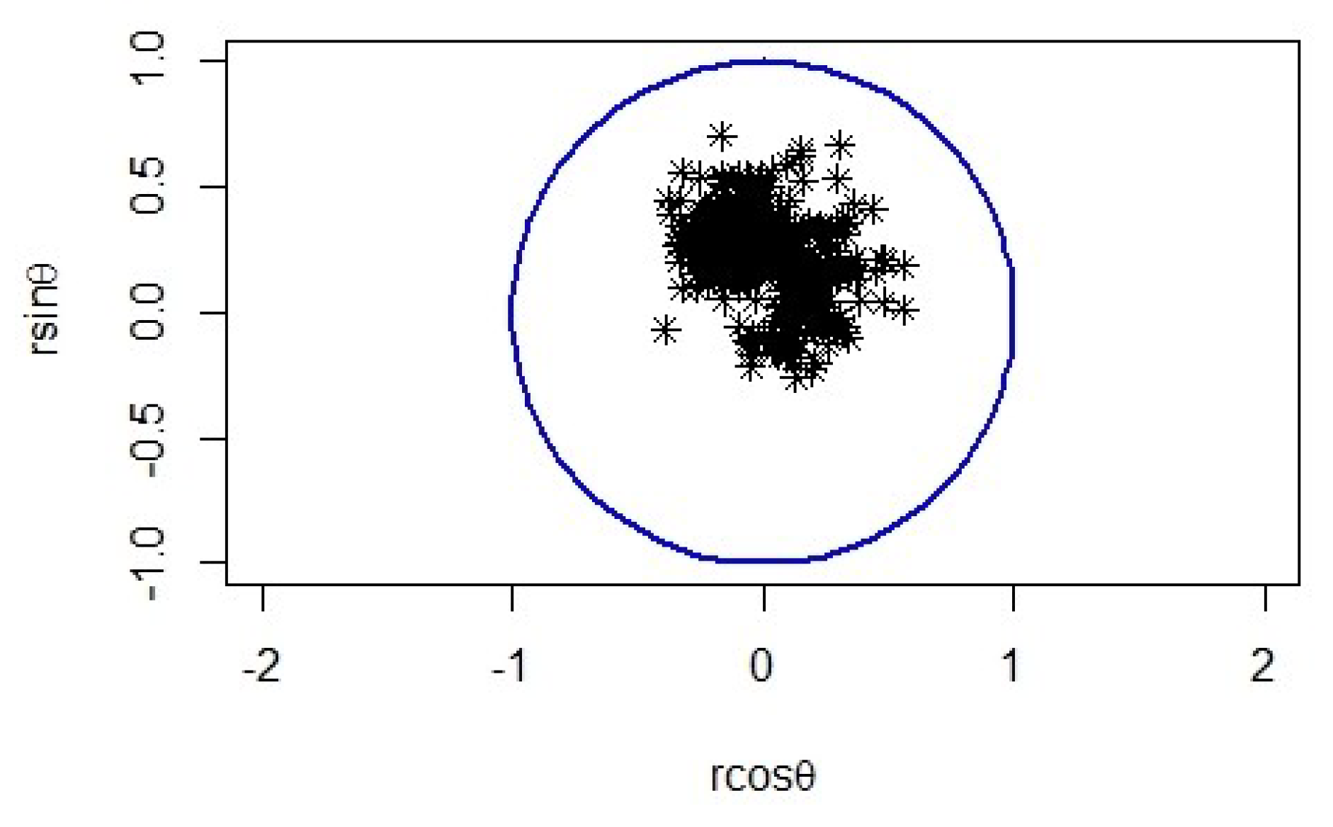
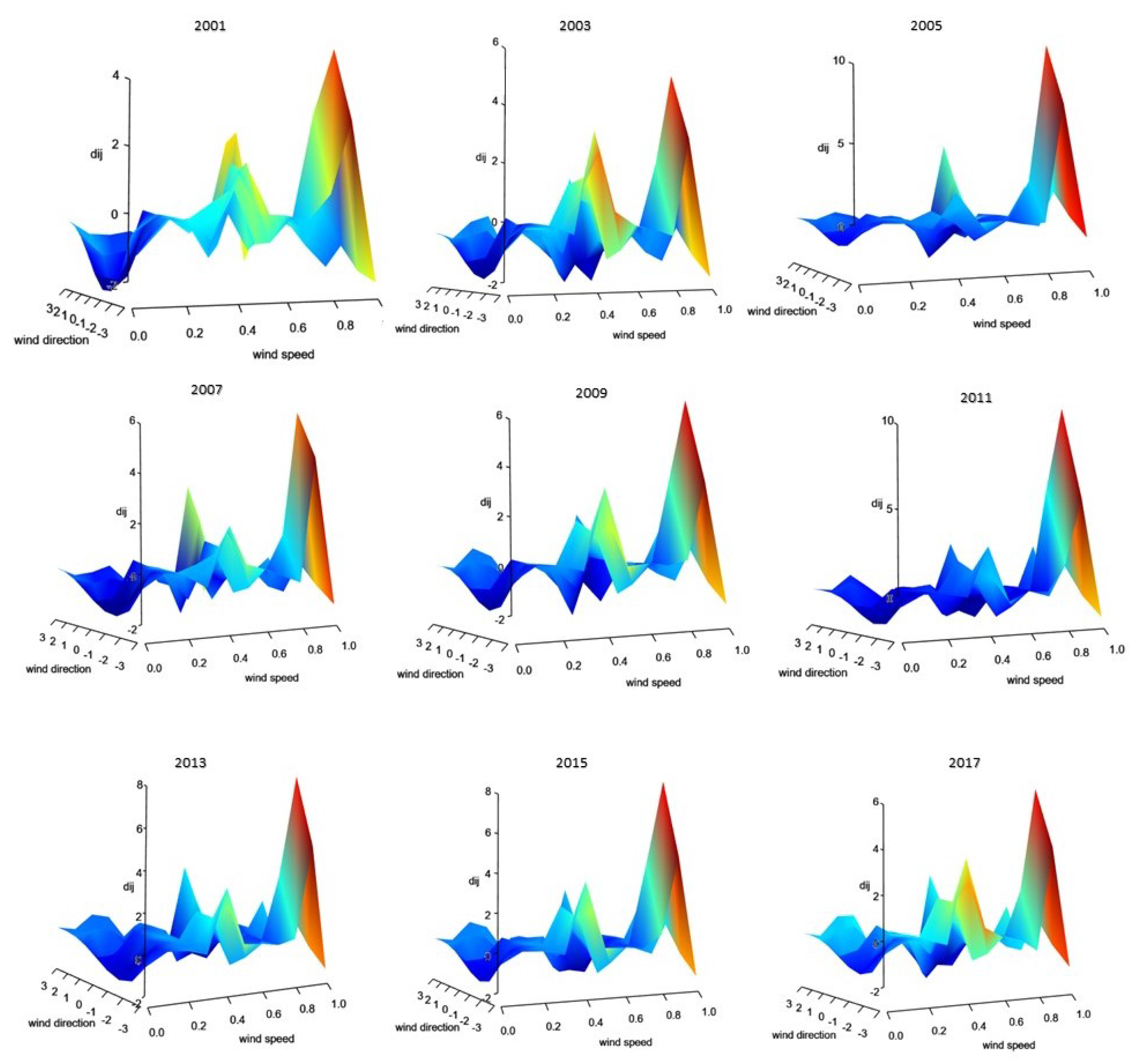
5. Illustrative Example: Marion Island Data

For evaluation of the models, in addition to the AIC and BIC, we considered the performance measure proposed by Mathisen, et al. [30], which is used to evaluate the fits of bivariate models. This method used for linear-circular models in [1] is the normalized deviation. This method is based on the normalized deviation, d i j between the observed number of data points, N i j ( o ) , falling in a cell and the expected number of points, n p i j ( e ) . The mathematical expression for the normalized deviation, d i j , is given by,
d i j = N i j ( o ) n p i j ( e ) σ i j ( e )
where σ i j ( e ) is the normalizing factor and the expected standard deviation for the number of data points falling in the cell. Values of normalized deviation close to zero indicate a good fit of the estimated models. The normalized deviation identify the areas in the ( r , θ ) plane where the model either underperforms or overperforms. The normalized deviation, d i j , is presented in Figure 13, for the model of best fit for each year according to the performance measures in Table 2. In Table 3, the range and median of the d i j for the models of best fit for each year is given. The values if d i j close to zero indicate a good fit of the model. Positive and negative values indicate underestimation and overestimation, respectively. In Table 4, a summary of the normalized deviations for the model of best fit for each year, based on Table 2, is provided. Figure 13 illustrates the normalized deviation plots for the model of best fit for each year.
In Table 2, the estimated values of the parameters of the models (Equations (4), (9), (15) and (19)) and their performances are summarized. The expressions for the maximum likelihood estimation for the parametric models are given in Appendix A.
The following inferences can be drawn from Table 2:
  • The general Möbius distribution (Equation (4)) performs fairly well most of the time and has the advantage of no distributional assumptions. However, it is worth noting that the selection of the bandwidth plays an important role in the directional analysis.
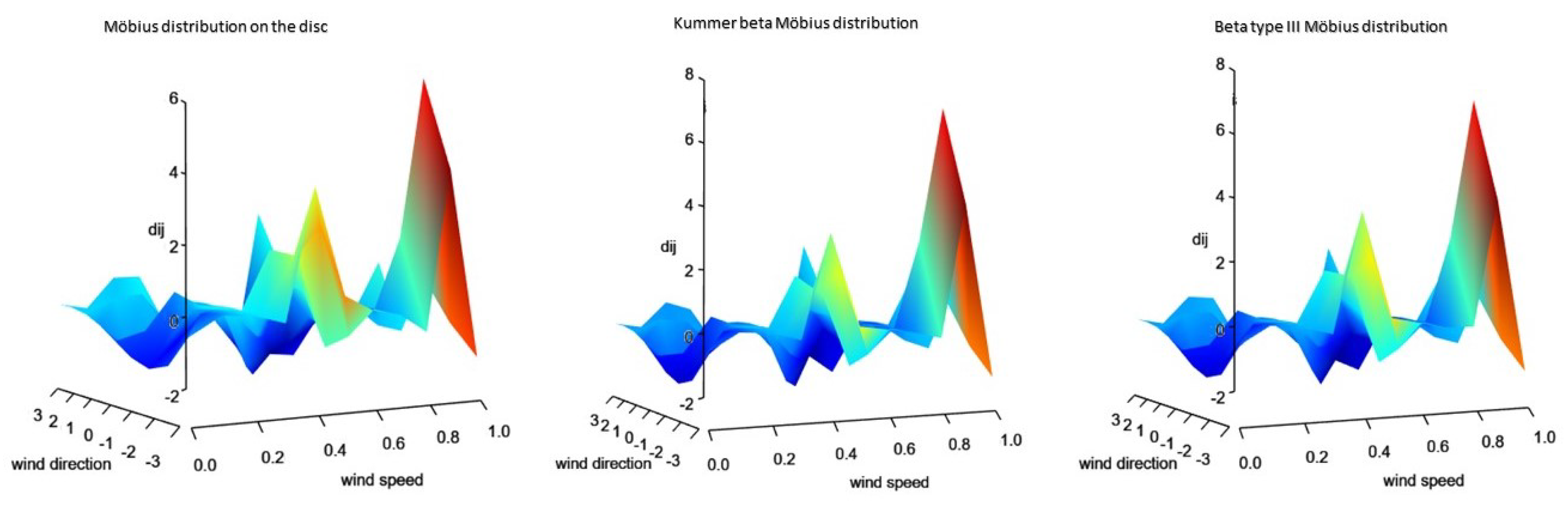
  • The Möbius distribution on the disc (Equation (9)) outperforms when there is unimodal behavior inherent in the data. This can be seen for the years 2003, 2005, 2007, 2013, 2015 and 2017.
  • The Beta type III Möbius distribution in Equation (19) outperforms when there is bimodal behavior inherent in the data. This can be seen for the years 2001, 2009 and 2011. It is also worth noting that the Beta type III Möbius distribution has the ability to model unimodality as well as bimodality. Hence, the performance of this model fairs well against the Möbius distribution on the disc.
  • It is interesting to note that the parameters introduced by the Möbius transformation, a and μ , have the same estimated values for the three parametric models. This highlights the influence of the Möbius transformation to the generator models.
For the year 2017, consider the estimated density function plot of the Möbius distribution on the disc in Equation (9) in Figure 14. In Table 4, the range and median of the normalized deviation for the proposed parametric models are compared and the plots of these normalized deviation are illustrated in Figure 15.

6. Conclusions

In this paper, we have developed a new general Möbius distribution class on the disc which has support on the unit disc that includes the well-known Möbius distribution on the disc proposed by [3] as a special case. This new class can assume either a semi-parametric or parametric form depending on the choice of the practitioner. This class of distributions is suitable when there exist bimodal patterns hidden in the data structure. Using the Marion Island climate data, model evaluation showed the performance of the different proposed models and the flexibility of this new class of distributions in capturing the bimodality and asymmetry present in the data. The Möbius transformation introduces asymmetry to the model in terms of off-centeredness as well as an orientation for the asymmetry. The ability of this new class to capture the bimodal behavior is a result of the generator function. One of the reviewers commented on that the low kurtosis values in Table 1 indicate a multimodal distribution. This needs further exploration. This work can be extended for modeling wind power density in wind energy analysis. To this end, it is sufficient to multiply the wind power density with the general Möbius density given by Equation (4) (for further details, refer to [12]).

Author Contributions

M.A., A.B. and P.N. equally contributed to the conceptualization, methodology, formal analysis, investigation, writing and project administration. P.N. contributed to the software and visualization. H.R. contributed to the description, availability and understanding of the data.

Funding

This work was based upon research supported in part by the National Research Foundation (NRF) of South Africa, Ref:CPRR160403161466 grant No. 105840 and SARChI Research Chair UID: 71199. Opinions expressed and conclusions arrived at in this study are those of the author and are not necessarily to be attributed to the NRF.

Acknowledgments

The authors would like to thank the anonymous reviewers for their insightful comments which led to an improvement of this paper. The authors would also like to thank Elsa de Jager from the National Climate Center, South African Weather Service for her assistance with the data description.

Conflicts of Interest

The authors declare no conflict of interest.

Appendix A

Appendix A.1. Möbius Distribution on This Disc

For the Möbius distribution on the disc, assuming that a 0 , the maximum likelihood estimators can be obtained by estimating the equations below derived from Equation (12),
0 = i = 1 n γ + 1 2 a r i sin θ i μ 1 2 a r i cos θ i μ + a 2 r i
0 = i = 1 n γ + 1 2 a r i 2 2 r i cos θ i μ 1 2 a r i cos θ i μ + a 2 r i
0 = i = 1 n ln 1 2 a r i cos θ i μ + a 2 r i i = 1 n ln 1 r i 2 n ln 1 a 2

Appendix A.2. Kummer Beta Möbius Distribution

For the Kummer beta Möbius distribution, assuming that a 0 , the maximum likelihood estimators can be obtained by estimating the equations below derived from Equation (17),
0 = i = 1 n [ a 2 2 a r i cos ( θ i μ ) + r i 2 ] [ 1 2 a r i cos ( θ i μ ) + a 2 r i 2 ]
0 = n Ψ ( β + γ ) n Ψ ( β ) + i = 1 n log [ a 2 2 a r i cos ( θ i μ ) + r i 2 ] i = 1 n log [ 1 2 a r i cos ( θ i μ ) + a 2 r i 2 ] n [ 1 F 1 ( 0 , 1 , 0 ) β , β + γ ; 1 + 1 F 1 ( 1 , 0 , 0 ) β , β + γ ; 1 ] 1 F 1 β , β + γ ; 1
0 = n Ψ ( β + γ ) n Ψ ( γ ) + n log [ 1 a 2 ] + i = 1 n log ( 1 r i 2 ) i = 1 n log [ 1 2 a r i cos ( θ i μ ) + a 2 r i 2 ] n [ 1 F 1 ( 0 , 1 , 0 ) β , β + γ ; 1 ] 1 F 1 β , β + γ ; 1
0 = i = 1 n 2 ( β 1 ) a r i sin ( μ θ i ) a 2 2 a r i cos ( θ i μ ) + r i 2 i = 1 n 2 ( γ + β ) a r i sin ( μ θ i ) 1 2 a r i cos ( θ i μ ) + a 2 r i 2 λ i = 1 n 2 a r i [ a 2 r i 2 + a 2 r i 2 ] sin ( μ θ i ) 1 2 a r i cos ( θ i μ ) + a 2 r i 2 2
0 = 2 a n ( γ + 1 ) ( 1 a 2 ) + i = 1 n ( β + 1 ) ( 2 a 2 r i cos ( θ i μ ) ) ( a 2 2 a r i cos ( θ i μ ) + r i 2 ) i = 1 n ( γ + β ) ( 2 a r i 2 2 r i cos ( θ i μ ) ) ( 1 2 a r i cos ( θ i μ ) + a 2 r i 2 ) λ i = 1 n 2 ( r i 2 1 ) a 2 r i cos ( θ i μ ) + r i cos ( θ i μ ) a 2 ( r i 2 + 1 ) 1 2 a r i cos ( θ i μ ) + a 2 r i 2 2
where Ψ ( · ) is the digamma function and 1 F 1 ( · ) · is the derivative of the confluent hypergeometric function.

Appendix A.3. Beta Type III Möbius Distribution

For the beta type III Möbius distribution, assuming that a 0 , the maximum likelihood estimators can be obtained by estimating the equations below derived from Equation (22),
0 = n log ( 2 ) + n Ψ ( β + γ ) n Ψ ( β ) + i = 1 n log [ a 2 2 a r i cos ( θ i μ ) + r i 2 ] i = 1 n log [ ( 1 + a 2 ) ( 1 + r 2 ) 4 a r i cos ( θ i μ ) ]
0 = n Ψ ( β + γ ) n Ψ ( γ ) + n log [ 1 a 2 ] + i = 1 n log ( 1 r i 2 ) i = 1 n log [ ( 1 + a 2 ) ( 1 + r 2 ) 4 a r i cos ( θ i μ ) ]
0 = i = 1 n 4 a r i ( β + γ ) sin ( θ i μ ) ( 1 + a 2 ) ( 1 + r 2 ) 4 a r i cos ( θ i μ ) i = 1 n 2 a r i ( β 1 ) sin ( θ i μ ) a 2 2 a r i cos ( θ i μ ) + r i 2
0 = i = 1 n ( β 1 ) ( 2 a 2 r i cos ( θ i μ ) ) a 2 2 a r i cos ( θ i μ ) + r i 2 2 n a ( γ + 1 ) 1 a 2 i = 1 n ( γ + β ) ( 2 a ( 1 + r i 2 ) 4 a r i cos ( θ i μ ) ) ( 1 + a 2 ) ( 1 + r 2 ) 4 a r i cos ( θ i μ )
where Ψ ( · ) is the digamma function.

References

  1. Soukissian, T.H.; Karathanasi, F.E. On the selection of bivariate parametric models for wind data. Appl. Energy 2017, 188, 280–304. [Google Scholar] [CrossRef]
  2. Jones, M.C. Marginal replacement in multivariate densities, with application to skewing spherically symmetric distributions. J. Multivar. Anal. 2002, 81, 85–99. [Google Scholar] [CrossRef]
  3. Jones, M.C. The Möbius distribution on the disc. Ann. Inst. Stat. Math. 2004, 56, 733–742. [Google Scholar] [CrossRef]
  4. Uesu, K.; Shimizu, K.; SenGupta, A. A possibly asymmetric multivariate generalization of the Möbius distribution for directional data. J. Multivar. Anal. 2015, 134, 146–162. [Google Scholar] [CrossRef]
  5. Abe, T.; Ley, C. A tractable, parsimonious and flexible model for cylindrical data, with applications. Econom. Stat. 2017, 4, 91–104. [Google Scholar] [CrossRef] [Green Version]
  6. Fernández-Durán, J.J. Models for circular–linear and circular–circular data constructed from circular distributions based on nonnegative trigonometric sums. Biometrics 2007, 63, 579–585. [Google Scholar] [CrossRef] [PubMed]
  7. Johnson, R.A.; Wehrly, T. Measures and models for angular correlation and angular-linear correlation. J. R. Stat. Soc. Ser. B Methodol. 1977, 39, 222–229. [Google Scholar] [CrossRef]
  8. Mardia, K.V.; Jupp, P.E. Directional Statistics; John Wiley & Sons: Chichester, UK, 2009; Volume 494. [Google Scholar]
  9. Ley, C.; Verdebout, T. Modern Directional Statistics; Chapman and Hall/CRC: New York, NY, USA, 2017. [Google Scholar]
  10. Pewsey, A.; Neuhäuser, M.; Ruxton, G.D. Circular Statistics in R; Oxford University Press: Oxford, UK, 2013. [Google Scholar]
  11. Basile, S.; Burlon, R.; Morales, F. Joint probability distributions for wind speed and direction. A case study in Sicily. In Proceedings of the 2015 International Conference on Renewable Energy Research and Applications (ICRERA), Palermo, Italy, 22–25 November 2015; pp. 1591–1596. [Google Scholar]
  12. Carta, J.A.; Ramirez, P.; Bueno, C. A joint probability density function of wind speed and direction for wind energy analysis. Energy Convers. Manag. 2008, 49, 1309–1320. [Google Scholar] [CrossRef]
  13. Han, Q.; Hao, Z.; Hu, T.; Chu, F. Non-parametric models for joint probabilistic distributions of wind speed and direction data. Renew. Energy 2018, 126, 1032–1042. [Google Scholar] [CrossRef] [Green Version]
  14. Zhang, J.; Chowdhury, S.; Messac, A.; Castillo, L. A multivariate and multimodal wind distribution model. Renew. Energy 2013, 51, 436–447. [Google Scholar] [CrossRef]
  15. Zhang, L.; Li, Q.; Guo, Y.; Yang, Z.; Zhang, L. An investigation of wind direction and speed in a featured wind farm using joint probability distribution methods. Sustainability 2018, 10, 4338. [Google Scholar] [CrossRef]
  16. Sanusi, N.; Zaharim, A.; Mat, S.; Sopian, K. Comparison of Univariate and Bivariate Parametric Model for Wind Energy Analysis. J. Adv. Res. Fluid Mech. Therm. Sci. 2018, 49, 1–10. [Google Scholar]
  17. Truswell, J.F. Marion Island, South Indian Ocean. Nature 1965, 205, 64. [Google Scholar] [CrossRef]
  18. Chown, S.; Froneman, P.W. (Eds.) The Prince Edward Islands: Land-Sea Interactions in a Changing Ecosystem; African Sun Media: Stellenbosch/Bloemfontein, South Africa, 2008. [Google Scholar]
  19. Schulze, B.R. The climate of Marion Island. In Marion and Prince Edward Island, Report on the South African Biological and Geological Expedition 1965–1966; Van Zinderen Bakke, E.M., Sr., Winterbotton, J.M., Dyer, R.A., Eds.; A.A. Balkema: Cape Town, South Africa, 1971; pp. 16–31. [Google Scholar]
  20. Le Roux, P.C. Azorella selago (Apiaceae) as a Model for Examining Climate Change Effects in the Sub-Antarctic. Ph.D. Thesis, Stellenbosch University, Stellenbosch, South Africa, 2004. [Google Scholar]
  21. Rouault, M.; Mélice, J.L.; Reason, C.J.; Lutjeharms, J.R. Climate variability at Marion Island, southern ocean, since 1960. J. Geophys. Res. Oceans 2005. [Google Scholar] [CrossRef]
  22. Rudin, W. Real and Complex Analysis, 3rd ed.; McGraw-Hill: New York, NY, USA, 1987; pp. 249–250. [Google Scholar]
  23. Krantz, S.G. Handbook of Complex Analysis; Birkhäuser: Basel, Switzerland, 1999. [Google Scholar]
  24. Kato, S.; Jones, M.C. A family of distributions on the circle with links to, and applications arising from, Möbius transformation. J. Am. Stat. Assoc. 2010, 105, 249–262. [Google Scholar] [CrossRef]
  25. Minh, D.L.; Farnum, N.R. Using bilinear transformations to induce probability distributions. Commun. Stat. Theory Methods 2003, 32, 1–9. [Google Scholar] [CrossRef]
  26. Johnson, M.E. Multivariate Statistical Simulation; Wiley: New York, NY, USA, 1987. [Google Scholar]
  27. Nagar, D.K.; Gupta, A.K. Matrix-variate Kummer-beta distribution. J. Aust. Math. Soc. 2002, 73, 11–26. [Google Scholar] [CrossRef]
  28. Cardeno, L.; Nagar, D.K.; Sánchez, L.E. Beta type 3 distribution and its multivariate generalization. Tamsui Oxf. J. Math. Sci. 2005, 21, 225–242. [Google Scholar]
  29. Abramowitz, M.; Stegun, I.A. Handbook of Mathematical Functions: With Formulas, Graphs, and Mathematical Tables; Courier Corporation: Mineola, NY, USA, 1965; Volume 55. [Google Scholar]
  30. Mathisen, J.; Bitner-Gregersen, E. Joint distributions for significant wave height and wave zero-up-crossing period. Appl. Ocean Res. 1990, 12, 93–103. [Google Scholar] [CrossRef]
Figure 1. Images of the location and weather station of Marion Island. (a) An image of the location of Marion Island. (Image obtained from https://www.environment.gov.za/mediarelease/princeedwardislands_declaredmarineprotectedarea on 9 February 2019). (b) An image of the Marion Island weather station. (Image obtained from http://blogs.sun.ac.za/antarcticlegacy/about-2/marion-station on 9 February 2019).
Symmetry 11 01030 g001
Figure 2. A rose diagram of the wind direction (left); and histogram of the wind speed (right) from the data observed at Marion Island for 2017.
Symmetry 11 01030 g002
Figure 3. A scatter plot of the wind speed and wind direction data from Marion Island for 2017.
Symmetry 11 01030 g003
Figure 4. The density function and contour plot of the bivariate Pearson Type II distribution in Equation (8) for γ = 5 .
Symmetry 11 01030 g004
Figure 5. The marginal density function of the bivariate Pearson Type II distribution in Equation (8) for γ = 0.5 , 1 , 3 from left to right.
Symmetry 11 01030 g005
Figure 6. Density function and contour plots of the Möbius distribution on the disc, Equation (10), for varying parameter values.
Symmetry 11 01030 g006
Figure 7. The density function and contour plot of the bivariate Kummer beta distribution in Equation (12) for γ = 3 , β = 2 and λ = 0.5 .
Symmetry 11 01030 g007
Figure 8. The marginal density function plot of the bivariate Kummer beta distribution in Equation (12) for γ = 2 , 2 , 2 , β = 3 , 1 , 3 and λ = 1 , 1 , 4 from left to right.
Symmetry 11 01030 g008
Figure 9. Density function and contour plots of the Kummer beta Möbius distribution, (16), for varying parameter values.
Symmetry 11 01030 g009aSymmetry 11 01030 g009b
Figure 10. The density function and contour plot of the bivariate Beta type III distribution in Equation (17) for γ = 3 and β = 2 .
Symmetry 11 01030 g010
Figure 11. The marginal density function plot of the bivariate Beta type III distribution in Equation (17) for γ = 2 , 0.5 , 2 and β = 3 , 3 , 1 . from left to right.
Symmetry 11 01030 g011
Figure 12. Density function plot and contour plots of beta type III Möbius distribution, (20), for varying parameter values.
Symmetry 11 01030 g012aSymmetry 11 01030 g012b
Figure 13. The normalized deviation for the model of best fit for each year.
Symmetry 11 01030 g013
Figure 14. The density function plot and contour plot of the Möbius distribution on the disc (9) for the estimated parameter values a ^ = 0.22 , μ ^ = 1.59 and γ ^ = 12.14 .
Symmetry 11 01030 g014
Figure 15. The normalized deviation for the parametric models for 2017.
Symmetry 11 01030 g015
Table 1. Circular statistics for the wind direction at Marion Island for nine years.
Year r ¯ θ ¯ V Θ ν Θ δ ^ s ^ k ^
20010.59−1.380.400.891.14−1.60−3.38
20030.58−1.430.410.901.18−1.67−3.02
20050.58−1.520.410.911.21−1.70−2.84
20070.481.480.521.022.20−0.84−1.59
20090.57−1.560.430.931.35−1.55−2.41
20110.571.560.430.931.33−1.58−2.45
20130.561.530.440.941.39−1.56−2.24
20150.561.520.430.931.36−1.58−2.32
20170.531.450.470.971.71−1.11−2.04
Table 2. Results from fitting the proposed distributions to the Marion Island data.
EstimatesPerformance
Model a ^ μ ^ γ ^ β ^ λ ^ Log-LikelihoodAICBIC
Year 2001
 General Möbius distribution (h = 0.0109)0.31.88---−295.68595.37602.85
 Möbius distribution on disc0.171.959.46--−293.38592.75603.97
 Kummer beta0.161.972.661.4212.52−286.85583.71602.41
 Beta type III0.151.936.891.40-−286.87581.74596.69
Year 2003
 General Möbius distribution (h = 0.0088)0.41.88---−281.06566.11573.91
 Möbius distribution on disc0.211.7411.55--−276.29558.57570.27
 Kummer beta0.211.7611.861.151.86−274.16558.31577.81
 Beta type III0.211.787.411.24-−275.01558.01573.61
Year 2005
 General Möbius distribution (h = 0.0096)0.31.26---−277.18558.36566.08
 Möbius distribution on disc0.201.2811.39--−271.14548.27559.85
 Kummer beta0.201.279.131.033.25−271.39552.77572.06
 Beta type III0.201.286.451.04-−272.18552.36567.79
Year 2007
 General Möbius distribution (h = 0.0107)0.21.26---−354.05712.10719.89
 Möbius distribution on disc0.181.599.33--−349.50705.01716.70
 Kummer beta0.181.601.181.1711.69−346.84703.68723.17
 Beta type III0.171.616.221.23-−347.00702.01717.59
Year 2009
 General Möbius distribution (h = 0.0079)0.31.26---−282.38568.77576.57
 Möbius distribution on disc0.191.5911.91--−280.42566.83578.53
 Kummer beta0.191.617.691.349.16−274.04558.08577.58
 Beta type III0.201.628.671.38-−274.31556.63572.23
Year 2011
 General Möbius distribution (h = 0.0078)0.21.88---−277.24558.48566.27
 Möbius distribution on disc0.181.5113.54--−275.09556.19567.88
 Kummer beta0.181.4714.841.241.88−270.37550.74570.22
 Beta type III0.181.489.361.29-−270.53549.06564.65
Year 2013
 General Möbius distribution (h = 0.0089)0.31.88---−258.28520.56528.32
 Möbius distribution on disc0.191.5612.55--−251.43508.86520.51
 Kummer beta0.191.5510.221.194.99−249.76509.52528.92
 Beta type III0.201.568.271.25-−250.50509.00524.52
Year 2015
 General Möbius distribution (h = 0.0073)0.21.88---−261.57527.15534.95
 Möbius distribution on disc0.191.5913.79--−253.29512.58524.27
 Kummer beta0.191.5413.281.040.61−253.79517.57537.06
 Beta type III0.191.568.151.12-−253.77515.55531.14
Year 2017
 General Möbius distribution (h = 0.00818)0.21.26---−261.99527.98535.77
 Möbius distribution on disc0.221.5912.14--−258.51523.01534.69
 Kummer beta0.211.5711.591.152.44−257.25524.50543.97
 Beta type III0.211.617.561.15-−257.91523.82539.39
Table 3. Normalized deviation ranges for model of best fit for each year.
YearBest Fit ModelRangeMedian
2001Beta type III Möbius (19)(−2.651791; 5.920593)−0.1554433
2003Möbius distribution on the disc (9)(−2.312973; 6.288503)−0.147436
2005Möbius distribution on the disc (9)(−3.453434; 12.743586)−0.1662767
2007Möbius distribution on the disc (9)(−2.610813; 7.522888)−0.3437355
2009Beta type III Möbius (19)(−3.000686; 7.984593)−0.05206841
2011Beta type III Möbius (19)(−2.482695; 12.845301)−0.08473761
2013Möbius distribution on the disc (9)(−2.404983; 9.312558)−0.05009261
2015Möbius distribution on the disc (9)(−2.516891; 9.782227)−0.03193083
Table 4. Normalized deviation ranges for the parametric models for 2017.
ModelRangeMedian
Möbius distribution on disc (9)(−2.933306; 7.795678)−0.07912035
Kummer beta Möbius (15)(−2.859249; 8.231555)−0.06817048
Beta type III Möbius (19)(−2.964023 8.259554)−0.100007

