Abstract
In this work, we deal with a kinetic model of cell movement that takes into consideration the structure of the extracellular matrix, considering cell membrane reactions, haptotaxis, and chemotaxis, which plays a key role in a number of biological processes such as wound healing and tumor cell invasion. The modeling is performed at a microscopic scale, and then, a scaling limit is performed to derive the macroscopic model. We run some selected numerical experiments aimed at understanding cell movement and adhesion under certain documented situations, and we measure the alignment of the cells and compare it with the pathways determined by the extracellular matrix by introducing new alignment operators.
1. Introduction
Studying and understanding cell movement is crucial in biological sciences and medicine, since it is essential to a variety of biological processes such as morphogenesis, wound healing, cancer metastasis, and immune response, among others [1]. Haptotaxis is understood as the movement of the cells due to interactions with the substances that form the extracellular matrix (ECM), and it is influenced by its structure. Depending on the cell type, its size, and if the migration is individual or collective, we can find different types of haptotactic movements [2,3]. Haptotaxis occurs either due to the presence of an oriented compound on the ECM, like a filament or a proteic fiber, or by a difference in the concentration of certain chemical compounds that stick to the ECM and promote binding of cells. The latter might be seen as a similar mechanism to chemotaxis; however, chemotaxis should not be seen as a special case of haptotaxis [4]. One of the structures that appears when studying the haptotactic movement of cells is the integrins, cell membrane adhesion proteins that bind with the substances on the ECM [5,6].
On the other hand, chemotaxis is a process by which cells change their state of movement reacting to the presence of a certain free chemical compound in the surrounding media of the cell population. Usually, cells are affected by both phenomena simultaneously, even it is possible to be caused by the same substance on different states. This is the case of thrombospondin 1, forcing both haptotaxis and chemotaxis on the movement of melanoma cells [7,8,9].
Both processes, chemotaxis and haptotaxis, constitute directional mobilities of cells whose driving forces are gradients: for haptotaxis, a gradient of cellular adhesion sites, while for chemotaxis, a chemical concentration gradient in a soluble fluid. These gradients are naturally present in the ECM of the body during processes such as angiogenesis or artificially-induced in biomaterials where gradients are established by altering the concentration of adhesion sites on a polymer substrate.
The binding of cells to the ECM and the different processes that modify the state of the integrins have been studied from a mathematical point of view. We refer the reader to [10] for some models focused on cell reactions involving these compounds. In [11], these reactions were incorporated into a kinetic model for cell motility, adding the concentration of integrins as a new microscopic variable, taking the main role in promoting the movement of the cellular population.
In the literature, chemotaxis has received much more attention than haptotaxis, starting with the classical model due to Patlak [12], and Keller and Segel in the 1970s [13]. The mathematical properties of this classical model for chemotaxis, in particular the blow-up of the solutions for finite time, have led to the development of new ways of studying chemotaxis from a mathematical point of view, many of them modifying the aforesaid model. The survey by Hillen and Painter [14] collected several different variations of this classical model, and they incorporated new mathematical terms modeling biological phenomena, such as nonlinear diffusion, non-constant sensibility to the chemoattractant, and control of the population by direct or indirect ways, among others. These models can also be deduced from a microscopic point of view by using the tools of hydrodynamical limits [15,16].
More recent results on this challenging topic were reviewed in the surveys [17,18], while some recent achievements have enlightened the role of anomalous diffusion [19,20] and of the environment where the dynamics develops [21]. Indeed, our paper considers models in the complex environment constituted by the ECM, where cells move.
On the other hand, the development of mathematical models studying haptotaxis is relatively recent. Starting with the first model of Oster et al. in the early 1980s [22], early models for haptotactic movement were proposed as a particular case of chemotaxis with a non-diffusing signal. Later, in [23], the authors introduced both the adhesion of cells to the ECM, as well as the cell-membrane integrins, responsible for the aforementioned adhesion and promoters of cell migration. Recent works [11,24] have two important differences from the previous ones: first, the modeling was done through a kinetic approach to haptotaxis; second, the directionality of the structural compounds of the ECM, and not the gradient of said compounds, took the main role in cell motility.
There exists a wide literature related to the mathematical modeling of cell motility, which due to the biological nature of the phenomena, involves an appreciable complexity. One of the most visited topics is the modeling of the invasion of healthy tissues by tumors. In particular, we remark about the contribution by Chaplain et al. [25], where a complete model containing haptotaxis due to the ECM, chemotaxis due to different chemical compounds in the surrounding media, and interactions between all the involved cells was deduced for the cancer cell invasion of a tissue. In this line, many more rigorous and numerical approaches have been tackled (see [23,24,26,27,28] among others) by using kinetic and/or macroscopic models, each of them with its own mathematical complexity.
It is worth mentioning that the mathematical modeling of biological phenomena and, in particular, of the dynamics of multicellular systems has recently taken advantage of the framework delivered by the so-called Kinetic Theory of Active Particles (KTAP) [29]. The main difference of the KTAP approach with respect to the classical kinetic theory to model living systems is that the microscopic state of the interacting entities, which are called active particles, includes, in addition to mechanical variables, another variable called activity, which models biological functions specific for each system under consideration. This is the approach used in the present paper, by highlighting that the activity variable allows us, in contrast with other approaches, to consider several microscopic biological variables as independent variables, and not as unknowns, whose dynamics is well defined, obtaining an important reduction of the complexity of the final model.
Some specific tools of the KTAP approach have so far been used in many other applications. For instance, competition between tumor and immune cells [30] and social dynamics [31,32], crowd dynamics [17,18,33,34,35,36], and swarming [37]. Thus, the contents of this paper may be useful for the modeling of other phenomena in life sciences. Notice that the modeling of these specific systems needs a deep understanding of the interactions between living entities, as in the case of cell dynamics, where the “living behavior” belongs to the specific functions expressed by cells. Mathematical models require the application of computational methods appropriate for capturing the specific features of multi-agent systems. Monte Carlo particle methods have shown the ability to handle this challenging problem of numerical analysis [38].
Finally, let us mention some specific applications on the derivation of macroscopic equations from the underlying description at the microscopic scale delivered by kinetic theory models. Various types of regular and singular perturbation methods have been applied for different types of models, as examples in vehicular traffic [34], as well as in the dynamics of cells [20,21,39]. The unified approach of a method inspired to the Hilbert problem was developed in [40], while a general reference was given by [41].
The paper is organized as follows. Section 2 presents the kinetic model for the movement of a cell population whose physical-biological properties were described in [42,43] and performs the hyperbolic scaling for the underlying description at the micro- and meso-scopic scales. Section 3 is devoted to the numerical scheme, and three case-studies are proposed and analyzed with special insight into a measure of alignment for the adaptation of cells to the ECM. Finally, Section 4 presents the conclusions and some research perspectives.
2. Description of the Model
This section is devoted to the description of the model presented in [43] and the hyperbolic scaling. The model describes the movement of a cell population in and the evolution of two chemical compounds, each one related to one of the processes described before: an oriented protein fiber, denoted by , where represents its orientation, and a degenerated chemical , responsible for chemotaxis. The density of proteic fibers at time t and position x is denoted by :
We describe the cell population by means of a distribution function depending on time t, space x, velocity v, and activity y (which will be described below), verifying the following equation deduced in [42],
where the right-hand side models the cell mobility by way of velocity changes and the y-divergence term is related to the cell membrane reactions. Concretely,
- the term , modeling haptotaxis, is:
- the turning operator models random changes in velocity,
- and the chemotactic term, , reads:
Here, , and are the interaction frequencies, , T and K are the interaction kernels, and are nonnegative weight functions satisfying . V is the domain of velocities, which is given by the velocities verifying .
In order to define the activity y and the cell membrane reaction terms, we need to recover the law of mass action of the reactions produced at the cell membrane involving the two chemicals in the ECM and the receptors on the cell,
where R stands for the free enzyme on the cell surface and and represent the respective complexes once the enzyme binds the ECM chemical. Then, y is defined as the two-component vector of microscopic concentrations of the two cell-membrane compounds and , respectively. It is defined in the set:
where represents the maximum concentration of receptors on the cell surface. The function G is given by the expression:
whose rows represent the equations associated with (2).
Finally, we introduce the macroscopic equations for the free chemicals Q and L in the ECM:
and:
The Hyperbolic Scaling
We have so far referred to macroscopic and microscopic models. However, they are not independent of each other, since they are two different ways of viewing the same reality. If we face the same real situation, whose nature requires different scales, we must describe it by combining models of the two types, which should be related in some way. This is the underlying concept of multiscale modeling: modeling the same real situation with different scales, and their relationship. The relationship between the different scales is given by scaling limit: broadly speaking, it is performed by “zooming out” the window through which we observe a phenomenon, and by transforming a microscopic model into a macroscopic model.
In this subsection, we perform the calculations leading to the nondimensionalization and scaling of the system(1)–(3)–(4) [43].
In the following, the interaction frequencies , , and are considered to be constant (otherwise, the scaling does not make sense). First of all, we define the dimensionless (“hat”) variables:
where and are typical quantities of their respective variables. The new variables are defined in the sets:
Our system then becomes:
We impose first the normalization restrictions and . The hyperbolic scaling corresponds to the choice:
i.e., the turning time is very small compared to the typical time .
There are three other phenomena (cell membrane reactions, haptotaxis, and chemotaxis) to consider. We rescale the corresponding terms, assuming also that their frequencies are small compared to the turning frequency . More precisely, we choose the following relations:
where , .
To scale the other two equations, we recall that they are actually macroscopic, so they will preserve their form. This is why we only define the scaled dimensionless constants involved:
Skipping the “hat” for the dimensionless variables, our system becomes:
for the cell population, where:
and:
for the chemicals, where:
and . In order to close the macroscopic system that will appear, we choose the turning operator:
with . If we study the equations verified by the moments of ,
we obtain the following equations:
Here, is the pressure tensor, and the matrix and the vector are respectively given by:
Then, we make on (5) to deduce that the limiting distribution function has to be on the kernel of the turning operator, i.e., , and then, we assume that the solutions are small perturbations of it, , hence a Hilbert expansion of around . Inserting the explicit form of (see [43] for details) into (12)–(13)–(14), we formally obtain the following macroscopic equations:
Here, the macroscopic integral operators are defined as:
where the macroscopic functions that appear are given by:
Finally, the limiting equations for Q and L can be written as follows:
where .
We remark here that this obtained fluid-type macroscopic model (15) contains an equation, the third one, which relates in an algebraic direct way (and not by a differential equation, thus reducing the usual complexity of these models) the macroscopic density of moving cells with the two densities of ECM compounds, and L, associated with the haptotaxis and chemotaxis phenomena. A simple first application of this fact is described in Section 3.2, where a comparison of simulations at micro- and macro-scales is stated.
3. The Numerical Scheme
This section is devoted to some numerical experiments designed to test in silico the accuracy of the model and to predict cell behavior. We were mainly interested in the study of the spreading of a tumor population through a formed living structure. Depending on the cancer type and the host tissue, this invasion can occur in either an individual or collective manner (see [24]) and can give rise to several type of patterns. In this sense, there is a huge literature of mathematical models for cancer invasion (see [44]), which denotes the complexity and heterogeneity of these phenomena. Therefore, we studied several simple situations, by using the presented model, which can reproduce many of these interactions between the moving cells and the surrounding ECM, and will try to measure the accuracy of the cells in adapting their invasion by following the orientation of the ECM fiber.
Simulations were obtained by solving the system (1)–(3)–(4), endowed with initial conditions and for the cell population and the ECM, respectively, which will be described for each different situation. The system was set in a spatially-square domain (thus ), for velocities (fixed modulus s), and y supported in the set Y defined on (11). We considered periodic boundary conditions in x and zero-flux in the activity y. These sets were discretized using a rectangular grid for position and activity and choosing eight directions in .
The numerical solution of the system was obtained by using a splitting method. The idea behind this approach was to write, at least formally, the overall evolution operator as the sum of evolution operators for each term in the model, then to pick an appropriate scheme for each term and attach the pieces together. We refer the reader to [45] for more details on the technique of splitting for numerically solving partial differential equations.
Therefore, the system was split into the following subequations:
The system was separated into three different blocks, namely: the transport equation, the integral operators that rules the changes of velocities, and the two equations for the ECM. The order in which these blocks are solved is a key point in the modeling (therefore, in the numerical scheme): a different order could give a different behavior of the system. Then, the system was solved in the same order as the blocks have been presented, i.e.:
- First, we solved the transport term, related to the evolution of position and cell activity;
- Second, the integral operators were treated, thus giving the new velocities;
- Finally, we dealt with the equations for the ECM compounds, Q and L.
We proceed to describe the techniques used in each step.
The first part of the splitting solved the modifications on position and activity of the cells. We split it again, obtaining two terms: the first one, related to the pure transport part of the equation, was solved using a finite volume scheme; the second term, , obtained from the divergence of the activity, was in fact an ODE in time, where the other variables acted as parameters, so it was directly solved using a first order Euler method to go forward in time (i.e., explicit Euler).
In the second step of the splitting, for each of the three different integral operators, we had to determine the interaction kernels. In the numerical schemes for kinetic equations, this is equivalent to building a certain table (table of games) for each one of them, containing the different transition probabilities. These will describe how, from an initial velocity coming from the previous step of the simulation, we obtained a new exit orientation as a weighted sum of the candidates proposed for each operator.
The turning operator is simpler: the candidate orientation is given by either a uniform distribution or by a normal distribution in centered on the initial orientation .
Turning is weighted with chemotaxis by , so this will be the next to be described. For each point, we calculated the gradient of the chemoattractant, . Next, given the entry velocity , we calculated the direction of the vector , named . Here, K was associated with the sensitivity to the signal. Then, the table of games was given by a normal distribution centered on with variance .
The joint table was then built, where each value was the weighted sum (by ) of each correspondent value.
For the haptotactic phenomena, the candidate orientation, , was given in each position by the mean orientation of the fibers on the said position:
In order to take this velocity to the grid of possible velocities, and to build the table, we applied a normal distribution centered on with (small) variance .
Once we had both tables, we weighed them accordingly (giving more importance to haptotaxis), and we constructed the final table of games. To avoid big leaps in the changes of velocities, the new velocity was taken as the nearest orientation from the initial velocity, in the direction of the orientation given by the calculated game. Finally, the new orientation was chosen between the candidate velocity, previously calculated, and the velocity the cell already had, representing the “decision” of a cell to follow the dictated movement.
It remains to solve the equations for both chemical compounds, Q and L. The equation for Q is essentially an ODE in time (the dependence with x and is parametric). To solve it, for each position x and orientation , we numerically computed the three integrals that appeared on the right-hand side and used a first order Euler method to advance in time. For L, the first step was to compute the diffusion term. To do that, first, was regularized using an implemented MATLAB function, SmoothN, to avoid problems with subsequent steps; then, we calculated using the implemented function Del2, which computed the discrete Laplacian. Then, the dependence of the equation with respect to the spatial variable could be considered parametrical, so we solved the equation as an ODE in time: numerical computation of the integral terms, and used the explicit Euler to obtain the next iteration.
From the nondimensionalization performed in the previous section, it is worth noticing that, in fact, we had two different concentrations: one, the cell-membrane concentrations of the bounded compounds (), whose units were (number of whatever)/(“area” units); and the concentrations of the free compounds (), with units (number of whatever)/(“volume” units). Therefore, a well-designed numerical scheme must take this into consideration and modify the constants in a suitable way. We modified the cell-membrane constants, now in units of (number of whatever)/(“volume”), by way of calculating the ratio between the area and the volume of a cell, and we converted the concentrations accordingly. Then,
which has units of concentration in a “volume”. We are in dimension , then the “area” reads for the length unit in the cell-membrane, and the “volume” is an area. If, for example, we assume that cells have the shape of a circle of diameter d, the conversion factor reads:
In the following, we will incorporate these computations into the numerical computations, and then, both concentrations will be equally named where there is no possibility of misunderstanding.
3.1. Adaptation of Cells to the ECM: A Measure of Alignment
In this subsection, we introduce some alignment functions in order to measure and understand the degradation of the ECM and the adaptation of cells to its structure. We focus our 2D simulations on three situations, as suggested in [24]: straight line-oriented fiber (following the axis), radially-oriented fiber, and randomly-oriented fiber. In order to measure the orientation of the fiber and the final adaptation of the invading cells to this tissue, we can define, for any fixed orientation , the normalized operators: the fiber alignment function:
which measures, at any time t and any perpendicular position a, the mean orientation of the fiber along the straight line (note that , its maximum value, fits exactly the -orientation). Analogously, we can define the cell alignment function:
which measures, at any time t and any perpendicular position a, the relative density of cells being on the straight line and moving with velocity on the same straight line, i.e., the ratio of cells that “follow” the orientation of the ECM fiber.
For the radial case, we can decompose the position as and use the following radial fiber alignment function,
in order to measure the radial orientation of the fiber, a standing for the selected angle. In this case, the relative density of cells following the radial pattern can be given by:
3.2. Comparison between the Behavior of Activity and Its Limiting Counterpart
When we obtained the macroscopic limiting system in the previous section, we defined the activity moment of the solution , which can be interpreted as the two-component vector of the mean concentration on the cells of the two cell-membrane compounds related to the binding with the chemicals of the ECM. The evolution of this quantity can be related to the modifications on the ECM, and the movement of fibers and L due to being carried by the cells.
We checked that, in the limit (15), could be obtained from a linear system of equations that yields the following explicit expression (related to the equilibrium state of the cell-membrane reactions):
Then, we can compute , both via:
and the previous quantity. The comparison between both quantities can measure how far the different cell-membrane reactions are from the equilibrium state.
Now, we will describe each simulation, giving the initial data for the cell population and the ECM fibers . Furthermore, each numerical experiment assumed that initially , which represents the fact that there was no chemoattractant in the environment, and it only appeared because of the degradation of the fibers Q. For each simulation, we will explain its motivation and the expected behavior, and we will interpret the results. The constants used in the numerical scheme are given in Table 1.

Table 1.
Constants used in the numerical scheme.
3.3. First Example: Fully-Oriented ECM
We start with the first proposed scenario: initially, we had a fully-oriented ECM, in the direction of the axis, distributed following parallel (regularized) strips in said direction, creating “pathways” of oriented fiber. Therefore, at time , the alignment function of the fiber with respect to the vertical direction was equal to one, (at least where there was some fiber), and zero in any other direction, as shown in Figure 1.
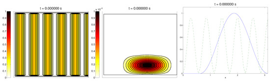
Figure 1.
First example: initial conditions for the ECM fibers (oriented in the direction (0,1)), cell population, and the alignment functions (dotted) and (dashed).
For the cell population, we aimed to represent the cell invasion on a living tissue (tumoral invasion) or the creation of new structures following previously-established signals and pathways (growth of neural networks). Thus, we chose an initial cell population concentrated near the border and regularized, with velocities randomly chosen such that , and initial activities and were small (around ). Then, the alignment of the cells with respect to the direction was not one on every horizontal position a.
Ideally, this is better represented by a fully-concentrated population in the line with completely random velocities. However, some regularizations and restrictions had to be made, in order to be able to perform the numerical scheme.
In this situation, we expected that would come closer to one as time went on, meaning the alignment of the cells with the ECM; meanwhile, should be kept close to one, as any change on the relative orientation should arise from new Q incorporated by means of the cell-membrane reactions. Furthermore, the cells should move upwards, more likely following the stripes of oriented fibers, and chemical L should appear from the degradation of the ECM. Finally, we expected that the cell-membrane reactions would come closer to the equilibrium state, as determined by (16). The numerical experiments confirmed our expectations: we saw that the cell population approached the strips of Q and, as they reached these strips, aligned with them, following their direction. This behavior is explicit in the joint graphic for both alignment functions (Figure 2), due to the coincidence of the peaks of and . In these simulations, we did not see significant ECM degradation due to the action of cells. In conclusion, we numerically confirmed that, in this example, haptotaxis dominated chemotaxis when leading cellular migration.
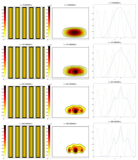
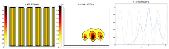
Figure 2.
Graph representing the evolution of the ECM (left), cell population (center), and the alignment functions (dotted) and (dashed) for the first example.
3.4. Second Example: Radially-Oriented ECM
In this case study, we started with a radially-oriented distribution of proteic fibers, centered at a fixed point of the grid, which for simplicity was chosen as , distributed following four straight lines equally distributed from the origin. This choice for the origin is consistent with the previous definitions of the radial orientation measures. Furthermore, the origin point would be at the center of the domain. Then, the initial radial fiber alignment function was equal to one on the four values of the arc a corresponding to the straight lines (and zero, if there was no Q compound there); see Figure 3.
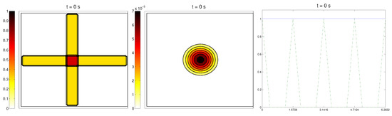
Figure 3.
Second example: initial conditions for the ECM fibers, cell population, and the alignment functions (dotted) and (dashed).
For the cell distribution, this situation would resemble in vitro experiments for development and invasion of a growing bacterial population. Then, was chosen as a (regularized) cut-off function of a small circular domain centered at the origin , the same point from where the fiber originated. The initial velocities of cells were randomly chosen in . Then, the initial radial alignment operator for the cells was a random distribution, taking values between zero and one. As in the previous example, the initial activities were set small.
In this situation, we expected the same behavior as in the previous example, now with the radial alignment operators and , instead of the fixed direction ones, and , respectively. In short, should come closer to one, meaning that cells follow the orientation ruled by the ECM, should decrease slightly, L should appear from the degradation of the matrix, and the activity should approach its equilibrium state.
Simulations partially confirmed our expectations: cells concentrate at those regions where the Q compound is present and align to its orientation, following the movement along the trail, as we can see in Figure 4. We also see, in the graphic of the alignment functions and , that the peaks of both functions are close to each other, which correspond to the influence of the other two modeled phenomena, chemotaxis and random motility. We barely see ECM degradation by means of interactions with the cell population, so these deviations must come from the random cell movement. We confirm again, numerically, that in this example haptotaxis dominates chemotaxis when leading the migration of cell populations.
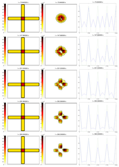
Figure 4.
Graph representing the evolution of the ECM (left), cell population (center), and the alignment functions (dotted) and (dashed) for the second example.
3.5. Third Example: Random ECM
The last scenario proposed a randomly-distributed matrix, which was modified to include a certain pathway. This resembled the case of tissue development, where the ECM directs the growing of the cell population, leading to complex structures.
For the cell distribution, we used the same initial conditions as in the first example (concentrated around with random velocities and small activity). Note that, in this case, measuring the alignment of the cells or the ECM with respect to a certain direction (or radial orientation), a priori, does not give any interesting information: the matrix originally did not have a preferred orientation. However, it is possible that, in subsequent steps, cells will remodel the ECM in a way that a preferential direction arises.
We expected that the cell population would concentrate in the established pathway, following this track, and few cells would remain outside the pathway. The behavior for the chemical L and the limiting activity was expected to be similar to the previous examples. Furthermore, we tracked and , to check possible remodeling on the ECM due to cell interactions or possible cell alignment caused by the creation of L and the remodeled matrix. Initial conditions and results are shown in Figure 5 and Figure 6, respectively.
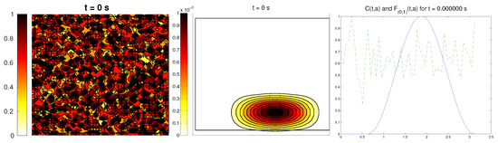
Figure 5.
Third example: initial conditions for the ECM fibers (oriented in the direction (0,1)), cell population, and the alignment functions (dotted) and (dashed).
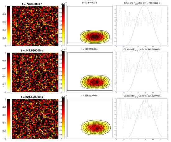
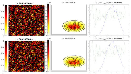
Figure 6.
Graph representing the evolution of the ECM (left), cell population (center), and the alignment functions (dotted) and (dashed) for the third example.
4. Conclusions
In the previous sections, we presented a multiscale approach to study cell movement, caused by two important driving phenomena, namely haptotaxis and chemotaxis. The modeling was performed at the microscopic scale, and the kinetic theory of active particles allowed us to obtain a mesoscopic model. Then, a hyperbolic scaling led to the macroscopic model.
The numerical experiments aimed to explore cell behavior through three selected case studies of biological significance, as proposed in [24]. The obtained results confirmed that cells tend to follow paths and to align according to the ECM structure. In this sense, it is worth noticing the analogy with crowd dynamics [33], vehicular traffic [34], or swarming phenomena [37], where individual entities also receive some stimulus from the surrounding environment, interact among themselves, and generate certain emergent behaviors.
The alignment functionals were introduced to measure numerically the alignment of the trajectories of the cells in order to compare with the structure of the surrounding ECM. These operators could be used in the future to establish and measure similar behaviors in more complex tissue structures, as they only need the density function of the given structure.
Finally, the macroscopic fluid model obtained from the KTAP theory includes an algebraic third equation binding the densities of the two main compounds of the ECM involved in the haptotaxis and chemotaxis processes with the macroscopic density of the cell-membrane receptors, which can be used to measure, at the level of these receptors, how far the kinetic model is from the macroscopic equilibrium counterpart.
Future research perspectives include some modifications of this model in order to consider more realistic ECM structures and/or other kinds of interactions within the cells and the extracellular matrix. For instance, the incorporation of the saturation dynamics of the medium due to cellular overpopulation [27] or the inclusion of two or more subpopulations of tumor cells interacting mutually and with the surrounding tissue [28]. Furthermore, a simple kinetic system could be proposed to include biological cancer mutations involving different cell populations (quiescent, active, etc.) with different abilities, in order to obtain a more realistic measure of the alignment and the invasion profile.
Author Contributions
D.N., J.N. and L.U. equally contributed to all phases of preparation of this article.
Funding
D.K. is partially funded by Consejo Nacional de Investigaciones Científicas y Técnicas Project PIP 11220150100500 CO, Agencia Nacional de Promoción Científica y Tecnológica Project PICT 2015-1066, and Secretaría de Ciencia y Técnica (UNC). J.N. is partially supported by Junta de Andalucía Project P12-FQM-954 and MINECO Project RTI2018-098850-B-I00.
Conflicts of Interest
The authors declare no conflict of interest.
References
- Ananthakrishnan, R.; Ehrlicher, A. The Forces Behind Cell Movement. Int. J. Biol. Sci. 2007, 3, 303–317. [Google Scholar] [CrossRef] [PubMed]
- Friedl, P.; Wolf, K. Tumour–cell invasion and migration: Diversity and escape mechanisms. Nat. Rev. Cancer 2003, 3, 362–374. [Google Scholar] [CrossRef] [PubMed]
- Wolf, K.; Friedl, P. Molecular mechanisms of cancer cell invasion and plasticity. Br. J. Dermatol. 2006, 154 (Suppl. 1), 11–15. [Google Scholar] [CrossRef] [PubMed]
- Keller, H.U.; Wissler, J.H.; Ploem, J. Chemotaxis is not a special case of haptotaxis. Experientia 1979, 35, 1669–1671. [Google Scholar] [CrossRef] [PubMed]
- Elosegui-Artola, A.; Bazellières, E.; Allen, M.D.; Andreu, I.; Oria, R.; Sunyer, R.; Gomm, J.J.; Marshall, J.F.; Jones, J.L.; Trepat, X.; et al. Rigidity sensing and adaptation through regulation of integrin types. Nat. Mater. 2014, 13, 631–637. [Google Scholar] [CrossRef] [PubMed]
- Wehrle–Haller, B. Assembly and disassembly of cell matrix adhesions. Curr. Opin. Cell Biol. 2012, 24, 569–581. [Google Scholar] [CrossRef]
- Guo, N.H.; Krutzsch, H.C.; Negre, E.; Zabrenetzky, V.S.; Roberts, D.D. Heparin-binding peptides from the Type I repeats of Thrombospondin. J. Biol. Chem. 1992, 267, 19349–19355. [Google Scholar]
- Guo, N.H.; Zabrenetzky, V.S.; Chandrasekaran, L.; Sipes, J.M.; Lawler, J.; Krutzsch, H.C.; Roberts, D.D. Differential roles of protein Kinase C and Pertussis Toxin–sensitive G-binding proteins in modulation of melanoma cell proliferation and motility by Thrombospondin 1. Cancer Res. 1998, 58, 3154–3162. [Google Scholar]
- Taraboletti, G.; Roberts, D.D.; Liotta, L.A. Thrombospondin–induced tumor cell migration: Haptotaxis and chemotaxis are meditated by different molecular domains. J. Cell Biol. 1987, 105, 2409–2415. [Google Scholar] [CrossRef]
- Berry, H.; Larreta-Garde, V. Oscillatory behavior of a simple kinetic model for proteolysisis during cell invasion. Biophys. J. 1999, 77, 655–665. [Google Scholar] [CrossRef]
- Erban, R.; Othmer, H. From signal transduction to spatial pattern formation in E. coli: A paradigm for multiscale modeling in biology. Multiscale Model. Simul. 2005, 3, 362–394. [Google Scholar] [CrossRef]
- Patlak, C. Random walk with persistence and external bias. Bull. Math. Biophys. 1953, 15, 311–338. [Google Scholar] [CrossRef]
- Keller, E.; Segel, L. Model for Chemotaxis. J. Theor. Biol. 1971, 30, 225–234. [Google Scholar] [CrossRef]
- Hillen, T.; Painter, K.J. A user’s guide to PDE models for chemotaxis. J. Math. Biol. 2009, 58, 183–217. [Google Scholar] [CrossRef] [PubMed]
- Chalub, F.A.; Markovich, P.; Perthame, B.; Schmeiser, C. Kinetic models for chemotaxis and their drift–diffusion limits. Monatsh. Math. 2004, 142, 123–141. [Google Scholar] [CrossRef]
- Othmer, H.G.; Hillen, T. The diffusion limit of transport equations II: Chemotaxis equations. SIAM J. Appl. Math. 2002, 62, 1222–1250. [Google Scholar] [CrossRef]
- Bellomo, N.; Bellouquid, A.; Nieto, J.; Soler, J. On the asymptotic theory from microscopic to macroscopic growing tissue models: An overview with perspectives. Math. Models Methods Appl. Sci. 2012, 22, 1130001. [Google Scholar] [CrossRef]
- Bellomo, N.; Bellouquid, A.; Tao, Y.; Winkler, M. Toward a mathematical theory of Keller-Segel models of pattern formation in biological tissues. Math. Models Methods Appl. Sci. 2015, 25, 1663–1763. [Google Scholar] [CrossRef]
- Arias, M.; Campos, J.; Soler, J. Cross-diffusion and traveling waves in porous-media flux-saturated Keller-Segel models. Math. Models Methods Appl. Sci. 2018, 28, 2103–2129. [Google Scholar] [CrossRef]
- Bellouquid, A.; Nieto, J.; Urrutia, L. About the kinetic description of fractional diffusion equations modeling chemotaxis. Math. Models Methods Appl. Sci. 2016, 26, 249–268. [Google Scholar] [CrossRef]
- Bellomo, N.; Bellouquid, A.; Chouhad, N. From a multiscale derivation of nonlinear cross-diffusion models to Keller-Segel models in a Navier-Stokes fluid. Math. Model. Methods Appl. Sci. 2016, 26, 2041–2069. [Google Scholar] [CrossRef]
- Oster, G.; Murray, J.D.; Harris, A.K. Mechanical aspects of mesenchymal morphogenesis. J. Embryol. Exp. Morphol. 1983, 78, 83–125. [Google Scholar]
- Mallet, D.G.; Pettet, G.J. A mathematical model of integrin–mediated haptotactic cell migration. Bull. Math. Biol. 2006, 68, 231–253. [Google Scholar] [CrossRef]
- Painter, K. Modelling cell migration strategies in the extracellular matrix. J. Math. Biol. 2009, 58, 511–543. [Google Scholar] [CrossRef]
- Chaplain, M.A.J.; Lolas, G. Mathematical modelling of cancer cell invasion of tissue: The role of the urokinase plasminogen activation system. Math. Models Methods Appl. Sci. 2005, 15, 1685–1734. [Google Scholar] [CrossRef]
- Kim, Y.; Jeon, H.; Othmer, H. The Role of the Tumor Microenvironment in Glioblastoma: A Mathematical Model. IEEE Trans. Biomed. Eng. 2017, 64, 519–527. [Google Scholar] [CrossRef]
- Zhigun, A.; Surulescu, C.; Uatay, A. Global existence for a degenerate haptotaxis model of cancer invasion. Z. Angew. Math. Phys. 2016, 67, 147. [Google Scholar] [CrossRef]
- Stinner, C.; Surulescu, C.; Uatay, A. Global existence for a go-or-grow multiscale model for tumor invasion with therapy. Math. Models Methods Appl. Sci. 2016, 11, 2163–2201. [Google Scholar] [CrossRef]
- Bellomo, N.; Knopoff, D.; Soler, J. On the difficult interplay between life, “complexity”, and mathematical sciences. Math. Models Methods Appl. Sci. 2013, 23, 1861–1913. [Google Scholar] [CrossRef]
- Bellouquid, A.; De Angelis, E.; Knopoff, D. From the modeling of the immune hallmarks of cancer to a black swan in biology. Math. Models Methods Appl. Sci. 2013, 23, 949–978. [Google Scholar] [CrossRef]
- Ajmone Marsan, G.; Bellomo, N.; Gibelli, L. Stochastic evolutionary differential games toward a systems theory of behavioral social dynamics. Math. Models Methods Appl. Sci. 2016, 26, 1051–1093. [Google Scholar] [CrossRef]
- Dolfin, M.; Knopoff, D.; Leonida, L.; Patti, D. Escaping the trap of “blocking”: A kinetic model linking economic development and political competition. Kinet. Relat. Models 2017, 10, 423–443. [Google Scholar] [CrossRef]
- Bellomo, N.; Bellouquid, A.; Knopoff, D. From the micro-scale to collective crowd dynamics. Multiscale Model. Simul. 2013, 11, 943–963. [Google Scholar] [CrossRef]
- Bellomo, N.; Bellouquid, A.; Nieto, J.; Soler, J. On the multiscale modeling of vehicular traffic: From kinetic to hydrodynamics. Discret. Cont. Dyn. Syst. Ser. B 2014, 19, 1869–1888. [Google Scholar] [CrossRef]
- Bellomo, N.; Gibelli, L. Toward a mathematical theory of behavioral-social dynamics for pedestrian crowds. Math. Mod. Methods Appl. Sci. 2015, 25, 2417–2437. [Google Scholar] [CrossRef]
- Bellomo, N.; Gibelli, L.; Outada, N. On the interplay between behavioral dynamics and social interactions in human crowds. Kinet. Relat. Model. 2019, 12, 397–409. [Google Scholar] [CrossRef]
- Bellomo, N.; Ha, S.-Y. A quest toward a mathematical theory of the dynamics of swarms. Math. Mod. Methods Appl. Sci. 2017, 27, 745–770. [Google Scholar] [CrossRef]
- Dimarco, G.; Pareschi, L. Numerical methods for kinetic equations. Acta Numer. 2014, 23, 369–520. [Google Scholar] [CrossRef]
- Outada, N.; Vauchelet, N.; Akrid, T.; Khaladi, M. From kinetic theory of multicellular systems to hyperbolic tissue equations: Asymptotic limits and computing. Math. Mod. Methods Appl. Sci. 2016, 26, 2709–2734. [Google Scholar] [CrossRef]
- Burini, D.; Chouhad, N. Hilbert method toward a multiscale analysis from kinetic to macroscopic models for active particles. Math. Mod. Methods Appl. Sci. 2017, 27, 1327–1353. [Google Scholar] [CrossRef]
- Banasiak, J.; Lachowicz, M. Methods of Small Parameter in Mathematical Biology; Series: Modeling and Simulation in Science, Engineering and Technology; Birkhäuser: Boston, MA, USA, 2014. [Google Scholar]
- Kelkel, J.; Surulescu, C. A multiscale approach to cell migration in tissue networks. Math. Mod. Methods Appl. Sci. 2012, 22, 1150017. [Google Scholar] [CrossRef]
- Nieto, J.; Urrutia, L. A multiscale modeling of cell mobility: From kinetic to hydrodynamics. J. Math. Anal. Appl. 2016, 433, 1055–1071. [Google Scholar] [CrossRef]
- Araujo, R.P.; McElwain, D.L.S. A history of the study of solid tumour growth: The contribution of mathematical modelling. Bull. Math. Biol. 2004, 66, 1039–1091. [Google Scholar] [CrossRef] [PubMed]
- Holden, H.; Karlsen, K.; Lie, K.; Risebro, N. Splitting Methods for Partial Differential Equations with Rough Solutions: Analysis and MATLAB Programs; EMS Series of Lectures in Mathematics; European Mathematical Society: Zürich, Switzerland, 2010. [Google Scholar]
- Changede, R.; Xu, X.; Margadant, F.; Sheetz, M.P. Nascent integrin adhesions form on all matrix rigidities after integrin activation. Dev. Cell 2015, 35, 614–621. [Google Scholar] [CrossRef]
- Welf, E.S.; Naik, U.P.; Ogunnaike, B.A. A spatial model for integrin clustering as a result of feedback between integrin activation and integrin binding. Biophys. J. 2012, 103, 1379–1389. [Google Scholar] [CrossRef][Green Version]
- Litvinov, B.A.; Mekler, A.; Shuman, H.; Bennett, J.S.; Barsegov, V.; Weisel, J.W. Resolving two-dimensional kinetics of the integrin αIIbβ3–fibrinogen interactions using binding-unbinding correlation spectroscopy. J. Biol. Chem. 2012, 287, 35275–35285. [Google Scholar] [CrossRef] [PubMed]
- Saragosti, J.; Calvez, V.; Bournaveas, N.; Perthame, B.; Buguin, A.; Silberzan, P. Directional persistence of chemotactic bacteria in a traveling concentration wave. Proc. Natl. Acad. Sci. USA 2011, 108, 16235–16240. [Google Scholar] [CrossRef]
© 2019 by the authors. Licensee MDPI, Basel, Switzerland. This article is an open access article distributed under the terms and conditions of the Creative Commons Attribution (CC BY) license (http://creativecommons.org/licenses/by/4.0/).