Article

An Improved Bat Algorithm Based on Lévy Flights and Adjustment Factors

1
Institute of Management Science and Engineering, and School of Business, Henan University, Kaifeng 475004, China
2
School of Business, Henan University, Kaifeng 475004, China
3
Institute of Intelligent Network Systems, and Software School, Henan University, Kaifeng 475004, China
4
Bristol Business School, University of the West of England, Bristol BS16 1QY, UK
*
Author to whom correspondence should be addressed.
Symmetry 2019, 11(7), 925; https://doi.org/10.3390/sym11070925
Submission received: 29 May 2019 / Revised: 29 June 2019 / Accepted: 13 July 2019 / Published: 15 July 2019

Abstract

:
This paper proposed an improved bat algorithm based on Lévy flights and adjustment factors (LAFBA). Dynamically decreasing inertia weight is added to the velocity update, which effectively balances the global and local search of the algorithm; the search strategy of Lévy flight is added to the position update, so that the algorithm maintains a good population diversity and the global search ability is improved; and the speed adjustment factor is added, which effectively improves the speed and accuracy of the algorithm. The proposed algorithm was then tested using 10 benchmark functions and 2 classical engineering design optimizations. The simulation results show that the LAFBA has stronger optimization performance and higher optimization efficiency than basic bat algorithm and other bio-inspired algorithms. Furthermore, the results of the real-world engineering problems demonstrate the superiority of LAFBA in solving challenging problems with constrained and unknown search spaces.

1. Introduction

Many problems in management can be treated as global optimization problems, and the need to efficiently solve large-scale optimization problems has prompted the development of bio-inspired intelligent optimization algorithms. For example, scholar Holland proposed a genetic algorithm (GA) based on the idea of evolution [1]; Kennedy and Eberhart proposed particle swarm optimization (PSO) [2,3] by referring to the swarm foraging behavior in nature; and Dorigo et al., inspired by ant foraging behavior, proposed the algorithm of ant colony optimization (ACO) [4]. In recent years, a variety of novel swarm intelligent optimization algorithms have been developed, such as bee colony algorithm [5], krill herd algorithm [6], cuckoo search algorithm [7,8] and moth flame optimization algorithm [9] etc. Although a meta-heuristic algorithm has the advantages of simple calculation steps and being easy to understand and implement, it also has the disadvantages of easily falling into local extreme value and low solution accuracy. Sergeyev et al. compared several widely used metaheuristic global optimization methods with Lipschitz deterministic methods by using operational zones, and simulation results show that, in some runs, the metaheuristic methods were getting stuck in the local solutions [10]. Therefore, it is of great significance to research and put forward swarm intelligence optimization algorithms with better performance to enrich the algorithm and expand the application field of the algorithm.
The bat algorithm (BA) is a metaheuristic optimization algorithm proposed by Yang [11]. The algorithm uses the bat’s echolocation capability to design an optimization strategy that iterates through frequency updates. The bat algorithm has the advantages of having less setting parameters, being easy to understand and implement, and having fast convergence. However, it also has drawbacks in balancing global and local search capabilities, it is easy to fall into a local optimum, and the solution accuracy is not high. To overcome these shortcomings, many scholars have made improvements to the bat algorithm. For instance, Ramli and other scholars, in order to improve the global search ability of the bat algorithm, put forward an enhanced bat algorithm (MBA) based on dimensional and inertia weight factor to enhance the convergence [12]. Banati and Chaudhary proposed a multimodal bat algorithm (MMBAIS) with improved search mechanism, which effectively alleviates the problem of early convergence and improves the convergence speed of the algorithm in later phase [13]. Al-Betar studied the alternative selection mechanism in the bat algorithm for global optimization [14]. Li added a mutation switch function to the standard bat algorithm and proposed a bat optimization algorithm (UGBA) that combines uniform variation and Gaussian variation [15]. Asma proposed a directional bat algorithm (dBA) to introduce directional echolocation in the standard bat algorithm to enhance the exploration and exploitation capabilities of the algorithm [16]. Al-Betar and Awadallah proposed an island bat algorithm (iBA) that uses the island model’s strategy for bat algorithms to enhance algorithm population diversity to avoid premature convergence [17].
In addition, many scholars are committed to expanding the application fields of bat algorithms. For example, Laudis and other scholars have proposed a multi objective bat algorithm (MOBA) to solve the problem in Very Large-Scale Integration (VLSI) design [18]. Tawhid and Dsouza proposed a hybrid binary bat enhanced particle swarm optimization algorithm (HBBEPSO) to solve the feature selection problems [19]. Osaba proposed an improved discrete bat algorithm (IBA) for solving symmetric and asymmetric traveling salesman problems [20]. Mohamed and Moftah proposed a novel multiobjective binary bat algorithm for simultaneous ranking and selection of keystroke dynamics features [21]. Hamidzadeh used the ergodicity of chaotic algorithm and the automatic conversion of bat algorithm global search and local search to construct a weighted SVDD method based on chaotic bat algorithm (WSVDD–CBA) for effective data description [22]. Qi and others proposed a discretized bat algorithm for solving vehicle routing problems with time windows [23]. Bekdaş and others used the bat algorithm to modify the tuning quality and proposed an effective method to solve the damper optimization problem [24]. Ameur and Sakly proposed a new hardware implementation of the bat algorithm’s field-programmable gate array (FPGA) [25]. Chaib and other scholars used the bat algorithm to optimize the design and adjust the novel fractional-order PID power system stabilizer [26]. Mohammad et al. used the bat algorithm to successfully solve the complex engineering problem of dam–reservoir operation [27]. In order to better solve the problem of mobile robot path planning, Liu et al. proposed a bat algorithm with reverse learning and tangent random exploration mechanism [28].
In order to improve the performance of the bat algorithm, this paper proposes an improved bat algorithm based on Lévy flights and adjustment factors (LAFBA). The search mechanism of Lévy flight is introduced to update the position of the bat algorithm, which can effectively help the algorithm maintain the diversity of the population and improve the global search ability. In addition, the introduction of the dynamic decreasing inertia weight and speed adjustment factor enables the algorithm to balance global exploration and local exploitation, improve the accuracy of the algorithm, and accelerate the later convergence speed.
The efficiency of the LAFBA is tested by solving 10 classical optimization functions and 2 structural optimization problems. The results obtained show that LAFBA is competitive in comparison with other state-of-the-art optimization methods.

2. Enhanced Bat Algorithm

2.1. Bat Algorithm

The bat algorithm is a swarm intelligent optimization algorithm that simulates the behavior of bats using the echolocation ability to prey. It realizes velocity and position update through the change of frequency f. The implementation of the algorithm is based on the following three idealized rules [11]:
Rule 1: Bats use echolocation to sense distance and can distinguish between prey and obstacles.
Rule 2: Bats fly randomly with the velocity v i at the position x i with a varying frequency f i (from a minimum frequency f m i n to a maximum frequency f m a x ) or a varying wavelength λ and sound loudness A 0 to search for prey. The wavelength (or frequency) of the emitted pulse can be automatically adjusted according to the proximity of the target, and the rate r of pulse emission, r [ 0 , 1 ] , is also adjusted.
Rule 3: Assume that the loudness varies from the largest positive value A 0 to the minimum constant value A m i n .
Based on the above rules, the position vector of the bat represents a solution in the search space. Since the global optimal position vector in the search space is not known a priori, the algorithm randomly initializes the bats. The initialize equation as follows:
x i , j = x l b + ( x u b x l b ) r a n d ,
for i t h bat, where i = 1 , 2 , , n ; j = 1 , 2 , , d ; n represents the population size, d represents the dimension of the search space. x l b and x u b are lower and upper bounds for j t h dimension, and r a n d is a random number between [0,1]. Bat individuals, in the d-dimensional search space, update frequency, velocity vector, and position vector according to the following equations:
f i = f m i n + ( f m a x f m i n ) β ,
v i t = v i t 1 + ( x i t x * ) f i ,
x i t = x i t 1 + v i t ,
where β is a random number between [0, 1]. x * represents the current global best solution, and the bat updates the velocity and position according to the change of frequency f.
When the bat performs a local search, the position update equation is as follows:
x n e w = x o l d + ε A t ,
where ε [ 1 , 1 ] which is set as 0.001 in this paper. A t represents the average loudness in current iteration.
As the bat approaches the prey, the loudness continues to decrease, while the rate of pulse emission increases. Loudness A i which is a vector of values for all bats, which assists in updating the bat location. Rate r i of pulse emission which is a vector for all bats controlling the diversification of bat algorithm. The update equation is as follows:
A i t = α · A i t 1 ,
r i t = r i 0 ( 1 e γ t ) .
Here, α is the pulse emission loudness attenuation coefficient. When t , for any value at α [ 0 , 1 ] and γ > 0 , it has A i t 0 and r i t r i 0 .

2.2. Dynamically Decreasing Inertia Weight
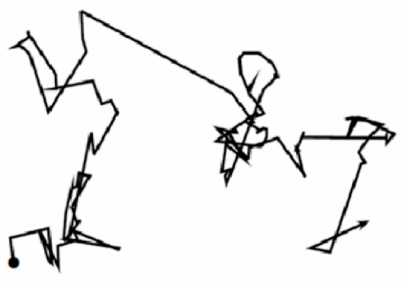
In the bat algorithm velocity update equation, right before the previous generation velocity v i t 1 is a constant term coefficient 1. The fixed coefficient is not conducive to the algorithm’s exploration of the global search space, and also reduces the flexibility of the bat individual in the algorithm, thus making it easy to fall into local optimum. The particle swarm optimization algorithm balances the global and local search by adjusting the inertia weight [29]. A larger inertia weight makes the individual’s change range larger, which is conducive to global exploration and local exploitation. A smaller inertia weight makes the individual change range smaller, which is advantageous for the algorithm to perform a local search on the optimization function. Inspired by this, this paper introduces the dynamic decreasing inertia weight, and changes the velocity update equation to
v i t = w i ( t ) v i t 1 + ( x i t x * ) f i ,
w i ( t ) = w m a x ( w m a x w m i n ) a r c t a n ( 4 t N _ g e n )
where w m a x and w m i n respectively represent the maximum and minimum weight, t represents the current number of iterations, and N _ g e n represents the maximum number of iterations. In this paper, w m a x takes a value of 0.9 and w m i n takes a value of 0.42. The inverse tangent function a r c t a n is a monotonically increasing function [30], so w i ( t ) is a monotonically decreasing function. The inertia of the early period is great, while the inertia of the late period is small, which can balance the global and local search of the algorithm well. In this paper, the arctangent function domain is [0,4]. The change of the arctangent function in the domain is gradually slowed down, making the decrease of w i ( t ) rapid in the early stage but slow in the late stage. The algorithm is converted from a fast global search to a slow local search, which can effectively improve the speed and accuracy of the algorithm.

2.3. Lévy Flights

In 1926, the French mathematician Paul Lévy proposed Lévy flights. Lévy flights phenomenon is very common in nature. The foraging activities of creatures, such as wasps, jackals, monkeys, and human hunting behaviors, are all consistent with the random motion model of Lévy’s flights [31]. For example, some herbivores randomly move around in a given area to find a source of grass, but if they cannot find it, they will quickly go to another area and then resume the previous way of walking. This can effectively avoid wasting time in a place with insufficient resource. Along the iterative process, an agglomeration phenomenon occurs in the individual bat algorithm, the population diversity is reduced, the global search ability is undermined, and the algorithm easily falls into premature convergence of local optimum. In order to solve this problem, this paper proposes to add the Lévy flight search mechanism to the bat algorithm, and modify the bat position vector update equation as below:
x i t = L é vy ( d ) x i t 1 + v i t .
Here, t is the current number of iterations, and d is the dimension of the search space. The Lévy flight is calculated as follows [32]:
L é vy ( x ) = 0.01 r 1 δ | r 2 | 1 ψ ,
where r 1 , r 2 are two random numbers in [0,1], ψ is a constant 1.5, and δ   is calculated as follows:
δ = ( Γ ( 1 + ψ ) sin ( π ψ 2 ) Γ ( 1 + ψ 2 ) ψ 2 ( ψ 1 2 ) ) 1 ψ ,
where Γ ( x + 1 ) = x   ! , 50 step sizes have been drawn to form a consecutive 50 steps of Lévy flights as shown in Figure 1 [32].
Figure 1 intuitively shows Lévy’s ability to suddenly move a long distance after several short distance movements. In this paper, the Lévy flight mechanism is introduced to the bat position update. On the one hand, it can effectively avoid the overreliance of the bat position change on the previous generation position information and ensure the diversity of the population. On the other hand, the random walk mode of Lévy flight that changes large steps suddenly after a series of small steps gives the bat individual the ability to jump suddenly, which helps the algorithm to jump out of the local optimum, avoid the premature convergence of the algorithm, and improve the global search ability.

2.4. Speed Adjustment Factor

In order to ensure the efficiency of the algorithm, this paper designs a speed adjustment factor c i ( t ) based on the dimension of the optimization function to be solved and the number of iterations of the algorithm, which is applied to the bat position update. Along the iteration progress, the speed adjustment factor changes from large to small, and the position movement step size changes from large to small, which satisfies the requirement of the algorithm for global search in the early iteration stage and local search in the later iteration stage, enabling the bat algorithm to search for the optimum when solving each generation of the movement in space. The position vector update equation in this article is as below:
x i t = L é vy ( d ) x i t 1 + v i t c i ( t )
c i ( t ) = θ d · e t N _ g e n .
Here, θ can be any value between [0,1], which is set as 0.01 in this paper. d represents the dimension of the search space. At the same dimensional level, c i ( t ) gradually decreases as the number of iterations increases, making the position update of the algorithm change from large-scale movement in the early stage to small-scale movement in the late stage, and accelerates the convergence speed of the algorithm. When the algorithm solves the function, the search difficulty will increase with the increase of dimension, and the problems of low solution accuracy and reduced solution speed may occur. With the increase of the solution dimension, the speed adjustment factor proposed in this paper will be maintained at a relatively low level, which can speed up the algorithm and improve the accuracy of the solution when solving high-dimensional functions.

2.5. The Pseudocode of the LAFBA

The dynamic declining inertia weight added in the velocity update can effectively balance the global and local search of the algorithm; the Lévy flight search mechanism introduced to the location update can ensure the diversity of the population and improve the global search ability of the algorithm, and the construction of the speed adjustment factor can effectively improve the solution accuracy and speed of the algorithm. The pseudocode of the LAFBA is shown as follows:
1. Define objective function f ( x ) , x = ( x 1 , , x d ) T
2. Set the initial value of population size n, α ,   γ , and N _ g e n
3. Initialize pulse rates r i and loudness A i
4. Initialize the bat population (Equation (1))
5. Evaluate and find x *   where   x * { 1 , 2 , , n }
6. while tN_gen
7.  for i = 1 to n
8.     Adjust frequency (Equation (2))
9.     Update inertia weight (Equation (9)) and L é vy ( d ) (Equation (11))
10.     Update the velocity (Equation (8)) and position vector (Equation (13)) of the bat
11.   if (rand > r i )
12.     Select a solution among the best solutions
13.     Generate a local solution around selected best (Equation (5))
14.   end if
15.     Evaluate objective function
16.   if (rand < A i & f( x i ) < f( x * ))
17.      x * = x i
18.     f( x * ) = f( x i )
19.     Increase r i (Equation (7))
20.     Reduce A i (Equation (6))
21.   end if
22.   if ( f ( x i t + 1 ) < f ( x * ) )
23.     Update the best solution x *
24.   end if
25.  end for
26. Rank the bats and find the current best x *
27.  t = t + 1
28. end while
29. Return x * , postprocess results and visualization

3. Numerical Simulation and Analysis

In order to test the performance of the improved algorithm proposed in this paper, ten standard optimization functions are selected [33], and the algorithm is compared with the standard bat algorithm (BA) [11], particle swarm optimization (PSO) algorithm [2], moth flame optimization (MFO) algorithm [9], sine cosine algorithm (SCA) [34], and butterfly optimization algorithm (BOA) [35].

3.1. Parameters Setting

We have tried to use different population sizes from n = 10 to 100, and we found that for most problems, n = 20 is sufficient. Therefore, we use a fixed population n = 20 for all simulations. In order to guarantee the comparability and fairness of the simulation experiment, the same parameters are set for the four algorithms: the population size n = 20, and the number of iterations N _ g e n = 500. For BA and LAFBA, α = γ = 0.9 , the sound loudness A i = 0.25 and the rate of pulse emission r i = 0.5. For PSO, we have used the standard version with learning parameters c1 = c2 = 2. For BOA, modular modality c is 0.01, power exponent a is increased from 0.1 to 0.3 and the probability switch p = 0.8.
The simulation environment is MATLAB 2014a, the operating system is Windows10 Home Chinese version, 4.00GB running memory, the processor is Intel(R) Core (TM) i5-6200U CPU @ 2.30 GHz 2.40GHz.

3.2. Standard Optimization Functions

Optimization functions are as below:
(1) Griewank Function
f 1 ( x ) = 1 4000 i = 1 d x i 2 i = 1 d cos ( x i i ) + 1
The function definition field is [−600, 600] and the theoretical optimal value is 0. This function is a continuous, differentiable, non-separable, scalable, multimodal multi-extreme function, with many local optima. The higher the function dimension, the more the number of local optima. It is extremely difficult to optimize and is thus often used to test the exploration and exploitation capabilities of the algorithm.
(2) Quartic Function
f 2 ( x ) = i = 1 d x i 4
The function definition field is [−1.28, 1.28], and the theoretical optimal value is 0. This function is a continuous, differentiable, separable, scalable, and high-dimensional unimodal function. Unimodal functions are often used to test the convergence speed of an algorithm.
(3) Ackley Function
f 3 ( x ) = 20 + e 20 e 0.2 1 d i = 1 d x i 2 e 1 d i = 1 d cos ( 2 π x i )
The function definition field is [−30, 30] and the theoretical optimal value is 0. This function is a continuous, differentiable, non-separable, scalable, and complex nonlinear multimodal function which is formed by the superposition of a moderately amplified cosine wave to an exponential function. The undulation of the function surface makes the search of this function more complicated, and there are a large number of local optima.
(4) Rastrigin Function
f 4 ( x ) = i = 1 d [ x i 2 10 cos ( 2 π x i ) + 10 ]
The function definition field is [−5.12, 5.12], and the function theory optimal value is 0. This function is a high-dimensional multimodal function. There are about 10d local minimum values in the solution space. The peak shape of the function fluctuates volatility, making the global search rather difficult.
(5) Schaffer Function
f 5 ( x ) = 0.5 + s i n 2 i = 1 d x i 2 0.5 [ 1 + 0.001 ( i = 1 d x i 2 ) ] 2
The function definition field is [−10, 10] and the theoretical optimal value is 0. The fluctuation is fierce, and it is difficult to find the global optimal value. The function graph presents a “four-corner hat” shape, which is a continuous, differentiable, non-separable, scalable, and typical multimodal function. The global optimal position is in the center of the brim, and the relative search area is very small.
(6) Sphere Function
f 6 ( x ) = i = 1 d x i 2
The function definition field is [−5.12, 5.12], and the theoretical optimal value is 0. This function is a continuous, differentiable, separable, scalable, and classic high-dimensional unimodal function.
(7) Axis Parallel Function
f 7 ( x ) = i = 1 d i x i 2
The function definition field is [−5.12, 5.12], and the theoretical optimal value is 0. This function is a unimodal function.
(8) Zakharov Function
f 8 ( x ) = i = 1 d x i 2 + ( 1 2 i = 1 d i x i ) 2 + ( 1 2 i = 1 d i x i ) 4
The function definition field is [−10,10], and the theoretical optimal value is 0. This function is a continuous, differentiable, non-separable, scalable, multimodal function.
(9) Schwefel 2.21 Function
f 9 ( x ) = m a x i { | x i | , 1 i d }
The function definition field is [−10, 10] and the theoretical optimal value is 0. This function is a continuous, non-differentiable, separable, scalable and unimodal function.
(10) Schwefel 1.2 Function
f 10 ( x ) = i = 1 d ( j = 1 i x j ) 2
The function definition field is [−5.12, 5.12], and the theoretical optimal value is 0. This function is a continuous, differentiable, non-separable, scalable, unimodal function.

3.3. Simulation Result Comparison and Analysis

The six algorithms are run on the above 10 optimization functions 30 times independently in dimensions 10, 30, and 100, and the function value obtained each time was recorded. According to the results of the algorithm in different dimensions, four criteria were collected and analyzed: best, worst, average, and standard deviation (SD). The data are shown in Table 1, Table 2 and Table 3.
With the statistical test, we can make sure that the results are not generated by chance [36]. The Wilcoxon rank-sum test [37,38] was conducted in this experiment and p_value < 0.05 and h = 1 indicate that the difference between the two data is significant. The statistical comparison results between LAFBA and other 5 algorithms are shown in Table 4.
With the increase of the solution dimension, the difficulty faced by the algorithm to achieve the best result increases, and the problems of low solution accuracy, slowing down of the solving speed, or even failure to achieve the best result may occur. Therefore, this paper sets the three dimensions of 10D, 30D, and 100D to observe the change in the performance of the six algorithms in different dimensions.
It should be noted that the best optimal solution obtained is highlighted in bold font. From the results presented in Table 1, Table 2 and Table 3, under different dimensions, LAFBA is able to obtain the best values among 10 test functions in comparison with the BA, PSO, MFO, and SCA. When d = 10, compared to the BOA, the LAFBA obtained better results on 9 benchmark functions except for F3. When d = 30/100, BOA obtained the better mean value of F9 was better than the LAFBA. As the dimension increases, the difficulty in solving the function increases. The improved LAFBA proposed in this paper can still solve each optimization function effectively with the smallest standard deviation, indicating a good stability of the function. That is, the robustness is good.
As shown in Table 4, both the p-value and h = 1 indicate the rejection of the null hypothesis of equal medians at the default 5% significance level. This means that the superiority of LAFBA is statistically significant. p _ value   0.05 and h = 0 have been underlined, and LAFBA is significantly different from BOA with the exception of F3.
In summary, the comparison with the other algorithms shows the superiority of LAFBA in several benchmarks. Among the six algorithms, LAFBA had the best performance.

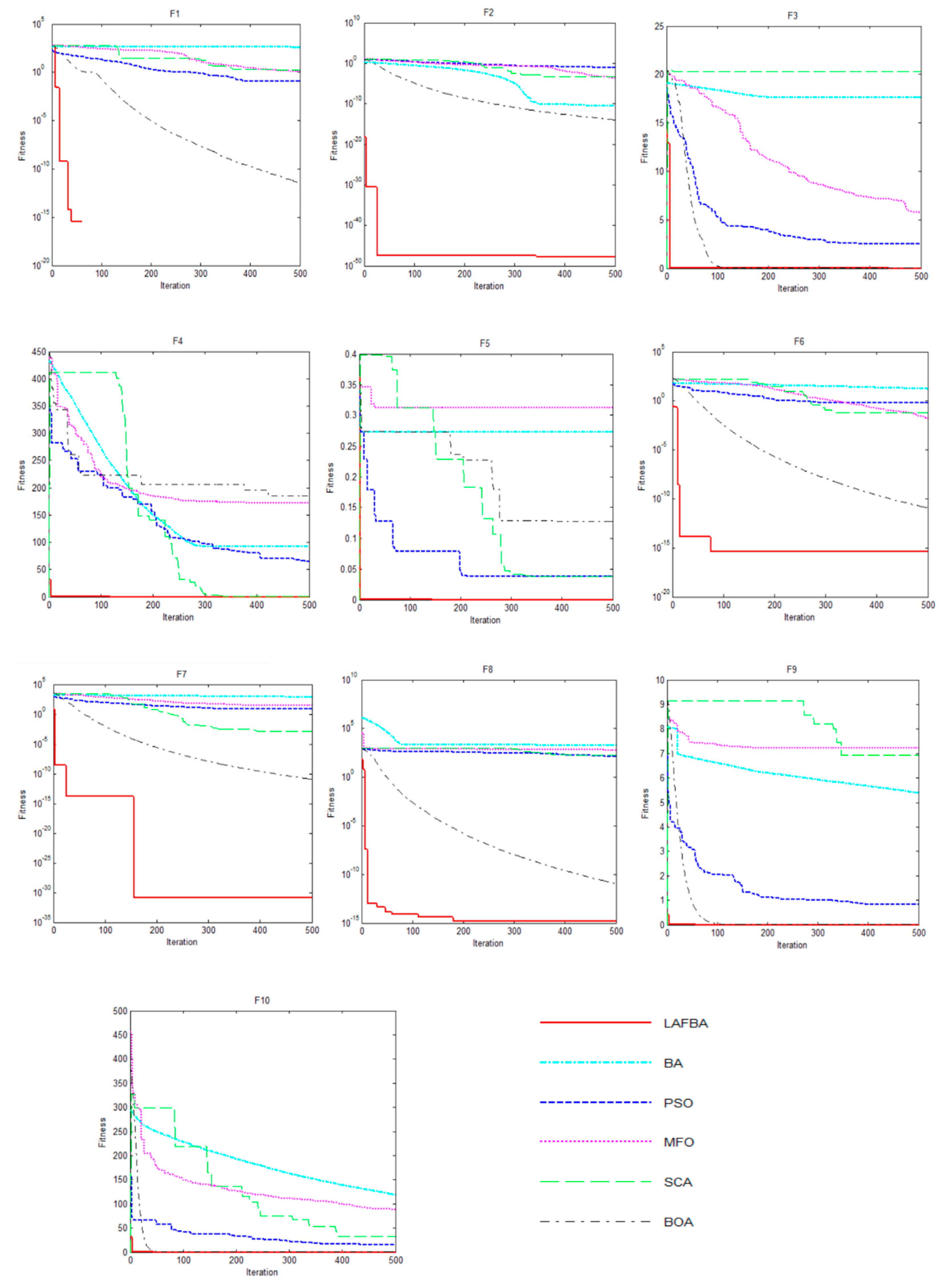
3.4. Convergence Curve Analysis

The convergence curve is an important indicator for the performance of the algorithm, through which we can see the convergence speed and the ability of the algorithm to jump out of the local optimum. For further illustration, the convergence curves of the LAFBA and other 5 algorithms with D = 30 on 10 benchmark functions are plotted in Figure 2.
The different trends of the six curves in Figure 2 show the difference in the performance of the six algorithms. Functions 2, 6, 7, 9, and 10 are unimodal functions, and are often used to compare the convergence speed and execution ability of the algorithm. Observing the contrast curve of the corresponding function convergence curve, the LAFBA proposed in this paper is effective in obtaining the optimal solutions with a faster convergence rate. The quality of the solution is much higher than BA, PSO, MFO, SCA, and BOA. Functions 1, 3, 4, 5, and 8 are multimodal functions, with a large number of local optima, which are extremely difficult to optimize. They are commonly used to test the global optimization ability of the algorithm. Observing the convergence curves of the corresponding functions, the inflection point in the curve shows that the LAFBA algorithm successfully jumps out of the local optimum and continues to optimize, while the other algorithms converge to the local optimum too early, resulting in a higher curve than the LAFBA. In summary, the LAFBA shows stronger optimization performance and higher optimization efficiency.

4. LAFBA for Classical Engineering Problems

This section further verifies the performance and efficiency of the LAFBA by solving two constrained real engineering design problems: tension/compression spring design, and welded beam design. These problems were widely discussed in the literature and have been solved to better clarify the effectiveness of the algorithms. In the LAFBA, the population size n = 20, and the number of iterations N_gen = 500.

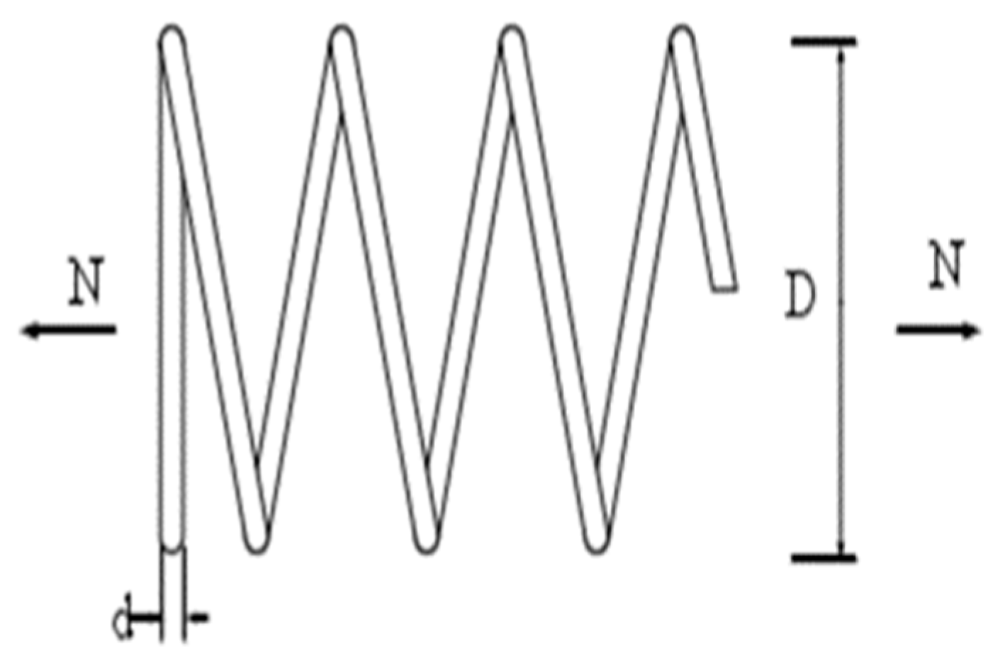
4.1. Tension/Compression Spring Design

The objective of this test problem is to minimize the weight of the tension/compression spring. Figure 3 shows the spring and its parameters [39,40]. The optimum design must satisfy constraints on shear stress, surge frequency, and deflection. This problem contains three constraint variables: the mean coil diameter (D), number of active coils (N), and wire diameter (d). The mathematical expression of tension/compression spring design problem is as follows:
Consider x = [ x 1   x 2   x 3 ] = [ d   D   N ] ,
Minimize f ( x ) = ( x 3 + 2 ) x 2 x 1 2 ,
Subject to g 1 ( x ) = 1 x 2 3 x 3 71785 x 1 4 0 ,
g 2 ( x ) = 4 x 2 2 x 1 x 2 12566 ( x 2 x 1 3 x 1 4 ) + 1 5108 x 1 2 1 0 ,
g 3 ( x ) = 1 140.45 x 1 x 2 2 x 3 0 ,
g 4 ( x ) = x 1 + x 2 1.5 1 0 ,
Variable range   0.05 x 1 2.00 , 0.25 x 2 1.30 , 2.00 x 3 15.0 .
There are several solutions for this problem found in the literature. This test case was solved using either mathematical techniques (constraints correction at constant cost [41] and penalty functions [40]) or meta-heuristics, such as GSA [42], PSO [43], evolution strategy (ES) [44], GA [45], and improved harmony search (HS) [46]. The best results of LAFBA are compared with 10 other optimization algorithms that were previously reported, as shown in Table 5.
From Table 5, compared with the GSA, PSO, ES, GA, and WOA, the LAFBA yielded better results for the tension/compression spring design problem. It can be seen that LAFBA outperforms all other algorithms except MFO, and the LAFBA algorithm is also the third-lowest-costing design.

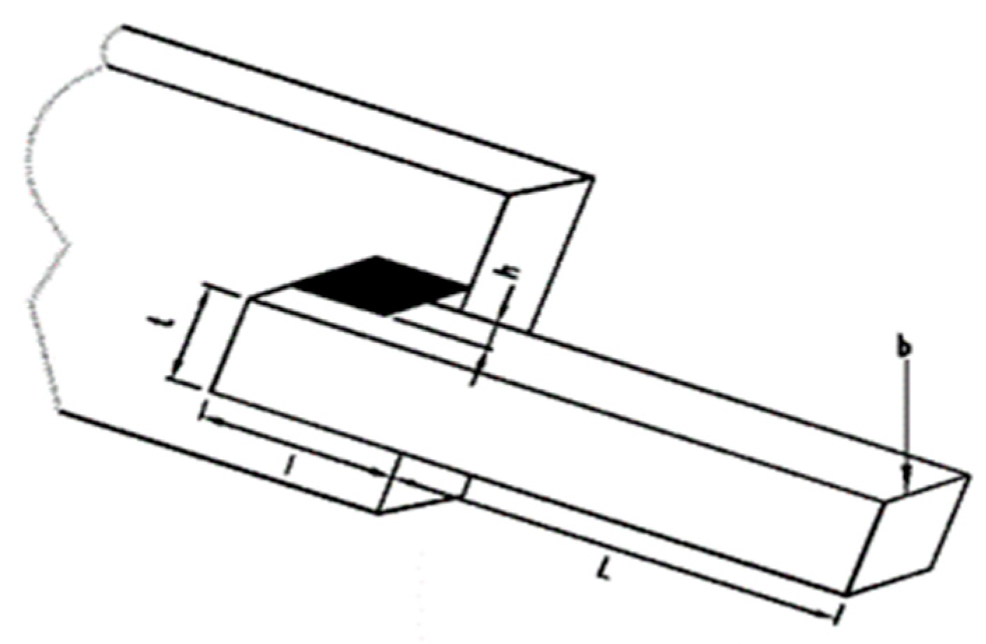
4.2. Welded Beam Design

The objective of this test problem is to minimize the fabrication costs of the welded beam design, and Figure 4 shows the welded beam and parameters involved in the design [45]. The optimum design must satisfy constraints on shear stress (τ) and bending stress in the beam (θ), buckling load ( P C ), and end deflection of the beam (δ). This problem contains four constraint variables: thickness of weld (h), length of the clamped bar (l), height of the bar (t), and thickness of the bar (b). The mathematical expression of welded beam design problem is as follows:
Consider x = [ x 1   x 2   x 3   x 4 ] = [ h   l   t   b ] ,
Minimize f ( x ) = 1.10471 x 1 2 x 2 + 0.04811 x 3 x 4 ( 14.0 + x 2 ) ,
Subject to g 1 ( x ) = τ ( x ) τ m a x 0 ,
g 2 ( x ) = σ ( x ) σ m a x 0 ,
g 3 ( x ) = δ ( x ) δ m a x 0 ,
g 4 ( x ) = x 1 x 4 0 ,
g 5 ( x ) = p p c ( x ) 0 ,
g 6 ( x ) = 0.125 x 1 0 ,
g 7 ( x ) = 0.10471 x 1 2 + 0.04811 x 3 x 4 ( 14.0 + x 2 ) 5.0 0 ,
Variable range   0.1 x 1 2 , 0.1 x 2 10 , 0.1 x 3 10 , 0.1 x 4 2 ,
where τ ( x ) = ( τ ) 2 + 2 τ τ x 2 2 R + ( τ ) 2 ,    τ = p 2 x 1 x 2 ,   τ = M R J ,
M = p ( L + x 2 2 ) ,    R = x 2 2 4 + ( x 1 + x 3 2 ) 2 ,
J = 2 { 2 x 1 x 2 [ x 2 2 12 + ( x 1 + x 3 2 ) 2 ] } ,    σ ( x ) = 6 P L x 4 x 3 2 ,   δ ( x ) = 4 P L 3 E x 3 3 x 4
P C ( x ) = 4.013 E x 3 2 x 4 6 36 L 2 ( 1 x 3 2 L E 4 G ) ,
p = 6000   lb ,   L = 14   in . , δ m a x = 0.25   in . ,
E = 30 × 106 psi, G = 12 × 106 psi,
τ m a x = 13 , 600   p s i , σ m a x = 30 , 000   p s i .
This problem was solved by GWO [49], GSA [42], Richardson’s random method, simplex method, Davidon–Fletcher–Powell, and Griffith and Stewart’s successive linear approximation [45]. The optimization results obtained by the proposed LAFBA for this problem were evaluated by comparing it with 15 other optimization algorithms that were previously reported, as shown in Table 6. Table 6 shows the best obtained results.
Table 6 shows that the LAFBA algorithm is able to find a similar optimal design compared to those of GWO, MVO, and CPSO. This shows that this algorithm is also able to provide very competitive results in solving this problem.

5. Conclusions

In this study, an improved bat algorithm based on Lévy flights and adjustment factors (LAFBA) is proposed. Three modifications have been embedded into the BA to increase its global and local search abilities and, consequently, have significantly enhanced the BA performance. In order to evaluate the effectiveness of the LAFBA, 10 benchmark functions and 2 real-world engineering problems are used. The results of the simulation experiment of 10 benchmark functions and Wilcoxon rank-sum test show that the proposed LAFBA was a great improvement in terms of exploration and exploitation abilities, solution accuracy, and convergence speed compared with the bat algorithm, and four other bio-inspired algorithms. In addition, the results of the LAFBA in solving classical engineering design problems were compared with several state-of-the-art algorithms and produced comparable results. As the LAFBA algorithm shows a stable performance, it can also be applied to other more challenging real-world optimization problems.

Author Contributions

Methodology, J.L.; Resources, X.R.; Writing—original draft, X.L.; Writing—review& editing, Y.L.

Acknowledgments

This study is supported by the National Natural Science Foundation of China (No. 71601071), the Science & Technology Program of Henan Province, China (No. 182102310886 and 162102110109), and an MOE Youth Foundation Project of Humanities and Social Sciences (No. 15YJC630079). We are particularly grateful to the suggestions of the editor and the anonymous reviewers which is greatly improved the quality of the paper.

Conflicts of Interest

The authors declare no conflict of interest.

References

  1. Holland, J.H. Erratum: Genetic Algorithms and the Optimal Allocation of Trials. Siam J. Comput. 1974, 3, 326. [Google Scholar] [CrossRef]
  2. Kennedy, J.; Eberhart, R. Particle swarm optimization. IEEE Int. Conf. Neural Netw. 1995, 2002, 1942–1948. [Google Scholar]
  3. Eberhart, R.; Kennedy, J. A new optimizer using particle swarm theory. In MHS’95. Proceedings of the Sixth International Symposium on Micro Machine and Human Science; IEEE Press: Piscataway, NJ, USA, 1995; pp. 39–43. [Google Scholar]
  4. Dorigo, M.; Colorni, V.A. Ant system: Optimization by a colony of cooperating agents. IEEE Trans. Syst. Man Cyber. Part B Cyber. 1996, 26, 29–41. [Google Scholar] [CrossRef] [PubMed]
  5. Karaboga, D. An Idea Based on Honey Bee Swarm for Numerical Optimization. TR-06; Erciyes University: Kayseri, Turkey, 2005. [Google Scholar]
  6. Gandomi, A.H.; Alavi, A.H. Krill herd: A new bio-inspired optimization algorithm. Commun. Nonlinear Sci. Numer. Simul. 2012, 17, 4831–4845. [Google Scholar] [CrossRef]
  7. Yang, X.S.; Deb, S. Cuckoo Search via Lévy flights. In Proceedings of the 2009 World Congress on Nature & Biologically Inspired Computing (NaBIC), Coimbatore, India, 9–11 December 2009; pp. 210–214. [Google Scholar]
  8. Yang, X.S.; Deb, S. Engineering Optimisation by Cuckoo Search. Int. J. Math. Modell. Numer. Optim. 2010, 1, 330–343. [Google Scholar] [CrossRef]
  9. Mirjalili, S. Moth-flame optimization algorithm: A novel nature-inspired heuristic paradigm. Knowl.-Based Syst. 2015, 89, 228–249. [Google Scholar] [CrossRef]
  10. Sergeyev, Y.D.; Kvasov, D.E.; Mukhametzhanov, M.S. Operational zones for comparing metaheuristic and deterministic one-dimensional global optimization algorithms. Math. Comput. Simul. 2017, 141, 96–109. [Google Scholar] [CrossRef]
  11. Yang, X.S. A New Metaheuristic Bat-Inspired Algorithm. Comput. Knowl. Technol. 2010, 284, 65–74. [Google Scholar]
  12. Ramli, M.R.; Abas, Z.A.; Desa, M.I.; Abidin, Z.Z.; Alazzam, M.B. Enhanced Convergence of Bat Algorithm Based on Dimensional and Inertia Weight Factor. J. King Saud Univ.-Comput. Inf. Sci. 2018. [Google Scholar] [CrossRef]
  13. Banati, H.; Chaudhary, R. Multi-Modal Bat Algorithm with Improved Search (MMBAIS). J. Comput. Sci. 2017, 23, 130–144. [Google Scholar] [CrossRef]
  14. Al-Betar, M.A.; Awadallah, M.A.; Faris, H.; Yang, X.S.; Khader, A.T.; Alomari, O.A. Bat-inspired Algorithms with Natural Selection mechanisms for Global optimization. Neurocomputing 2018, 273, 448–465. [Google Scholar] [CrossRef]
  15. Li, Y.; Pei, Y.H.; Liu, J.S. Bat optimization algorithm combining uniform variation and Gaussian variation. Control Decis. 2017, 32, 1775–1781. [Google Scholar]
  16. Chakri, A.; Khelif, R.; Benouaret, M.; Yang, X.S. New directional bat algorithm for continuous optimization problems. Expert Syst. Appl. 2017, 69, 159–175. [Google Scholar] [CrossRef] [Green Version]
  17. Al-Betar, M.A.; Awadallah, M.A. Island Bat Algorithm for Optimization. Expert Syst. Appl. 2018, 107, 126–145. [Google Scholar] [CrossRef]
  18. Laudis, L.L.; Shyam, S.; Jemila, C.; Suresh, V. MOBA: Multi Objective Bat Algorithm for Combinatorial Optimization in VLSI. Proc. Comput. Sci. 2018, 125, 840–846. [Google Scholar] [CrossRef]
  19. Tawhid, M.A.; Dsouza, K.B. Hybrid Binary Bat Enhanced Particle Swarm Optimization Algorithm for solving feature selection problems. Appl. Comput. Inf. 2018. [Google Scholar] [CrossRef]
  20. Osaba, E.; Yang, X.S.; Diaz, F.; Lopez-Garcia, P.; Carballedo, R. An improved discrete bat algorithm for symmetric and asymmetric Traveling Salesman Problems. Eng. Appl. Artif. Intell. 2016, 48, 59–71. [Google Scholar] [CrossRef]
  21. Mohamed, T.M.; Moftah, H.M. Simultaneous Ranking and Selection of Keystroke Dynamics Features Through A Novel Multi-Objective Binary Bat Algorithm. Future Comput. Inf. J. 2018, 3, 29–40. [Google Scholar] [CrossRef]
  22. Hamidzadeh, J.; Sadeghi, R.; Namaei, N. Weighted Support Vector Data Description based on Chaotic Bat Algorithm. Appl. Soft Comput. 2017, 60, 540–551. [Google Scholar] [CrossRef]
  23. Qi, Y.H.; Cai, Y.G.; Cai, H. Discrete Bat Algorithm for Vehicle Routing Problem with Time Window. Chin. J. Electron. 2018, 46, 672–679. [Google Scholar]
  24. Bekdaş, G.; Nigdeli, S.M.; Yang, X.S. A novel bat algorithm based optimum tuning of mass dampers for improving the seismic safety of structures. Eng. Struct. 2018, 159, 89–98. [Google Scholar] [CrossRef]
  25. Ameur, M.S.B.; Sakly, A. FPGA based hardware implementation of Bat Algorithm. Appl. Soft Comput. 2017, 58, 378–387. [Google Scholar] [CrossRef]
  26. Chaib, L.; Choucha, A.; Arif, S. Optimal design and tuning of novel fractional order PID power system stabilizer using a new metaheuristic Bat algorithm. Ain Shams Eng. J. 2017, 8, 113–125. [Google Scholar] [CrossRef] [Green Version]
  27. Mohammad, E.; Sayed-Farhad, M.; Hojat, K. Bat algorithm for dam–reservoir operation. Environ. Earth Sci. 2018, 77, 510. [Google Scholar]
  28. Liu, J.S.; Ji, H.Y.; Li, Y. Robot Path Planning Based on Improved Bat Algorithm and Cubic Spline Interpolation. Acta Autom. Sin. 2019. [Google Scholar]
  29. Shi, Y.; Eberhart, R. Modified particle swarm optimizer. Proc. IEEE ICEC Conf. Anchorage 1999, 69–73. [Google Scholar]
  30. Du, Y.H. Advanced Mathematics; Beijing Jiaotong University Press: Beijing, China, 2014. [Google Scholar]
  31. Ball, F.; Bao, Y.N. Predict Society; Contemporary China Publishing House: Beijing, China, 2007. [Google Scholar]
  32. Yang, X.S.; Karamanoglu, M.; He, X. Flower pollination algorithm: A novel approach for multiobjective optimization. Eng. Optim. 2014, 46, 1222–1237. [Google Scholar] [CrossRef]
  33. Jamil, M.; Yang, X.S. A Literature Survey of Benchmark Functions for Global Optimization Problems. Mathematics 2013, 4, 150–194. [Google Scholar]
  34. Mirjalili, S. SCA: A Sine Cosine Algorithm for solving optimization problems. Knowl.-Based Syst. 2016, 96, 120–133. [Google Scholar] [CrossRef]
  35. Arora, S.; Singh, S. Butterfly optimization algorithm: A novel approach for global optimization. Soft Comput. 2019, 23, 715–734. [Google Scholar] [CrossRef]
  36. Derrac, J.; García, S.; Molina, D.; Herrera, F. A practical tutorial on the use of nonparametric statistical tests as a methodology for comparing evolutionary and swarm intelligence algorithms. Swarm Evolut. Comput. 2011, 1, 3–18. [Google Scholar] [CrossRef]
  37. Wilcoxon, F. Individual Comparisons by Ranking Methods. Biom. Bull. 1945, 1, 80–83. [Google Scholar] [CrossRef]
  38. García, S.; Molina, D.; Lozano, M.; Herrera, F. A study on the use of non-parametric tests for analyzing the evolutionary algorithms’ behaviour: A case study on the CEC’2005 Special Session on Real Parameter Optimization. J. Heuristics 2009, 15, 617–644. [Google Scholar]
  39. Zhao, Z.Y. Introduction to optimum design. Probabilistic Eng. Mech. 1990, 5, 100. [Google Scholar]
  40. Belegundu, A.D.; Arora, J.S. A study of mathematical programming methods for structural optimization. Part I: Theory. Int. J. Numer. Methods Eng. 2010, 21, 1601–1623. [Google Scholar] [CrossRef]
  41. Kaveh, A.; Talatahari, S. An improved ant colony optimization for constrained engineering design problems. Eng. Comput. 2010, 27, 155–182. [Google Scholar] [CrossRef]
  42. Rashedi, E.; Nezamabadi-Pour, H.; Saryazdi, S. GSA: A Gravitational Search Algorithm. Inf. Sci. 2009, 179, 2232–2248. [Google Scholar] [CrossRef]
  43. He, Q.; Wang, L. An effective co-evolutionary particle swarm optimization for constrained engineering design problems. Eng. Appl. Artif. Intell. 2007, 20, 89–99. [Google Scholar] [CrossRef]
  44. Mezura-Montes, E.; Coello, C.A.C. An empirical study about the usefulness of evolution strategies to solve constrained optimization problems. Int. J. Gen. Syst. 2008, 37, 443–473. [Google Scholar]
  45. Coello Coello, C.A. Use of a Self-Adaptive Penalty Approach for Engineering Optimization Problems. Comput. Ind. 2000, 41, 113–127. [Google Scholar] [CrossRef]
  46. Mahdavi, M.; Fesanghary, M.; Damangir, E. An improved harmony search algorithm for solving optimization problems. Appl. Math. Comput. 2007, 188, 1567–1579. [Google Scholar] [CrossRef]
  47. Mirjalili, S.; Lewis, A. The Whale Optimization Algorithm. Adv. Eng. Softw. 2016, 95, 51–67. [Google Scholar] [CrossRef]
  48. Li, L.J.; Huang, Z.B.; Liu, F.; Wu, Q.H. A heuristic particle swarm optimizer for optimization of pin connected structures. Comput. Struct. 2007, 85, 340–349. [Google Scholar] [CrossRef]
  49. Mirjalili, S.; Mirjalili, S.M.; Lewis, A. Grey Wolf Optimizer. Adv. Eng. Softw. 2014, 69, 46–61. [Google Scholar] [CrossRef] [Green Version]
  50. Krohling, R.A.; Coelho, L.D.S. Coevolutionary Particle Swarm Optimization Using Gaussian Distribution for Solving Constrained Optimization Problems. IEEE Trans. Cyber. 2007, 36, 1407–1416. [Google Scholar] [CrossRef]
  51. Coello, C.; Carlos, A. constraint-handling using an evolutionary multi objective optimization technique. Civ. Eng. Environ. Syst. 2000, 17, 319–346. [Google Scholar] [CrossRef]
  52. Deb, K. Optimal design of a welded beam via genetic algorithms. AIAA J. 1991, 29, 2013–2015. [Google Scholar]
  53. Deb, K. An efficient constraint handling method for genetic algorithms. Comput. Methods Appl. Mech. Eng. 2000, 186, 311–338. [Google Scholar] [CrossRef]
  54. Lee, K.S.; Geem, Z.W. A new meta-heuristic algorithm for continuous engineering optimization: Harmony search theory and practice. Comput. Methods Appl. Mech. Eng. 2005, 194, 3902–3933. [Google Scholar] [CrossRef]
  55. MartÍ, V.; Robledo, L.M. Multi-Verse Optimizer: A nature-inspired algorithm for global optimization. Neural Comput. Appl. 2016, 27, 495–513. [Google Scholar]
  56. Askarzadeh, A. A novel metaheuristic method for solving constrained engineering optimization problems: Crow search algorithm. Comput. Struct. 2016, 169, 1–12. [Google Scholar] [CrossRef]
  57. Ragsdell, K.M.; Phillips, D.T. Optimal Design of a Class of Welded Structures Using Geometric Programming. J. Eng. Ind. 1976, 98, 1021–1025. [Google Scholar] [CrossRef]
Figure 1. A series of 50 consecutive steps of Lévy flights.
Symmetry 11 00925 g001
Figure 2. Convergence curve of F1–F10 function.
Symmetry 11 00925 g002
Figure 3. Tension/compression spring design problem.
Symmetry 11 00925 g003
Figure 4. Schematic view of welded beam design problem.
Symmetry 11 00925 g004
Table 1. Comparison results of Lévy flights and adjustment factors (LAFBA) and other five algorithms for benchmark functions with D = 10. BA, bat algorithm; PSO, particle swarm optimization; MFO, moth flame optimization; SCA, sine cosine algorithm; BOA, butterfly optimization algorithm.
AlgorithmFunctionBestWorstAverageSDFunctionBestWorstAverageSD
LAFBAF10000F607.89 × 10−161.05 × 10−161.98 × 10⁻¹⁶
BA1.27 × 1011.46 × 1027.99 × 1013.52 × 1017.48 × 10−28.76 × 1013.03 × 1012.63 × 101
PSO2.17 × 10−12.459.51 × 10−14.52 × 10−15.19 × 10−66.80 × 10−38.89 × 10−41.54 × 10⁻³
MFO7.92 × 10−117.58 × 10−11.51 × 10−11.44 × 10−19.89 × 10−171.48 × 10−131.10 × 10−142.82 × 10⁻¹⁴
SCA1.34 × 10−148.98 × 10−11.56 × 10−12.16 × 10−14.64 × 10−181.69 × 10−107.33 × 10−123.16 × 10⁻¹¹
BOA3.11 × 10−141.45 × 10−122.95 × 10−133.26 × 10−135.84 × 10−121.03 × 10−118.24 × 10−121.16 × 10⁻¹²
LAFBAF203.08 × 10−311.63 × 10−325.77 × 10⁻³²F701.53 × 10−151.67 × 10−163.98 × 10⁻¹⁶
BA6.74 × 10−147.29 × 10−132.85 × 10−131.51 × 10−134.63 × 10−64.76 × 1017.939.83
PSO2.62 × 10−118.69 × 10−77.48 × 10−81.91 × 10−75.19 × 10−66.80 × 10−38.89 × 10−41.54 × 10⁻³
MFO2.11 × 10−293.17 × 10−211.11 × 10−225.78 × 10−221.17 × 10−165.02 × 10−135.50 × 10−141.16 × 10⁻¹³
SCA1.15 × 10−307.54 × 10−203.46 × 10−211.42 × 10−209.03 × 10−184.87 × 10−123.70 × 10−139.31 × 10⁻¹³
BOA4.12 × 10−151.17 × 10−147.28 × 10−151.84 × 10−156.40 × 10−121.26 × 10−119.46 × 10−121.46 × 10⁻¹²
LAFBAF302.74 × 10−87.01 × 10−98.65 × 10−9F803.26 × 10−154.89 × 10−169.14 × 10⁻¹⁶
BA1.21 × 1011.94 × 1011.74 × 1011.511.318.01 × 1012.58 × 1011.92 × 101
PSO2.94 × 10−31.173.73 × 10−15.25 × 10−11.05 × 10−32.96 × 10−15.96 × 10−27.38 × 10⁻²
MFO2.99 × 10−85.094.07 × 10−11.052.45 × 10−62.51 × 1022.57 × 1015.80 × 101
SCA7.17 × 10−101.69 × 10−47.00 × 10−63.07 × 10−51.81 × 10−99.82 × 10−39.40 × 10−42.48 × 10⁻³
BOA1.65 × 10−96.14 × 10−93.49 × 10−91.20 × 10−97.47 × 10−121.14 × 10−119.61 × 10−121.09 × 10⁻¹²
LAFBAF409.59 × 10−141.50 × 10−142.48 × 10⁻¹⁴F901.23 × 10−82.51 × 10−94.09 × 10−9
BA1.79 × 1018.76 × 1014.78 × 1011.95 × 1011.655.083.469.33
PSO1.313.02 × 1019.416.932.14 × 10−22.94 × 10−18.88 × 10−25.66 × 10⁻²
MFO5.976.28 × 1012.70 × 1011.39 × 1019.20 × 10−24.801.371.16
SCA2.56 × 10−122.41 × 1012.446.641.09 × 10−73.34 × 10−33.59 × 10−46.97 × 10⁻⁴
BOA4.26 × 10−145.67 × 1013.10 × 1012.18 × 1013.77 × 10−95.34 × 10−94.50 × 10−94.30 × 10⁻¹⁰
LAFBAF506.11 × 10−168.23 × 10−171.52 × 10⁻¹⁶F1009.09 × 10−169.00 × 10−172.36 × 10⁻¹⁶
BA9.72 × 10−32.28 × 10−11.31 × 10−15.67 × 10−26.911.58 × 1026.14 × 1013.83 × 101
PSO9.72 × 10−37.82 × 10−22.67 × 10−21.68 × 10−27.82 × 10−49.71 × 10−22.89 × 10−23.03 × 10⁻²
MFO3.72 × 10−22.28 × 10−11.28 × 10−14.60 × 10−21.59 × 10−51.75 × 1013.356.25
SCA9.72 × 10−33.72 × 10−21.06 × 10−25.02 × 10−38.55 × 10−100.020479.25 × 10−40.003736
BOA3.72 × 10−28.08 × 10−27.18 × 10−21.47 × 10−25.97 × 10−121.11 × 10−119.02 × 10−121.38 × 10⁻¹²
Table 2. comparison results of LAFBA and other five algorithms for benchmark functions with D = 30.
AlgorithmFunctionBestWorstAverageSDFunctionBestWorstAverageSD
LAFBAF101.33 × 10−151.42 × 10−163.01 × 10⁻¹⁶F601.50 × 10−143.34 × 10−154.40 × 10⁻¹⁵
BA9.85 × 1015.36 × 1023.23 × 1021.08 × 1021.853.35 × 1021.86 × 1028.73 × 101
PSO5.80 × 10−23.46 × 10−11.66 × 10−17.21 × 10−21.49 × 10−19.03 × 10−13.74 × 10−11.56 × 10⁻¹
MFO9.48 × 10−12.71 × 1022.22 × 1016.11 × 1016.42 × 10−32.62 × 1013.559.05
SCA5.39 × 10−17.041.491.218.99 × 10−51.559.02 × 10−22.81 × 10⁻¹
BOA7.17 × 10−131.73 × 10−116.82 × 10−124.58 × 10−129.88 × 10−121.20 × 10−111.10 × 10−115.75 × 10⁻¹³
LAFBAF201.14 × 10−286.72 × 10−302.13 × 10⁻²⁹F701.75 × 10−133.06 × 10−145.03 × 10⁻¹⁴
BA2.18 × 10−116.16 × 10−82.18 × 10−91.14 × 10−84.00 × 1011.31 × 1035.37 × 1022.94 × 102
PSO4.78 × 10−42.691.16 × 10−14.96 × 10−12.223.37 × 1018.288.07
MFO3.59 × 10−62.86 × 10−32.43 × 10−45.34 × 10−43.87 × 10−27.87 × 1022.01 × 1022.24 × 102
SCA5.29 × 10−72.01 × 10−11.03 × 10−23.66 × 10−21.44 × 10−36.094.90 × 10−11.12
BOA8.92 × 10−151.56 × 10−141.15 × 10−141.35 × 10−151.10 × 10−111.37 × 10−111.23 × 10−117.91 × 10⁻¹³
LAFBAF301.04 × 10−72.42 × 10−83.32 × 10−8F803.70 × 10−147.39 × 10−151.15 × 10⁻¹⁴
BA1.36 × 1011.90 × 1011.75 × 1011.151.21 × 1012.27 × 1032.42 × 1024.05 × 102
PSO1.524.282.905.77 × 10−15.01 × 1014.20 × 1021.65 × 1028.14 × 101
MFO1.251.98 × 1011.51 × 1015.342.06 × 1029.81 × 1025.09 × 1021.97 × 102
SCA3.78 × 10−22.03 × 1017.698.974.31 × 1012.05 × 1021.26 × 1024.20 × 101
BOA5.53 × 10−97.04 × 10−96.24 × 10−93.84 × 10−108.71 × 10−121.18 × 10−111.05 × 10−117.86 × 10⁻¹³
LAFBAF402.49 × 10−122.57 × 10−136.51 × 10⁻¹³F906.42 × 10−81.62 × 10−82.38 × 10−8
BA5.97 × 1012.77 × 1021.43 × 1025.73 × 1013.808.416.171.05
PSO6.26E × 1011.39 × 1029.11 × 1012.09 × 1014.02 × 10−11.497.33 × 10−12.34 × 10⁻¹
MFO1.24 × 1022.84 × 1021.75 × 1023.39 × 1015.808.487.316.34 × 10−1
SCA1.4767452631.48 × 1024.68 × 1013.24 × 1011.116.683.981.26
BOA02.19 × 1023.93 × 1018.01 × 1014.30 × 10−95.59 × 10−95.13 × 10−92.75 × 10⁻¹⁰
LAFBAF501.64 × 10−142.62 × 10−154.82 × 10⁻¹⁵F1006.76 × 10−141.10 × 10−141.82 × 10⁻¹⁴
BA1.78 × 10−13.73 × 10−13.06 × 10−16.35 × 10−21.57 × 1022.68 × 1037.54 × 1024.79 × 102
PSO3.72 × 10−22.28 × 10−19.21 × 10−23.74 × 10−23.533.39 × 1011.32 × 1017.06
MFO3.12 × 10−13.73 × 10−13.42 × 10−11.72 × 10−27.391.65 × 1026.46 × 1013.86 × 101
SCA3.72 × 10−21.27 × 10−14.87 × 10−22.21 × 10−23.027.53 × 1013.54 × 1011.91 × 101
BOA7.85 × 10−21.27 × 10−11.17 × 10−11.87 × 10−29.36 × 10−121.23 × 10−111.11 × 10−116.22 × 10⁻¹⁴
Table 3. Comparison results of LAFBA and other five algorithms for benchmark functions with D = 100.
AlgorithmFunctionBestWorstAverageSDFunctionBestWorstAverageSD
LAFBAF101.67 × 10−152.87 × 10−165.31 × 10⁻¹⁶F601.81 × 10−135.31 × 10−146.00 × 10⁻¹⁴
BA5.33 × 1022.05 × 1031.31 × 1033.86 × 1024.33 × 1022.06 × 1031.15 × 1034.26 × 102
PSO1.111.03 × 1014.162.191.566.14 × 1011.35 × 1011.38 × 101
MFO4.57 × 1021.03 × 1036.68 × 1021.29 × 1021.27 × 1022.41 × 1021.90 × 1023.25 × 101
SCA1.40 × 1012.31 × 1021.01 × 1026.37 × 1013.029.46 × 1013.31 × 1012.13 × 101
BOA4.79 × 10−121.99 × 10−111.29 × 10−114.35 × 10−121.09 × 10−111.34 × 10−111.19 × 10−115.62 × 10⁻¹³
LAFBAF205.18 × 10−275.64 × 10−281.11 × 10⁻²⁷F705.14 × 10−121.14 × 10−121.90 × 10⁻¹²
BA1.58 × 10−71.512.02 × 10−14.22 × 10−12.37 × 1032.11 × 1049.63 × 1034.51 × 103
PSO1.281.31 × 1014.692.882.12 × 1024.43 × 1036.72 × 1029.23 × 102
MFO2.761.33 × 1017.312.535.75 × 1031.40 × 1049.27 × 1032.35 × 103
SCA1.619.524.291.892.39 × 1023.80 × 1031.17 × 1037.31 × 102
BOA1.10 × 10−141.58 × 10−141.29 × 10−141.02 × 10−151.19 × 10−111.53 × 10−111.35 × 10−118.61 × 10⁻¹³
LAFBAF301.53 × 10−73.86 × 10−85.92 × 10−8F801.57 × 10−121.68 × 10−133.74 × 10⁻¹³
BA1.51 × 1011.92 × 1011.78 × 1018.52 × 10−13.44 × 1021.74 × 1038.28 × 1022.86 × 102
PSO4.568.126.129.17 × 10−17.99 × 1023.06 × 1031.52 × 1035.23 × 102
MFO1.93 × 1011.99 × 1011.97 × 1011.62 × 10−12.39 × 1035.00 × 1033.99 × 1036.68 × 102
SCA8.282.06 × 1011.68 × 1014.749.96 × 1022.00 × 1031.44 × 1032.26 × 102
BOA5.14 × 10−96.81 × 10−95.85 × 10−93.48 × 10−108.18 × 10−121.19 × 10−111.04 × 10−118.34 × 10⁻¹³
LAFBAF403.41 × 10−111.03 × 10−111.11 × 10⁻¹¹F901.80 × 10−74.13 × 10−86.89 × 10−8
BA2.02 × 1028.14 × 1024.60 × 1021.49 × 1025.369.197.041.06
PSO4.28 × 1027.24 × 1025.65 × 1026.46 × 1011.192.841.774.13 × 10−1
MFO8.15E × 1021.10 × 1039.19 × 1027.34 × 10−38.959.699.372.02 × 10−1
SCA3.24 × 1016.68 × 1022.59 × 1021.43 × 1028.509.479.152.18 × 10−1
BOA03.51 × 10−11.17 × 10−26.40 × 10−24.66 × 10−95.89 × 10−95.28 × 10−92.71 × 10−10
LAFBAF502.66 × 10−135.69 × 10−147.18 × 10⁻¹⁴F1001.96 × 10−125.81 × 10−137.43 × 10⁻¹³
BA3.73 × 10−14.72 × 10−14.44 × 10−12.52 × 10−22.47 × 1031.37 × 1046.31 × 1032.72 × 103
PSO7.82 × 10−23.12 × 10−11.92 × 10−15.56 × 10−21.29 × 1024.26 × 1022.55 × 1027.16 × 101
MFO4.60 × 10−14.76 × 10−14.70 × 10−13.45 × 10−34.13 × 1029.28 × 1026.59 × 1021.39 × 102
SCA1.78 × 10−13.47 × 10−12.83 × 10−14.28 × 10−24.48 × 1021.38 × 1037.26 × 1021.94 × 102
BOA1.27 × 10−11.54 × 10−11.30 × 10−15.35 × 10−39.76 × 10−121.43 × 10−111.21 × 10−111.06 × 10⁻¹²
Table 4. Results of Wilcoxon rank-sum test for LAFBA and other algorithms on 10 test functions with D = 30.
FLAFBA vs. BALAFBA vs. PSOLAFBA vs. MFOLAFBA vs. SCALAFBA vs. BOA
p_Valuehp_Valuehp_Valuehp_Valuehp_Valueh
F19.78 × 10−1219.78 × 10−1219.78 × 10−1219.78 × 10−1219.78 × 10−121
F26.51 × 10−1116.50 × 10−1116.51 × 10−1116.51 × 10−1116.48 × 10−111
F33.71 × 10−1113.71 × 10−1113.71 × 10−1113.71 × 10−1110.1116550
F41.24 × 10−1111.24 × 10−1111.24 × 10−1111.24 × 10−1111.14 × 10−061
F52.23 × 10−1111.68 × 10−1119.12 × 10−1212.52 × 10−1112.55 × 10−111
F66.51 × 10−1116.51 × 10−1116.51 × 10−1116.51 × 10−1116.45 × 10−111
F76.51 × 10−1116.51 × 10−1116.51 × 10−1116.51 × 10−1116.46 × 10−111
F86.50 × 10−1116.50 × 10−1116.50 × 10−1116.50 × 10−1116.46 × 10−111
F96.51 × 10−1116.51 × 10−1116.51 × 10−1116.51 × 10−1110.0432011
F106.50 × 10−1116.51 × 10−1116.51 × 10−1116.51 × 10−1116.46 × 10−111
Table 5. Comparison results for tension/compression spring design problem.
AlgorithmsOptimal Values for VariablesOptimal Cost
dDN
GSA [42]0.0502760.32368013.5254100.0127022
PSO (Ha and Wang) [43]0.0517280.35764411.2445430.0126747
ES (Coello and Montes) [44]0.0519890.36396510.8905220.0126810
GA(Coello) [45]0.0514800.35166111.6322010.0127048
Improved HS (Mmahdavi et al.) [46]0.0511540.34987112.0764320.0126706
MFO [9]0.0519940.36410910.8684220.0126669
WOA [47]0.0512070.34521512.0040320.0126763
Montes and Coello [48]0.0516430.35536011.3979260.0126980
Constraint correction (Arora) [41] 0.0500000.31590014.2500000.0128334
Mathematical optimization (Belegundu) [40]0.0533960.3991809.18540000.0127303
LAFBA0.0516630.35607411.3334000.0126720
Table 6. Comparison results for welded beam design problem.
AlgorithmsOptimal Values for VariablesOptimal Cost
hltb
GWO [49]0.2056763.4783779.036810.2057781.72624
GSA [42]0.1821293.85697910.00000.2023761.87995
CPSO [50]0.2023693.5442149.0482100.2057231.72802
GA(Coello) [51]N/AN/AN/AN/A1.8245
GA(Deb) [52]N/AN/AN/AN/A2.3800
GA(Deb) [53] 0.24896.17308.17890.25332.4331
HS (Lee and Geem) [54]0.24426.23318.29150.24432.3807
MVO [55]0.20543.473199.0445020.205691.72645
GSA [56]0.20573.47049.03660.20571.7248
MFO [9]0.20573.47039.03640.20571.72452
WOA [47]0.2053963.4842939.0374260.2062761.730499
Random [57]0.45754.73135.08530.66004.1185
Simplex [57]0.27925.62567.75120.27962.5307
David [57]0.24346.25528.29150.24442.3841
Approx [57]0.24446.21898.29150.24442.3815
LAFBA0.1847061853.6426556919.1348973580.2052540531.7287

