Article

Segmentation of Articular Cartilage and Early Osteoarthritis based on the Fuzzy Soft Thresholding Approach Driven by Modified Evolutionary ABC Optimization and Local Statistical Aggregation

Department of Cybernetic and Biomedical Engineering, VŠB—Technical University of Ostrava, 17, listopadu 15, 708 33 Ostrava–Poruba, Czech Republic
*
Author to whom correspondence should be addressed.
Symmetry 2019, 11(7), 861; https://doi.org/10.3390/sym11070861
Submission received: 22 May 2019 / Revised: 20 June 2019 / Accepted: 25 June 2019 / Published: 2 July 2019

Abstract

:
Articular cartilage assessment, with the aim of the cartilage loss identification, is a crucial task for the clinical practice of orthopedics. Conventional software (SW) instruments allow for just a visualization of the knee structure, without post processing, offering objective cartilage modeling. In this paper, we propose the multiregional segmentation method, having ambitions to bring a mathematical model reflecting the physiological cartilage morphological structure and spots, corresponding with the early cartilage loss, which is poorly recognizable by the naked eye from magnetic resonance imaging (MRI). The proposed segmentation model is composed from two pixel’s classification parts. Firstly, the image histogram is decomposed by using a sequence of the triangular fuzzy membership functions, when their localization is driven by the modified artificial bee colony (ABC) optimization algorithm, utilizing a random sequence of considered solutions based on the real cartilage features. In the second part of the segmentation model, the original pixel’s membership in a respective segmentation class may be modified by using the local statistical aggregation, taking into account the spatial relationships regarding adjacent pixels. By this way, the image noise and artefacts, which are commonly presented in the MR images, may be identified and eliminated. This fact makes the model robust and sensitive with regards to distorting signals. We analyzed the proposed model on the 2D spatial MR image records. We show different MR clinical cases for the articular cartilage segmentation, with identification of the cartilage loss. In the final part of the analysis, we compared our model performance against the selected conventional methods in application on the MR image records being corrupted by additive image noise.

1. Introduction

The articular cartilage is focused on a resistance to the compressive forces, load distribution, and with a combination of the synovial fluid, frictionless movement of the articular joint components. Structurally, the articular cartilage contains approximately 70–80% of fluid and 20–30% of cellular matrix of the chondrocytes, having a sparse distribution. The chondrocytes are responsible for homeostatic and repair processes, modulating composition of the fluid-like macromolecular network [1,2].
From the view of the clinical practice, osteoarthritis (OA) represents one of the most prevalent musculoskeletal disorders, causing a substantial part of the elderly population. Furthermore, there is an unfavorable prediction of the next increase in the future time due to the population aging [1,2,3]. A severe complication, which relate to OA are structural changes of the articular cartilage, causing its degradation, having progressive and irreversible consequences. Also, it is closely linked with adjacent joint structures pathologies, including, for instance, the subchondral bone and meniscus [4,5,6].
In the clinical diagnosis of the OA, the structural diagnosis is essential. This assessment is based on the indication of a definite osteophyte in anterior-posterior X-ray images. Such image modalities are capable of finding the joint space, but they are not sensitive to a progression of the cartilage loss. This method is frequently used for indication of the effectiveness of disease-modifying OA drugs [7,8,9,10]. Another imaging alternative for the articular cartilage is the ultrasound. [11] As well as the radiographs, ultrasound imaging is not capable of reliably imaging the articular cartilage morphological structure. Thus, tiny structural changes cannot be properly investigated [12,13].
In comparison with others, magnetic resonance imaging (MRI) enables a structural visualization of all the tissues related with the OA disease, including the articular cartilage. A great benefit of MRI is qualitative and quantitative morphologic assessment [14,15]. MRI-based approaches enable characterization and quantification of the articular cartilage biochemical composition. Such techniques include the relaxometry measurements, including T2, T1, T2* imaging and T1rho mapping, sodium imaging, delayed gadolinium-enhanced MRI of cartilage (dGEMRIC), glycosaminoglycan specific chemical exchange saturation transfer (gagCEST), and diffusion weighted imaging (DWI). Compositional MR-based imaging techniques have a strong potential to serve as a quantitative, reproducible, and non-invasive techniques for OA investigation [16,17,18]. On the other hand, current needs of articular cartilage clinical imaging are focused on autonomous extraction and modeling of the cartilage structure, with the regard of the OA. Such segmentation techniques should be capable of extracting the physiological structure of the articular cartilage, and classify the pathological tissues affected by OA. A summary drawback of the MR imaging is a relative smaller proportion of the articular cartilage, regarding the whole knee area. Therefore, the early pathological cartilage loss is insufficiently differentiated from the healthy cartilage, as it is shown in the Figure 1.
In this paper, we are focused on the regional segmentation of the knee MR images. Particularly, we are focusing on extraction and modeling of the physiological structure of the articular cartilage, with regard of identification of the early cartilage loss caused by OA. We propose a multiregional segmentation scheme, which is based on soft fuzzy thresholding, where forming the individual segmentation classes is driven by the modified evolutionary artificial bee colony (ABC) optimization scheme. This hybrid segmentation method, including fuzzy based thresholding and evolutionary computing, offers promising results of the cartilage segmentation even in a noisy environment. We provide testing and evaluation of the proposed segmentation method, applied on the native clinical MR knee images, containing OA, as well as the synthetically degraded MR images by deterministic noise generators to evaluate robustness of the proposed method.
The organization of the paper is as follows. In Section 2 we describe the recent methods for the cartilage segmentation, which are grouped based on the level of a user’s interaction. Section 3 deals with the proposal of the segmentation model for the cartilage segmentation. We define the basic concept of the soft thresholding, including intensity segmentation and spatial aggregation. Further, we introduce the optimization procedure of the soft thresholding based on the modified ABC algorithm. Section 4 brings the results of the proposed model for the cartilage segmentation. We are especially focused on the healthy cartilage segmentation and indication of the early cartilage loss, caused by the early osteoarthritis. Section 5 deals with the quantitative comparison and objective evaluation of the proposed method against selected state of the art segmentation techniques. Section 6 brings the discussion about the results of the proposed segmentation scheme for the cartilage segmentation.

2. Recent Methods of Cartilage Segmentation

This chapter describes recent segmentation models for the cartilage segmentation. Generally, there are various reasons for the cartilage segmentation, as it is modeling of the morphological cartilage structure, or the pathological finding objective assessment. On the one hand, the ideal segmentation method should work as autonomous as possible, on the other hand, different MR sequences provide cartilage imaging with different intensity manifestation. Therefore, a development of the fully autonomous system allowing for precise segmentation is still the topic of the recent development. Individual methods are grouped by level from the user’s interaction [19,20].
The manual segmentation, performed by the clinical experts, has been perceived as a gold standard for the segmentation method’s performance assessment. It is a substantially demanding and time-consuming approach which may represent analysis over several hours depending on the image size, quality, and particular pathological findings. Furthermore, this methods lack of relevant reproducibility is caused by subjective error and requires special training [21,22].
From a practical point of view, a balance between the algorithm’s performance, preciseness, robustness, and the user interaction level should be kept. An ideal automatic segmentation algorithm would restrict the user’s interaction to a minimum and, at the same time, maximize the algorithm’s preciseness. There are several factors making this task complicated. The articular cartilage thickness is thin, less than a millimeter. Also, a significant issue is having sufficient contrast achieved between the cartilage and adjacent tissues. Furthermore, the cartilage tissue is not homogenous in certain parts. Therefore, the automatic algorithm should be trained in order to recognize these patterns. The fully cartilage segmentation includes the following techniques: Texture analysis [22], supervised learning [23], statistical methods (active shape models and adaptive template matching) [21], graph-cut methods [22,24], and edge detection methods [19,20,25,26].
The semi-automatic segmentation methods are aimed to reduce the user’s interaction as much as possible. These methods commonly require the initialization, meaning that the user is required to specify certain parameters driving the segmentation process. The semi-automatic methods may be divided as follows: Intensity-based [27], thresholding, watershed [28], edge detection [29], energy minimization [30], Live Wire [31], and active contours [30,32].

3. Materials and Methods

In the comparison with the adjacent knee tissues, the articular cartilage manifestation belongs to a different part of the intensity range. By this assumption, it can be modelled by the regional segmentation identifying individual tissues by their intensity spectrum. Since different MR devices and sequences produce the knee images with various resolutions and image quality, there is not a unified finite intensity range reliably approximating the cartilage area. Furthermore, we must consider that the presence of the image noise and the MR artifacts will significantly modify the intensity distribution, which can never be excluded from the MR image records. The proposed segmentation method compensates these facts by the way that creates adjustable image regions on the base of the pixel’s intensity and spatial information driven by evolutionary optimization with the cartilage image features. The overall flow chart of the proposed method is depicted in Figure 2.
In the proposed method, we tried to avoid using the image preprocessing operations to not modify native clinical information. We only use a selection of region of the interest (RoI) in order to expand the area of the articular cartilage due to its small size when comparing with the other knee structures like bones. Unlike many methods for the cartilage segmentation proposed in the recent literature dealing with the cartilage extraction, the proposed method is focused on the cartilage surface analysis, which enables the mapping of tiny structural changes, representing the early cartilage loss.
The basic version of the soft thresholding in [33] utilizes a decomposition of the image area based on the fuzzy sets with clustering and consequent statistical aggregation. This approach represents a general regional image segmentation procedure, not regarding any particular tissues. We bring an optimization of the soft thresholding based on evolutionary computing, selecting the best configuration of the fuzzy class distribution. It is a hybrid segmentation scheme, utilizing the soft thresholding approach which is driven by the evolutionary optimization. Furthermore, in the proposed approach, the configuration of the fuzzy sets are not only done by the clustering, but the real cartilage features are incorporated. This improves accuracy and robustness of the proposed segmentation model.

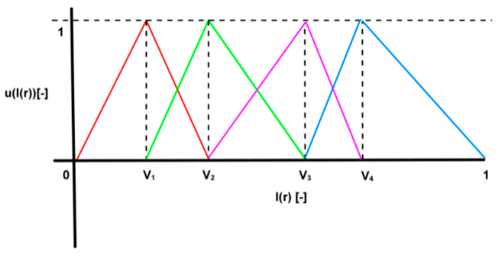
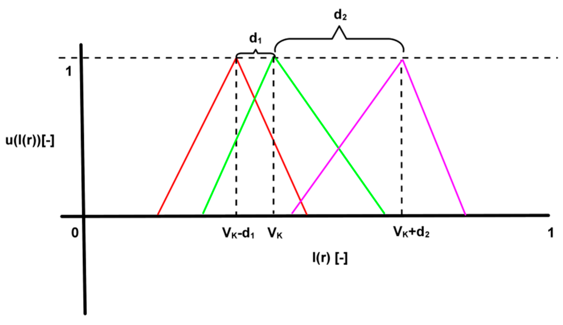
3.1. Soft Segmentation of Intensity Spectrum

A soft multiregional segmentation supposes that the knee image area may be decomposed into a predefined number of the segmentation classes, which should correspond with individual tissues, having different intensity spectrum. In order to perform this task, the MR image histogram is approximated by a sequence of the triangular fuzzy membership functions. In this configuration, the image histogram values are approximated by the fuzzy membership values, so that each pixel will have a certain membership in each segmentation class. We process the image data, represented by 256 gray levels, so the fuzzy approximation is done by: ( 0 ; 255 ) ( 0 ; 1 ) . Membership values ( 0 ; 1 ) assign a level of the membership for each pixel from the range ( 0 ; 255 ) of gray levels. In this scheme, membership 0 stands for a pixel that does not belong to this class, contrarily membership 1 indicates the full-assignment to this class. In this scheme, the original pixel’s distribution expressed by the image histogram is replaced by the system of membership functions (Figure 3).
For construction of such a segmentation model, the triangular functions are defined. Individual triangular membership functions are defined based on its centroid. In this case, a centroid is represented by the triangular membership vertex. Supposing we have a system of p triangular membership classes: μ n ( x ) , n = 1 ,   2 ,   ,   p , we need to determine an equivalent system of centroids represented by the triangular feature vector: V = { V 1 ,   V 2 , ,   V p } , where V represents a vertex of a respective triangular function. An illustration of a system of the triangular functions approximating the MR image histogram is depicted in Figure 3.
A membership of pixel k in the image I(k), in the nth segmentation class is given as μ n ( k ) . When using the triangular function, a membership satisfies a condition:
n = 1 p μ n ( I ( k ) ) = 1
Thus, each pixel is transformed into a space of the fuzzy membership, defined as follows:
μ ( I ( k ) ) = [ μ 1 ( I ( k ) )   μ 2 ( I ( k ) )   μ p ( I ( k ) ) ]
When using the triangular fuzzy membership functions, only two adjacent elements of μ ( I ( k ) ) are non-zero. A system of the triangular membership functions satisfies the following requirements:
  • Complete division: k ,   μ l ( k ) ,   1 l p , so that μ l ( k ) > 0 .
  • Consistency: if μ n ( k 0 ) = 1 , then μ m ( k 0 ) = 0 ,   n m .
  • Normality: max ( μ n ( k ) ) = 1 .
  • Intersection between adjacent fuzzy sets: μ n ( k 0 ) = μ n + 1 ( k 0 ) = 0.5   | |   μ n 1 ( k 0 ) = μ n ( k 0 ) = 0.5 .

3.2. Process of Centroids Extraction

The original idea of the centroid extraction deals with the clustering methods. Nevertheless, the clustering methods require a choice of the initial centroid selection. When selecting improper initial centroids, it may result to inaccurate segmentation results, which badly reflect the knee structures. Note that there is not a versatile method for the initial cluster’s selection.
In the proposed method, we use a hybrid scheme for the centroid’s definition, based on the K-means clustering and modified ABC evolutionary optimization algorithm. From the K-means, we only use the found centroids, consequently serving for the initial forming of the triangular fuzzy functions, not representing the articular cartilage. The physiological cartilage centroid, as well as others, are found by a modified version of the ABC algorithm utilizing the physiological cartilage features.

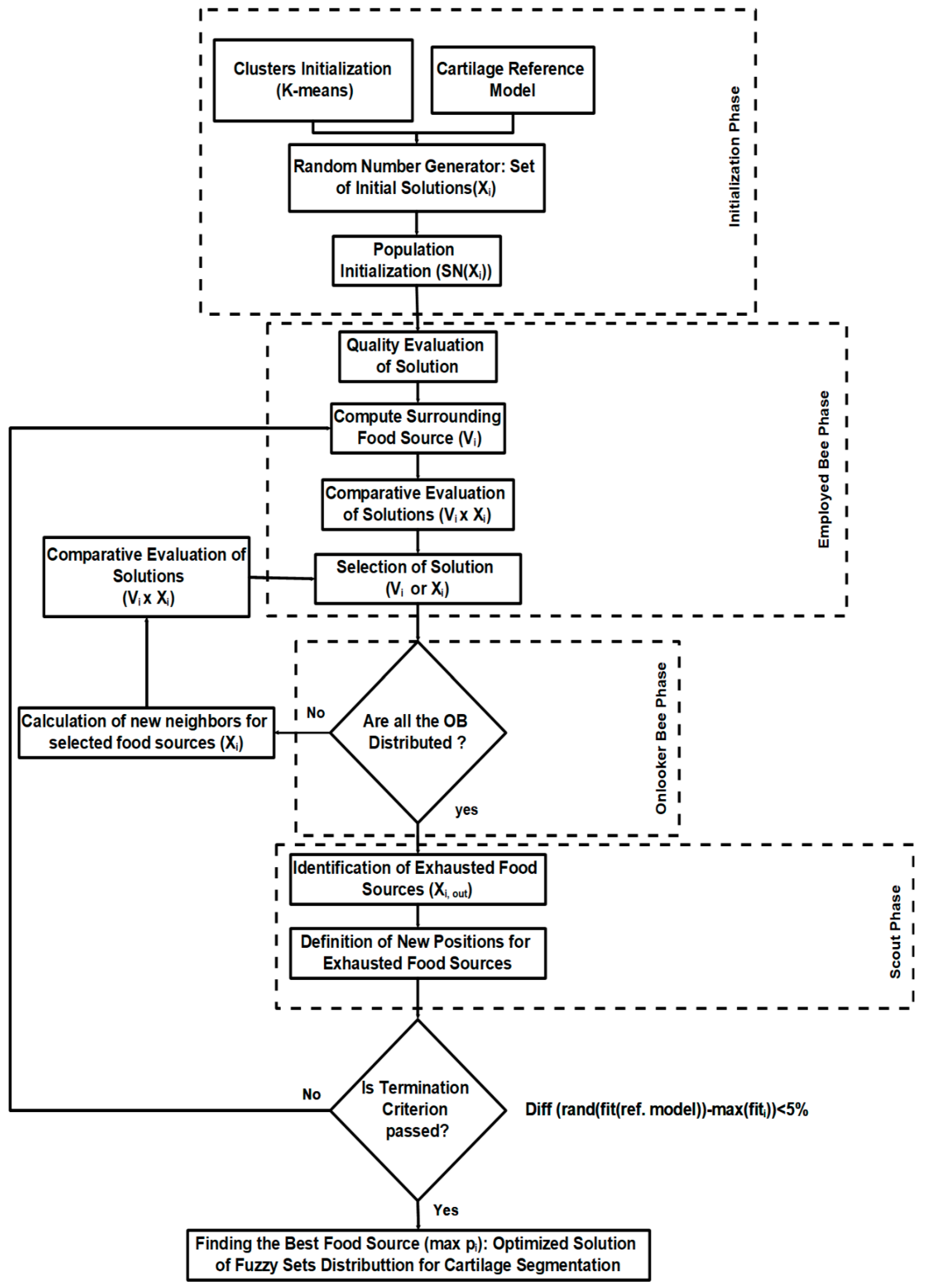
3.3. Modified ABC Algorithm

ABC algorithm represents an evolutionary optimization algorithm inspired by a bee swarm seeking for the food [34,35,36,37]. In this algorithm, there are three groups of artificial bees: Employed bees (EB), onlooker bees (OB), and scout bees (SB). Each kind of the bees search for food sources. A food source represents one solution of the optimization problem. Each such solution particularly represents one configuration of the fuzzy class’s distribution for the image segmentation. A proper distribution of the fuzzy classes is a crucial step in the whole segmentation algorithm. Within the optimization procedure, we are searching for the configuration of the fuzzy sets having the maximal compactness. Therefore, we use the entropy for an evaluation of each fuzzy sets configuration. In our approach, we use the Kapur’s entropy as an evaluator of each configuration. In this context, we suppose that a higher entropy corresponds with better fuzzy sets distribution. The optimization problem is determined by finding the optimal distribution of fuzzy classes centroids based on the fitness function. The fitness function is based on the Kapur’s entropy calculation for each region. The optimization process searches for maximization of the entropy function of the segmentation model. For this task we use the fitness function as an evaluator of individual solutions.
Firstly, we suppose an equal number of EB and OB. We also suppose that one EB has one food source. The parameter X i = { X i , 1 ,   X i , 2 ,   , X i , p } represents ith solution in the bee swarm, where p stands for a size of the dimension, and in other words these are the number of optimized centroids of the multiregional soft segmentation model.
In this point, we specify X i solution in the bee’s swarm. In the conventional ABC algorithm, these solutions are given randomly. In the proposed method, we utilize the real cartilage features in a combination with the random number generator. In order to determine representative cartilage features, we use the estimator of the physiological cartilage intensity average value. In order to perform this task, we employed the segmentation model based on the active contours driven by minimization of the Gaussian energy [32]. This model can adopt the healthy cartilage structure. Since the healthy cartilage is represented by the nearly focused intensity spectrum, not containing intensity fluctuations, it may be well approximated by the Gaussian distribution. Figure 4 shows an example of the physiological cartilage modeling by using the active contour driven by Gaussian energy minimization.
We analyzed the sample of the MR knee images containing 260 image records. 200 of these images were used for investigation of the healthy cartilage features, the rest of them were used for testing of the proposed model with the target of the osteoarthritis identification. All the images were acquired in MR 1.5T with the fat suppression technique, within the period 2014–2017. Images have the unified spatial resolution 1200 × 800 px and dynamical range ( 0 ; 255 ) gray levels. All the images were acquired in the DICOM format. For each of them we obtained the binary model reflecting the physiological structure of the cartilage. Based on these models, we compute an estimation of the intensity spectrum based on two alternative methods for interval estimation.
Firstly, we selected the median interval estimation with the reliability 95%. Estimation of median range for the physiological cartilage is given:
x ^ 0.5 1.57 ( x ^ 0.75 x ^ 0.25 ) n ; x ^ 0.5 + 1.57 ( x ^ 0.75 x ^ 0.25 ) n
where xp represents 100 p% quantile and n represents the range of sample data (we analyzed 200 MR image records).
The second alternative, for the physiological cartilage average value estimation, is the Gastwirth median. The Gastwirth median is calculated based on the selected median by the following expression:
x ^ G S T = 0.4 . x ^ 0.5 + 0.3 . ( x ^ 0.33 + x ^ 0.66 )
Estimation of the Gastwirth median is given:
x ^ G S T 1.57 x ^ 0.75 x ^ 0.25 n ; x ^ G S T + 1.57 x ^ 0.75 x ^ 0.25 n
We computed the following parameters for median estimation:
x ^ 0.25 = 204.39 x ^ 0.5 = 210.96 x ^ 0.75 = 215.33
The median interval estimation (Equation (3)) is calculated:
210.96 1.57 ( 215.33 204.33 ) 150 ; 210.96 + 1.57 ( 215.33 204.33 ) 150 209.54 ; 212.37
The parameters for calculation of the Gastwirth median are follows:
x ^ 0.5 = 210.96 x ^ 0.33 = 207.043 x ^ 0.66 = 213.49 x ^ G S T = 210.54
Then, the Gastwirth median is calculated:
210.54 1.57 215.33 204.33 150 ; 210.54 + 1.57 215.33 204.33 150 209.12 ; 211.95
Based on the selected interval estimations, we computed a median estimation for the physiological cartilage from 200 MR images (Table 1). Results from both of the methods do not exhibit significant statistical differences. For the ABC algorithm, we use an intersection of both intervals reported in Table 1. Note that we worked with the MR images represented by 256 shade levels.
Based on the results from Table 1, we determine estimation of the physiological cartilage as follows: I c = 209 ; 211 . Firstly, we define a scheme for the X i in the Equation (6).
X i = R i , L C L
where R i , L 0 ; 1 stands for the random numbers of ith solution and L denotes a vector of segmentation classes: L = { 1 ,   2 , , p } . Vector C L stands for the ith sequence of the centroids generated by the K-means clustering in the form: C L = { C 1 ,   C 2 , C p   } . In each C L , we have to identify and replace centroid representing the cartilage area. In order to do this task, we use the following formulation:   C i , c a r t i l a g e = min k L | C i ,   k I c R i | . C c a r t i l a g e replaces a respective centroid from C L for each solution in the swarm based on the minimal distance where I c R i stands for randomly chosen value from Ic.
When X i is generated, each OB generates a new candidate solution V i in the X i neighborhood. V i is given as following:
V i k = X i k + ϕ i k × ( X i k X j k )
where X j k represents a random candidate solution ( i j ), k represents a random index, given: k { 1 ,   2 ,   p } and function ϕ i k represents a generator of the random numbers in the range: [ 0.1 ; 0.1 ] . Based on the selection, the X i and V i are compared on the base of their fitness functions. If fitVi > fitXi, Vi is stored in the memory. Otherwise, a new V i is generated. The maximal number of such repetitions is controlled by the choice limit L v (we use: L v =10). When the L v is exhausted, the X i is perceived as an exhausted food source.
In the second stage of the ABC, OB test and evaluate the individual solutions from a global view. This process is done based on the probabilistic selection (Equation (8)), performed as many times, as many solutions we have for X i .
P i = f i t i j = 1 S N f i t j
It is supposed that more optimal solution has a greater P i . When the X i is selected, the V i is determined from Equation (7) and their fitness functions are compared. As same as in the first stage, a solution having greater fitness function is selected.
The last part of the algorithm are the scouts, seeking for the new food sources, instead of exhausted food sources. When flagging an exhausted food source as X i , e , consequently scout finds a new one, and the whole procedure is repeated within a predefined number of iterations (NI) (we use NI = 200). A new food source is given by the expression:
X i k = l b j + r a n d ( 0 , 0.1 ) × ( u b j l b j )
where l b ,   u b represent lower and upper limit of dimension, respectively. In the proposed segmentation method these limits represent boarders of the normalized intensity spectrum (0;1). In the final step, a solution having the biggest P i is selected as the most optimal solution for the centroids specification.

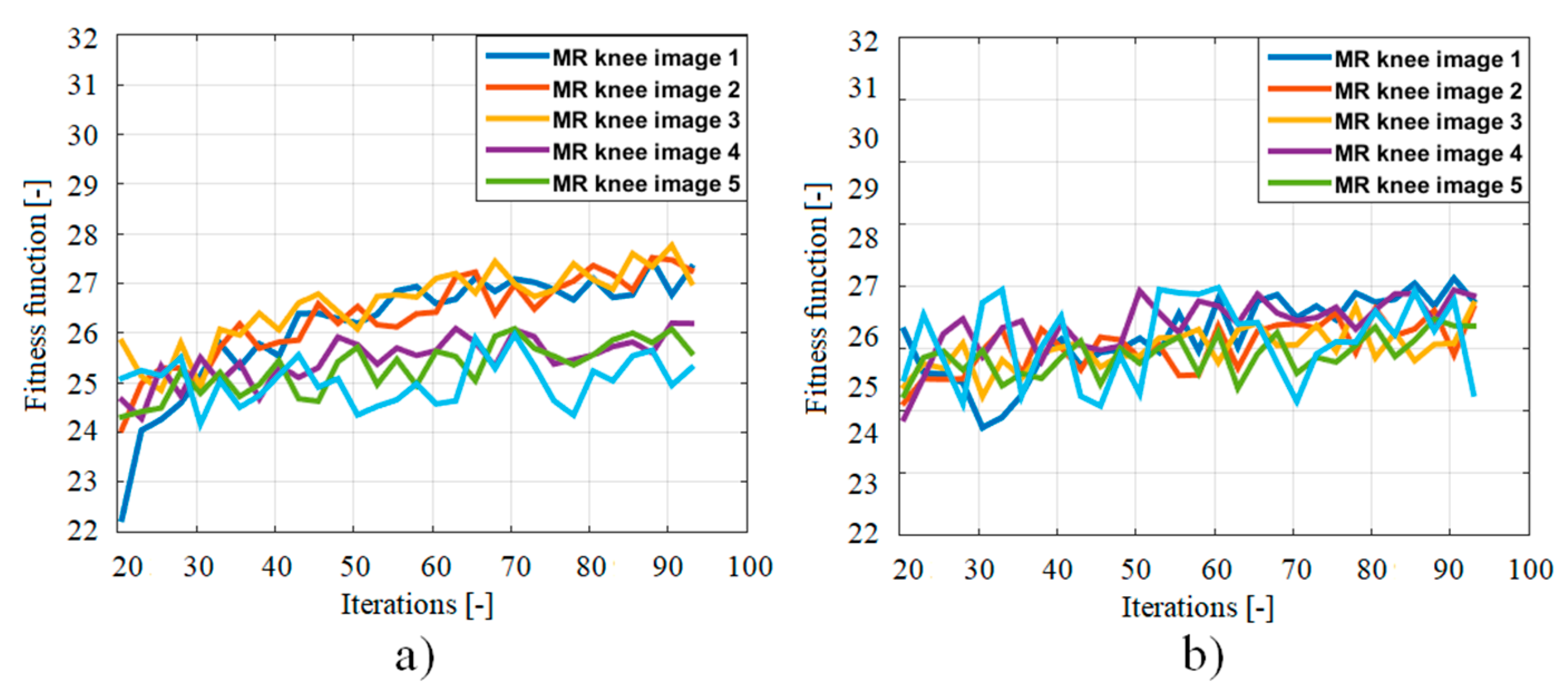
3.4. Features Extraction Based on Fitness Function

Generally, it is supposed that for each segmentation class theoretically unlimited alternatives may be defined, better or worse reflect features of a respective knee structure. Each alternative should be considered based on the histogram features. This situation (for V k segmentation class) is illustrated on the Figure 5. The key aspect of the entire genetic optimization is a fitness function, which globally evaluate a respective segmentation class in order to determine an optimal placement of the segmentation classes to reliably approximate individual knee tissues.
An important aspect is an optimization criterion defining a fitness function. Theoretically, a finite set of features characterizing the articular cartilage intensity manifestation may be used. We suppose that the articular cartilage represents a homogenous compact structure on the MR imaging. When intensity fluctuations are presented, they indicate pathological findings. Based on these facts, Kapur’s entropy is used for the fitness function design. It is supposed that the higher entropy respective fuzzy function has the more optimal solution represents. Regarding manifestation of the articular cartilage on the MR images, the MR signal of the physiological cartilage is represented by concentrated and compact intensity values, without significant intensity fluctuations. This fact is also proved by the interval estimations reported in Table 1. In such configurations, it can be supposed that a region of the cartilage, containing the intensity values with a high probability will be approximated with a higher entropy. In this optimization procedure, we search for the maximization of the Kapur’s entropy of the segmentation model. The higher entropy we obtain for the particular X i , the more suitable solution is. Firstly, the probability p k of each gray level h ( k ) is represented by the relative frequency divided by a total number of gray levels, defined as follows:
p k = h ( k ) k = 0 L 1 h ( k )
We suppose that the MR image contains L intensity components, where: k = 0, 1, 2, …, L − 1. Each segmentation class represented by the triangular function is described by two thresholds t and centroid V in the form: { t i , 1 , V i ,   t i , 2 } where i stands for order of the segmentation class. The Thresholding vector T of the segmentation model, containing p classes is given:
T = [ { t 1 , 1 , V 1 ,   t 1 , 2 } ,   { t 2 , 1 , V 2 ,   t 2 , 2 } , , { t p , 1 , V p ,   t p , 2 } ]
The Kapur’s entropy enables measuring compactness and separability of the segmentation classes is defined by the following equations:
H 1 = i = t 1 , 1 t 1 , 2 p i ω 1 ln ( p i ω 1 ) , ω 1 = i = t 1 , 1 t 1 , 2 p i
H 2 = i = t 2 , 1 t 2 , 2 p i ω 2 ln ( p i ω 2 ) , ω 2 = i = t 2 , 1 t 2 , 2 p i
H p 1 = i = t p 1 , 1 t p 1 , 2 p i ω p 1 ln ( p i ω p 1 ) , ω p 1 = i = t p 1 , 1 t p 1 , 2 p i
H p = i = t p , 1 t p , 2 p i ω p ln ( p i ω p ) , ω p = i = t p , 1 t p , 2 p i
By this way, the multiregional thresholding is configured as a multi-dimensional optimization problem. Based on the maximization, the fitness function, assessing each solution, is defined with the target of the entropy maximization (Equation (16)).
f i t i = arg m a x ( k = 1 p s H k )
In Figure 6, we present a structure of the ABC evolutionary optimization for the cartilage segmentation. In order to track an evolution of the fitness function on the NI, we report the convergence characteristics for the fitness function (Figure 7). In this regard, an important parameter, influencing the fitness function is a number of the food sources X i .
The following Table 2 brings the statistical evaluation of the ABC optimization for six segmentation classes. The testing was done for 60 MR knee images containing OA. We present extract of six images. In the testing, we evaluated the best, worst, median, and standard deviation of the fitness function (Equation (16)).
Another challenging issue of the segmentation procedure is the time complexity of the segmentation. In this regard, we evaluated the time complexity for different image resolution. From this point of the view, size of the image matrix plays an important role (Table 3).
We can interpret the intensity segmentation model of the articular cartilage in the form of a sequence of segmentation classes. The outputs a)–f) in Figure 8 represent the segmentation classes one to six of the segmentation procedure. It is apparent that the hard tissues (bones) are mostly classified in the class one. This sequence of the segmentation models indicates the most significant content of the articular cartilage in the segmentation classes five and six. Nevertheless, classes three and four indicate the edge points, having a significant association to the articular cartilage. Based on these facts, uniqueness of the physiological cartilage classification is limited by its surface inhomogeneities. In this context, the MR signal distribution is not homogenous.

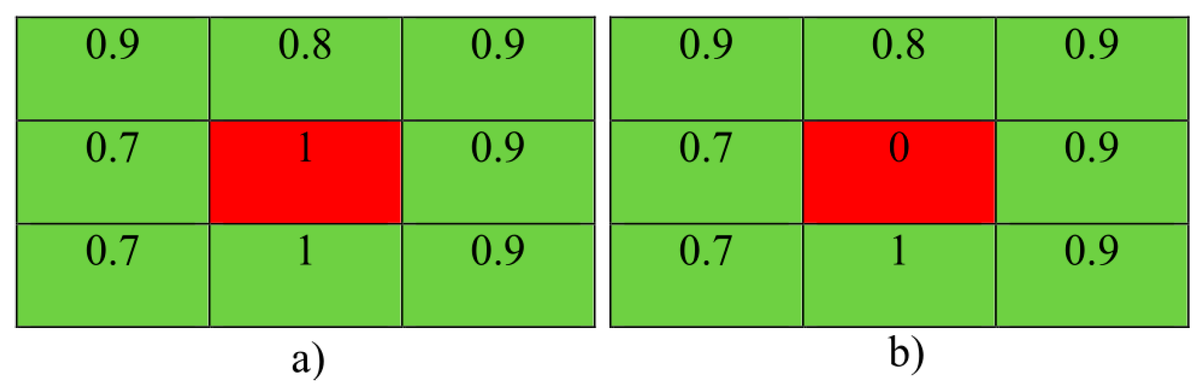
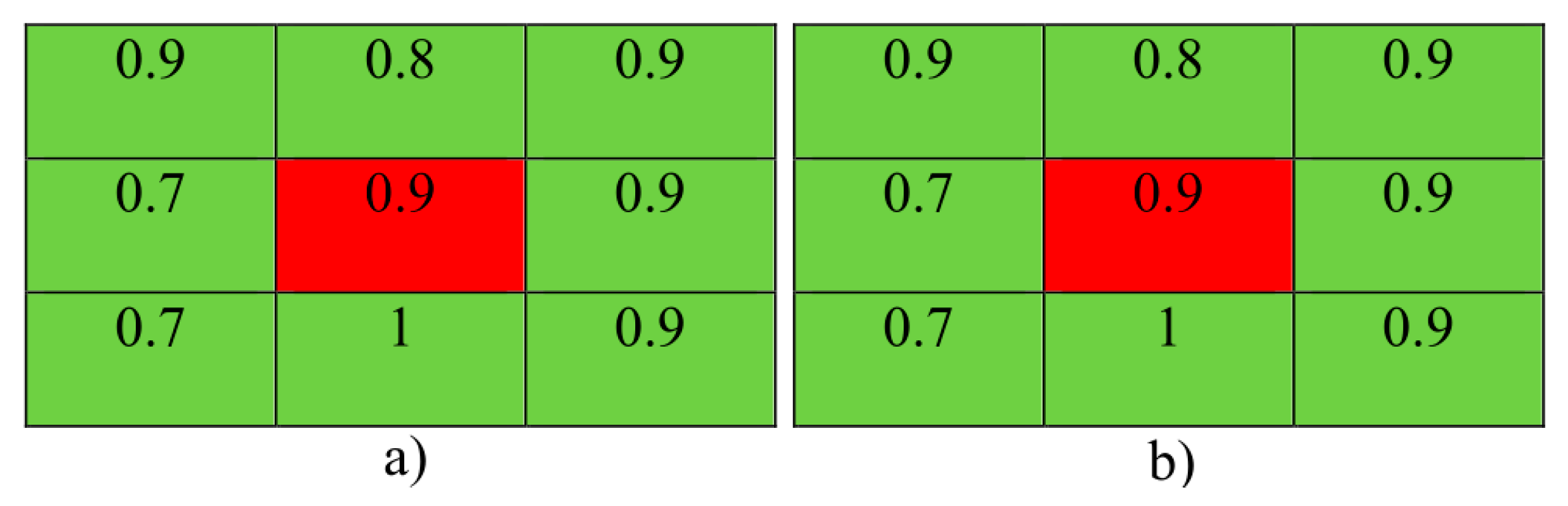
3.5. Local Statistical Aggregation
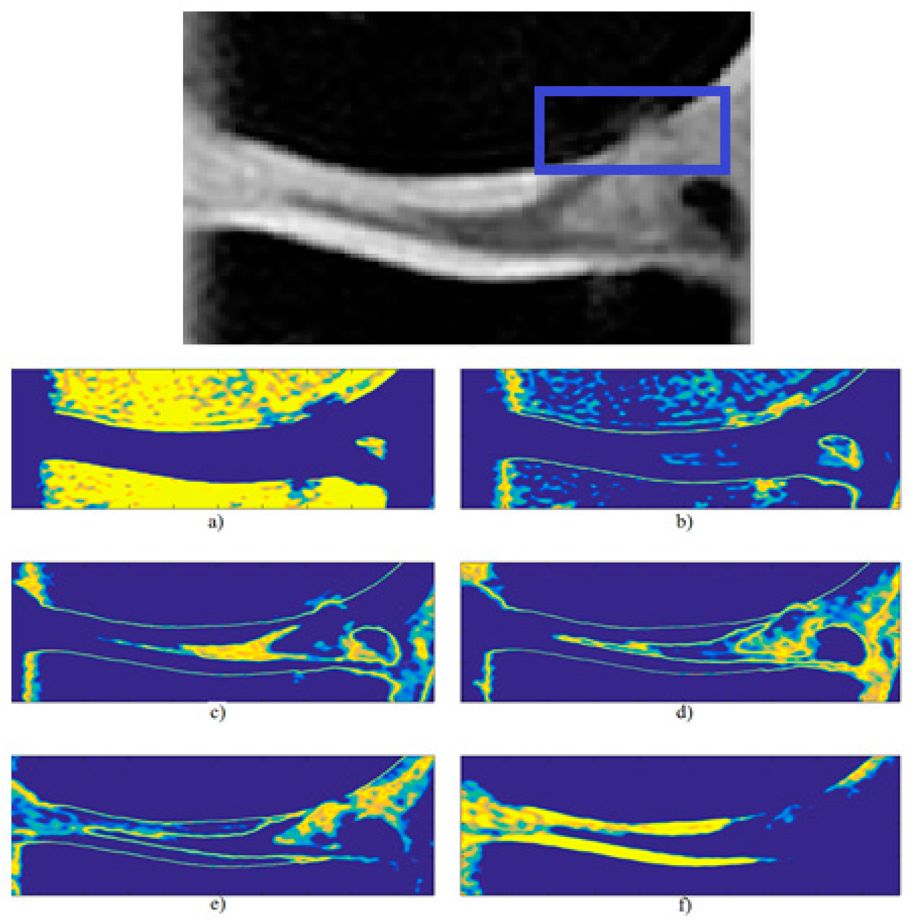
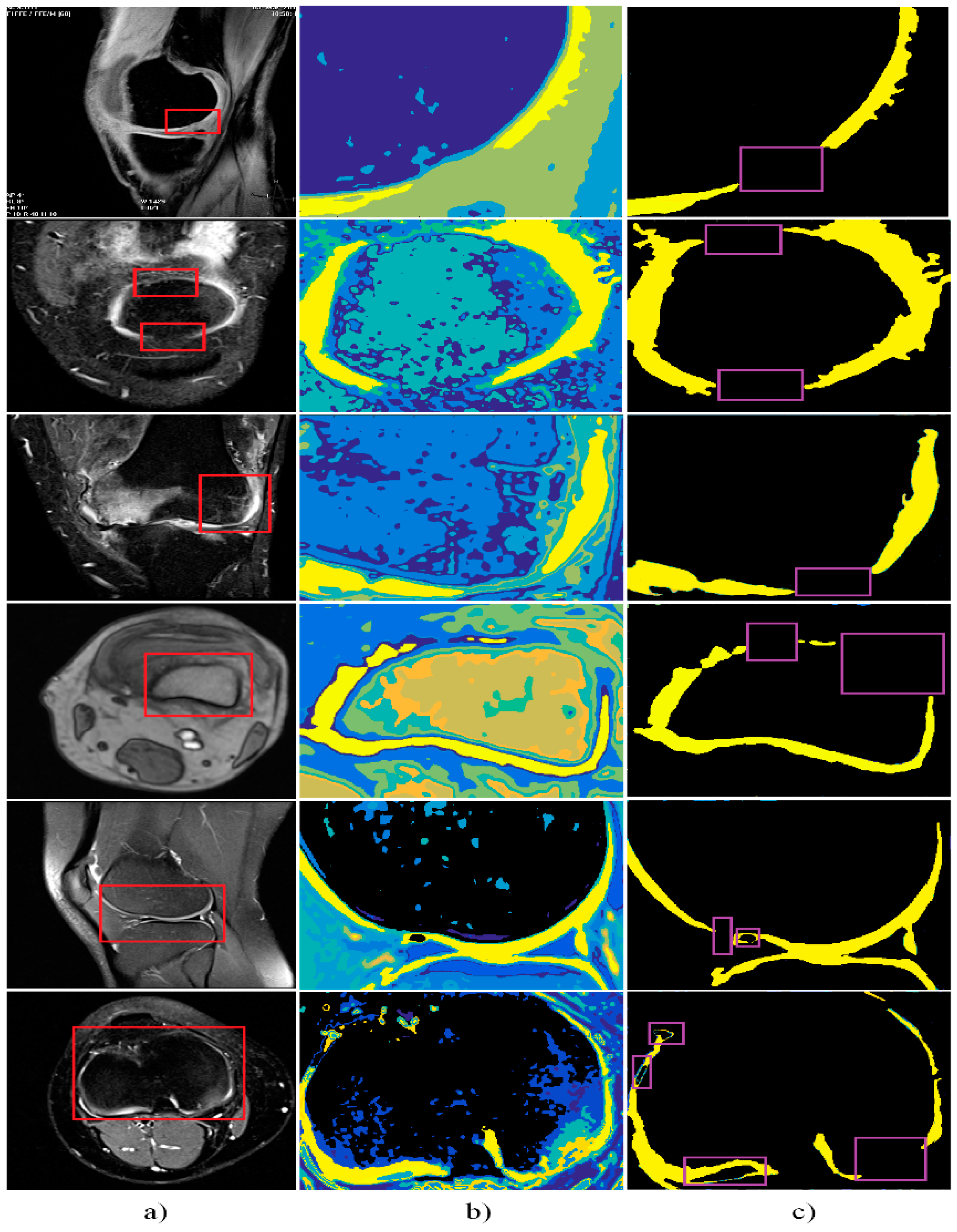
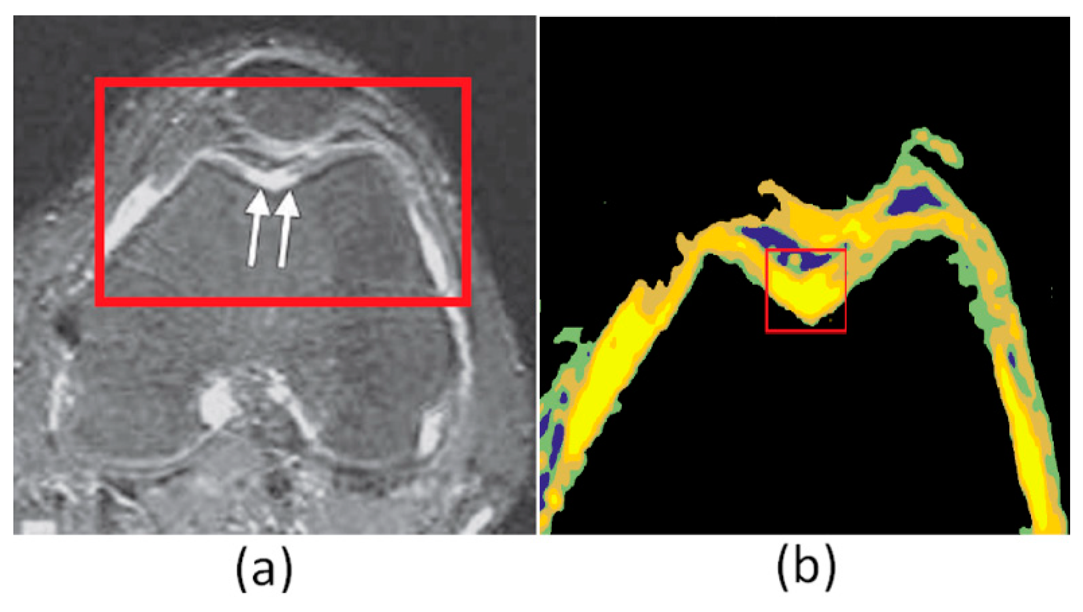
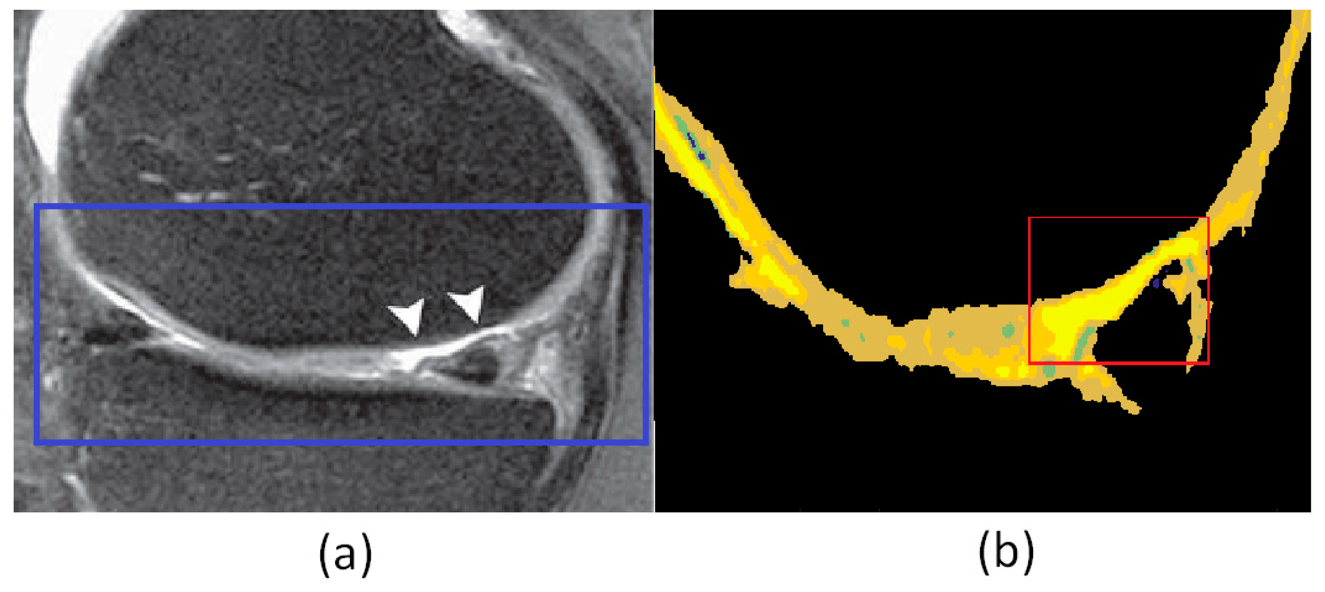
Intensity soft segmentation may lack of robustness, especially when the noisy pixels are present. It is supposed that the pixels representing the image noise have significantly different intensity in regards to pixels belonging to the articular cartilage area. This fact often leads to the incorrect classification of the noisy pixels, and the articular cartilage area contains so called blind spots deteriorating the structure of the cartilage model.
In the cartilage model, we use a local statistical aggregation scanning the membership values of all the pixels. By considering local statistical features of each segmentation region, the originally assigned membership values may be modified, and pixels may be re-classified, depending on the statistical features of the surrounding pixels.
Supposing we define for k pixel its neighborhood η(k), for such area we can consider local statistical features. In our model we use the median aggregation defined as follow:
μ l s ( I ( k ) ) = m e d i a n s η ( k ) { μ ( I ( s ) ) }
In the comparison with the average value, the median is invariant in a presence of outliers. Such pixels often represent the image noise, deteriorating the segmentation results. With the median as 50% quantile can reliably approximate the mean value, even if the noise is present. We suppose that the median represents a robust position parameter being invariant against the distant observations. Robustness ensures an effective using for the spatial segmentation which should not be affected by deviating membership values, with the goal of maximization of the segmentation efficiency, especially when the image noise is presented. The local aggregation is implemented by using the cyclic convolution with the kernel η(k), going through all the segmentation regions. We report an example of using the median aggregation (Figure 9) for pixel’s neighborhood of eight pixels.
It is obvious when not supposing a presence of the noisy pixels, all the pixels will have great membership values for respective region (Figure 9a). When noise is presented by the centered pixel, indicated as red (Figure 9b), such pixel has a significantly lower membership value for a respective region, when comparing with surrounding pixels, due to its different intensity features which can be expected in the image noise. The median local aggregation has the task to modify the originally assigned membership in a dependence of the pixel’s surrounding. If the analyzed pixels have similar intensity values, the median aggregation does not rapidly change them, contrarily the noise pixels membership may be substantially modified when considering their surroundings. Such a situation is illustrated in Figure 10 where we report an application of the median aggregation for the situation from Figure 9.

4. Results

The main intention of the proposed model is a proper localization of the healthy articular cartilage, with regard to the early stage of the cartilage loss caused by the osteoarthritis. MR imaging enables a reliable and contrast visualization of the healthy cartilage nevertheless the early pathological changes are often difficult to recognize by naked eyes.
We did the cartilage modeling on two issues. The first mentioned alternative deals with a selection of the region of the interest where the segmentation procedure is consequently applied. A certain disadvantage of this approach is a spatial limitation of the articular cartilage when only a part of the cartilage is subjected to the segmentation analysis. The second alternative deals with the analysis of the whole knee area where the cartilage is relatively small. In Figure 11, we report the example of the segmentation procedure applied on the MR image, containing the early cartilage loss, which is difficult to observe by naked eyes. We marked the analyzed cartilage area as red, and the early cartilage loss as violet in the segmentation model. The proposed segmentation model enables a differentiation between the physiological cartilage structure, indicated as yellow and the early cartilage loss, which is recognizable as the interruption between the healthy cartilage structures. For testing parameters of the ABC: Number of food sources (i = 100) and number of iterations (NI = 200).
One of the segmentation procedure implementations is the analysis of time-inverse knee images, which are evaluated for instance for the reason of presence the focal defects (Figure 12a), where the focal defect is manifested on the trochlear socket. The red RoI is segmented with eight classes and aggregated by the median window with size 9 × 9 pixels. In the Figure 12b, we present the resulting cartilage model.
Next, we tested the segmentation procedure in sagittal 2D SE images. Figure 13a represents the articular cartilage with the cartilage defect (arrows). The segmentation procedure differentiate the cartilage area (blue RoI), where other knee structures are suppressed.
One type of the articular cartilage morphological assessment is FLASH imaging. This technique is also usable for evaluation of time change of the cartilage thickness and volume. The physiological cartilage characterized by high signal intensity in the FLASH imaging. For this reason, the superficial lesions are better observable in deeper contrast. On the other hand, such lesions may be incorrectly jointed with the cartilage defects, for instance fissures. In the following output (Figure 14), we present the cartilage model, reflecting the complete cartilage loss of medial area with the degenerative lesions.
The last application, where we tested the proposed segmentation methodology is the MR imaging with variable force fields. These modalities are not conventionally used, but they are mostly used in an area of the clinical research. The main benefit of stronger magnetic fields is in contrast imaging of the articular cartilage. On the other hand, there is worse magnetic susceptibility in tissues, and images are more inclinable to the flow artefacts. Based on the studies, using the 7.0T MR imaging this modality is more effective for imaging of the morphological structure of the articular cartilage. The benefit of this imaging is achieving a better resolution, with a shorter acquisition time, when comparing with the 3.0T systems.
The following results shows application possibilities of the articular cartilage modeling from 3.0T (Figure 15) and 7.0T MR images (Figure 16). Analyzed data shows, in both cases, the physiological cartilage, which is represented by a higher level of the MR signal, which leads to a better contrast in comparison with adjacent tissues. The first important aspect in homogeneousness of the cartilage, which is, in the segmentation models, accompanied mostly by unified color spectrum (yellow spectrum). An important aspect of the segmentation model is also a robustness against the artefacts, caused by the magnetic field. The 7.0T image data are affected by the magnetic susceptibility, this phenomenon is indicated by arrows (Figure 16), nevertheless, this artefact is eliminated in the model.

5. Quantitative Comparison and Segmentation Performance

This section is dedicated to the quantitative testing and evaluation of the proposed segmentation model. The testing was done based the gold standard cartilage segmentation, defined by the clinical experts from the orthopedics (Figure 17), and against selected regional segmentation methods. In the second part of the testing, we evaluated optimal settings of the local aggregation for the cartilage segmentation. The gold standard images for the comparison were done by manual tracing of the cartilage boarders by clinical experts, having the attestation from orthopedics.
Firstly, we present a comparative analysis against some conventional segmentation methods. For this task, we consider methods based on the fuzzy approach, as well as the methods taking into account the spatial information. These methods are considered as significantly representative for the comparison.
  • Otsu thresholding (Otsu-N): Hard thresholding segmentation utilizing image partitioning into N regions.
  • Fuzzy C means (FCM): Represents clustering. An algorithm generates clusters into c parts, attempts to find centroids of natural clusters in the data. For this task, a minimization of the inner clustering variance based on error function is used.
  • Iterative thresholding (ITS): The initial thresholding is iteratively adjusted based on the local information and the resulting threshold is less sensitive against the noise.
  • Maximal Spatial Probability (MASP): It is a segmentation, considering the spatial information. A probability of pixel’s belonging to respective class, in a frame of spatial restrictions, is defined as spatial probability.
The following scalar metrics are used for the quantitative comparison:
Rand Index (RI): Measures a similarity between two segmentation regions. RI compares the compatibility of an assignment between pairs of elements in two regions. The RI formulation is as follows:
RI ( C 1 , C 2 ) = 2 n 11 + n 00 N ( N 1 )
where N stands for number of pixels, n 11 denotes a number of pairs belonging to the same area C 1 and C 2 , and n 00 stands for a number of pairs in different segmentation classes. RI gives values 0–1 where 0 indicates completely dissimilar regions and 1 stands for exactly same data.
Variation Information (VI): measures distance between two segmentations in a sense of their conditional entropy, which is defined:
VI ( C 1 ,   C 2 ) = ( C 1 ) + ( C 2 ) 2 I ( C 1 ,   C 2 )
where ( C i ) represents an entropy associated with the Ci and I is a mutual information between C 1 and C 2 .
Segmentation Overlapping: overlapping C 1 by C 2 is defined as follows:
C ( S 2 S 1 ) = 1 N R 1 S 1 | R 1 | max R 2 S 2 O ( R 1 , R 2 )  
where O ( R 1 , R 2 ) is an overlapping between the regions R 1 and R 2 defined as follows:
O ( R 1 , R 2 ) = | R 1 R 2 | R 1 R 2
We used two complementary descriptors: C ( S 2 S 1 ) and C ( S 1 S 2 ) .
We did testing for 100 MR image records where cartilage was extracted. Averaged results of native images (Nat), as well as additive Gaussian (Gauss) and multiplicative Rayleight (Mult) noise of all the tests are summarized in the Table 4. The best result, for each test, are highlighted. For each MR image, the gold standard was generated (Figure 17) by using the manual segmentation by clinical expert from the orthopedics.
We tested two alternatives of the proposed soft multiregional segmentation, differing in the local aggregation: Median (MedAg) and average (AvAg) aggregation. The greater values of RI and C we give, the better result of test we obtain, while the lower VI is, the better results we obtain. The reported results in the Table 4 show that the proposed method gives the best, and the most robust results, when comparing with other considered methods, even in the noisy environment represented by the Gaussian and multiplicative noise. When analyzing only the proposed method with different aggregators, we mostly get better results for the median aggregation. This fact is predictable regarding the fact that median represents a robust estimator of position.
In the next step, we compared the median aggregation with a different number of the segmentation classes (Figure 18). When selecting a higher number of the segmentation classes, the knee segmentation model (blue contour) contains tiny pixels clusters, especially in the femoral bone area, as well as the cartilage is severed. Contrarily, when selecting a lower number of clusters, the early cartilage loss is badly detectable in the model, due to a lower sensitivity.
The next important aspect of the testing is the robustness against the additive image noise. We report results of this testing for MR image RoI 500 × 400 pixels. Analysis is done for the additive image noise salt and pepper (Figure 19), additive Gaussian (Figure 20), and multiplicative Rayleight noise (Figure 21).
The proposed method was tested for deterministic noise reported in Figure 19, Figure 20, and Figure 21 for variable noise settings from softer deterioration of the intensity distribution, up to the cases where the intensity information completely missing. Based on the comparison, the proposed method gives the most robust results for the multiplicative noise. In this case, the shape parameters of the articular cartilage are mostly perceived. Contrarily, it is apparent that the proposed method is the most sensitive when the Gaussian noise is presented. Despite the cartilage contour smoothness being perceived, the main observable fact is the discontinuity of the cartilage structure where the cartilage loss is not nearly recognizable.
The last tested parameter of the segmentation procedure is the size of the median aggregation window. Based on the pixel’s surrounding, pixel’s membership may be re-considered. Based on the experimental results, the median aggregation appears as the most effective. Nevertheless, the size of the aggregation window has significant impact on the segmentation effectivity. The greater aggregation window is selected, the more pixels in neighborhood are considered. In order to clarify this situation, we report the comparative analysis for different aggregation settings of the aggregation (Figure 22).
The aggregation procedure gives a different smoothness of the segmentation classes, depending on the aggregation kernel size. When selecting the 3-square kernel (Figure 22a), the segmentation result gives a relatively higher proportion of the noisy clusters in the femoral bone area (blue contour). Contrarily, when selecting the greatest size 15-square of the median kernel (Figure 22d) these artifacts are nearly eliminated. Nevertheless, when selecting a higher kernel size, the cartilage is reduced. Such a fact underestimates the effect of the segmentation procedure. This fact is well represented in the Figure 23, indicated as red RoI.

6. Discussion

The articular cartilage diagnosis is one of the key procedures in the clinical practice of the orthopedics. Therefore, a proper evaluation of the morphological cartilage features, with regards to the early pathological changes is important. The MR imaging represents a current standard for the cartilage imaging due to a high spatial resolution and optimization of the imaging by using variable MR sequences. Despite all these benefits, the early cartilage loss, predicting a severe development of the cartilage deterioration, is badly recognizable from the native MR images. For this reason, a development of fully automatic method allowing for the identification and quantification of the physiological cartilage, and early cartilage loss is still challenging issue.
The proposed segmentation model utilizes a histogram partitioning based on a sequence of the triangular fuzzy sets. Conventional fuzzy thresholding enables a definition of the fuzzy model based on the centroids calculated by the clustering. Clustering usually requires initialization which influences clusters accuracy. This fact is a limitation for a proper distribution of the intensity segmentation. In the proposed approach, we performed the fuzzy thresholding model driven by the evolutionary optimization, based on the modified ABC algorithm, taking advantage the real cartilage features. Optimization method, in comparison with clustering, generates multiple solutions for the fuzzy set placement, where each of them is evaluated by using the fitness function within the segmentation. Furthermore, the proposed method is able to identify the respective class, representing the articular cartilage. This intensity segmentation is consequently completed by the local spatial aggregation. In the articular cartilage model, we use the median square kernel window which appears, based on the quantitative testing, as the most robust for both the native MR images and images corrupted by deterministic noise.
In the future, we are going to focus on the cartilage features extraction based on the proposed model. There are two challenging issues. Determining cartilage features, including the cartilage thickness and volumetric parameters enable to evaluate condition of the articular cartilage and they also serve as predictors for objectification of the cartilage deterioration. Since the proposed segmentation model is able to classify the physiological cartilage from the early cartilage loss, it would be worth measuring quantification of this impairment. This model feature would be able to objectivize a cartilage damage level.

Author Contributions

Conceptualization, D.O.; formal analysis, M.P. and M.A.; funding acquisition, M.P.; investigation, J.K.; methodology, J.K.; project administration, M.C. and J.K.; resources, M.P.; software, M.P.; supervision, J.K.; validation, D.O. and J.K.; visualization, M.A.; writing—original draft, J.K. and D.O.; writing—review and editing, J.K., M.C. and M.P.

Acknowledgments

This paper was supported by project No. CZ.02.1.01/0.0/0.0/17_049/0008441 “Innovative Therapeutic Methods of Musculoskeletal System in Accident Surgery” within the Operational Programme Research, Development and Education financed by the European Union and by the state budget of the Czech Republic. The work and the contributions were supported by the project SV4508811/2101Biomedical Engineering Systems XIV’. This study was also supported by the research project The Czech Science Foundation (GACR) 2017 No. 17-03037S Investment evaluation of medical device development run at the Faculty of Informatics and Management, University of Hradec Kralove, Czech Republic. This study was supported by the research project The Czech Science Foundation (TACR) ETA No. TL01000302 Medical Devices development as an effective investment for public and private entities.

Conflicts of Interest

The authors of the paper declare that do not have any conflict of interest.

References

  1. Hayashi, D.; Roemer, F.W.; Jarraya, M.; Guermazi, A. Imaging of osteoarthritis. In Geriatric Imaging; Springer: Berlin/Heidelberg, Germany, 2013. [Google Scholar] [CrossRef]
  2. Felson, D.T.; Niu, J.; Gross, K.D.; Englund, M.; Sharma, L.; Cooke, T.D.V.; Guermazi, A.; Roemer, F.W.; Segal, N.; Nevitt, M.C. Valgus malalignment is a risk factor for lateral knee osteoarthritis incidence and progression: Findings from the multicenter osteoarthritis study and the osteoarthritis initiative. Arthritis Rheum. 2013, 65, 355–362. [Google Scholar] [CrossRef] [PubMed]
  3. Link, T.M. MR imaging in osteoarthritis: Hardware, coils, and sequences. Radiol. Clin. 2009, 474, 617–632. [Google Scholar] [CrossRef] [PubMed]
  4. Guermazi, A.; Hayashi, D.; Roemer, F.W.; Felson, D.T. Osteoarthritis: A review of strengths and weaknesses of different imaging options. Rheum. Dis. Clin. 2013, 39, 567–591. [Google Scholar] [CrossRef] [PubMed]
  5. Park, H.J.; Kim, S.S.; Lee, S.Y.; Park, N.H.; Park, J.Y.; Choi, Y.J.; Jeon, H.J. A practical MRI grading system for osteoarthritis of the knee: Association with Kellgren-Lawrence radiographic scores. Eur. J. Radiol. 2013, 82, 112–117. [Google Scholar] [CrossRef] [PubMed]
  6. Li, X.; Pedoia, V.; Kumar, D.; Rivoire, J.; Wyatt, C.; Lansdown, D.; Amano, K.; Okazaki, N.; Savic, D.; Koff, M.F.; et al. Cartilage T 1ρ and T 2 relaxation times: Longitudinal reproducibility and variations using different coils, MR systems and sites. Osteoarthr. Cartil. 2015, 23, 2214–2223. [Google Scholar] [CrossRef] [PubMed]
  7. Shelbourne, K.D.; Urch, S.E.; Gray, T.; Freeman, H. Loss of normal knee motion after anterior cruciate ligament reconstruction is associated with radiographic arthritic changes after surgery. Am. J. Sports Med. 2012, 40, 108–113. [Google Scholar] [CrossRef] [PubMed]
  8. Hunter, D.J.; Arden, N.; Conaghan, P.G.; Eckstein, F.; Gold, G.; Grainger, A.; Zhang, W. Definition of osteoarthritis on MRI: Results of a Delphi exercise. Osteoarthr. Cartil. 2011, 19, 863–969. [Google Scholar] [CrossRef]
  9. Sheehy, L.; Culham, E.; McLean, L.; Niu, J.; Lynch, J.; Segal, N.A.; Cooke, T.D.V. Validity and sensitivity to change of three scales for the radiographic assessment of knee osteoarthritis using images from the Multicenter Osteoarthritis Study (MOST). Osteoarthr. Cartil. 2015, 23, 1491–1498. [Google Scholar] [CrossRef] [PubMed] [Green Version]
  10. Stefanik, J.J.; Guermazi, A.; Zhu, Y.; Zumwalt, A.C.; Gross, K.D.; Clancy, M.; Felson, D.T. Quadriceps weakness, patella alta, and structural features of patellofemoral osteoarthritis. Arthr. Care Res. 2011, 63, 1391–1397. [Google Scholar] [CrossRef] [PubMed]
  11. Braun, H.J.; Gold, G.E. Diagnosis of osteoarthritis: Imaging. Bone 2012, 51, 278–288. [Google Scholar] [CrossRef]
  12. Boesen, M.; Ellegaard, K.; Henriksen, M.; Gudbergsen, H.; Hansen, P.; Bliddal, H.; Riis, R.G. Osteoarthritis year in review 2016: Imaging. Osteoarthr. Cartil. 2017, 25, 216–226. [Google Scholar] [CrossRef] [PubMed]
  13. Wenham, C.Y.J.; Grainger, A.J.; Conaghan, P.G. The role of imaging modalities in the diagnosis, differential diagnosis and clinical assessment of peripheral joint osteoarthritis. Osteoarthr. Cartil. 2014, 22, 1692–1702. [Google Scholar] [CrossRef] [PubMed] [Green Version]
  14. Trattnig, S.; Winalski, C.S.; Marlovits, S.; Jurvelin, J.S.; Welsch, G.H.; Potter, H.G. Magnetic resonance imaging of cartilage repair: A review. Cartilage 2011, 2, 5–26. [Google Scholar] [CrossRef] [PubMed]
  15. Kijowski, R.; Blankenbaker, D.G.; Munoz del Rio, A.; Baer, G.S.; Graf, B.K. Evaluation of the Articular Cartilage of the Knee Joint: Value of adding a T2 mapping sequence to a routine mr imaging protocol. Radiology 2013, 267, 503–513. [Google Scholar] [CrossRef] [PubMed]
  16. Guermazi, A.; Roemer, F.W.; Alizai, H.; Winalski, C.S.; Welsch, G.; Brittberg, M.; Trattnig, S. State of the art: MR imaging after knee cartilage repair surgery. Radiology 2015, 277, 23–43. [Google Scholar] [CrossRef]
  17. Ho-Fung, V.M.; Jaramillo, D. Cartilage imaging in children. Current indications, magnetic resonance imaging techniques, and imaging findings. Radiol. Clin. N. Am. 2013. [Google Scholar] [CrossRef]
  18. Jungmann, P.M.; Baum, T.; Bauer, J.S.; Karampinos, D.C.; Erdle, B.; Link, T.M.; Welsch, G.H. Cartilage repair surgery: Outcome evaluation by using noninvasive cartilage biomarkers based on quantitative mri techniques? BioMed Res. Int. 2014. [Google Scholar] [CrossRef]
  19. Suppanee, R.; Yazdifar, M.; Chizari, M.; Esat, I.; Bardakos, N.V.; Field, R.E. Simulating osteoarthritis: The effect of the changing thickness of articular cartilage on the kinematics and pathological bone-to-bone contact in a hip joint with femoroacetabular impingement. Eur. Orthop. Traumatol. 2014, 5, 65–73. [Google Scholar] [CrossRef]
  20. Wu, Y.; Krishnan, S.; Rangayyan, R.M. Computer-aided diagnosis of knee-joint disorders via vibroarthrographic signal analysis: A review. Crit. Rev. TM Biomed. Eng. 2012, 38. [Google Scholar] [CrossRef]
  21. Eckstein, F.; Glaser, C. Measuring cartilage morphology with quantitative magnetic resonance imaging. Semin. Musculoskelet. Radiol. 2004. [Google Scholar] [CrossRef]
  22. Lee, K.Y.; Dunn, T.C.; Steinbach, L.S.; Ozhinsky, E.; Ries, M.D.; Majumdar, S. Computer-aided quantification of focal cartilage lesions of osteoarthritic knee using MRI. Magn. Reson. Imaging 2004, 22, 1105–1115. [Google Scholar] [CrossRef] [PubMed]
  23. Dam, E.B.; Folkesson, J.; Pettersen, P.C.; Christiansen, C. Semi-automatic knee cartilage segmentation. Prog. Biomed. Opt. Imaging—Proc. SPIE 2006, 6144, 614441. [Google Scholar]
  24. Görres, J.; Brehler, M.; Franke, J.; Vetter, S.Y.; Grützner, P.A.; Meinzer, H.-P.; Wolf, I. Articular surface segmentation using active shape models for intraoperative implant assessment. Int. J. Comput. Assist. Radiol. Surg. 2016, 11, 1661–1672. [Google Scholar] [CrossRef] [PubMed]
  25. Tabrizi, P.R.; Zoroofi, R.A.; Yokota, F.; Nishii, T.; Sato, Y. Shape-based acetabular cartilage segmentation: Application to CT and MRI datasets. Int. J. Comput. Assist. Radiol. Surg. 2016, 11, 1247–1265. [Google Scholar] [CrossRef] [PubMed]
  26. Tabrizi, P.R.; Zoroofi, R.A.; Yokota, F.; Tamura, S.; Nishii, T.; Sato, Y. Acetabular cartilage segmentation in CT arthrography based on a bone-normalized probabilistic atlas. Int. J. Comput. Assist. Radiol. Surg. 2015, 10, 433–446. [Google Scholar] [CrossRef] [PubMed]
  27. Fripp, J.; Crozier, S.; Warfield, S.K.; Ourselin, S. Automatic segmentation and quantitative analysis of the articular cartilages from magnetic resonance images of the knee. IEEE Trans. Med. Imaging 2010, 29, 55–64. [Google Scholar] [CrossRef] [PubMed]
  28. Kumarv, A.; Jayanthy, A.K. Classification of MRI images in 2D coronal view and measurement of articular cartilage thickness for early detection of knee osteoarthritis. In Proceedings of the 2016 IEEE International Conference on Recent Trends in Electronics, Information and Communication Technology (RTEICT 2016), Bangalore, India, 20–21 May 2016; pp. 1907–1911. [Google Scholar]
  29. Kubicek, J.; Penhaker, M.; Augustynek, M.; Bryjova, I.; Cerny, M. Segmentation of Knee Cartilage: A Comprehensive Review. J. Med. Imaging Health Inform. 2018, 8, 401–418. [Google Scholar] [CrossRef]
  30. Gougoutas, A.J.; Wheaton, A.J.; Borthakur, A.; Shapiro, E.M.; Kneeland, J.B.; Udupa, J.K.; Reddy, R. Cartilage volume quantification via Live Wire segmentation. Acad. Radiol. 2004, 11, 1389–1395. [Google Scholar] [CrossRef]
  31. Mikulka, J.; Gescheidtova, E.; Bartusek, K. Modern edge-based and region-based segmentation methods. In Proceedings of the TSP 2009—32nd International Conference on Telecommunications and Signal Processing, Dunakiliti, Hungary, 26 August 2009; pp. 89–91. [Google Scholar]
  32. Kubicek, J.; Vicianova, V.; Penhaker, M.; Augustynek, M. Time deformable segmentation model based on the active contour driven by Gaussian energy distribution: Extraction and modeling of early articular cartilage pathological interuptions. Front. Artif. Intell. Appl. 2017, 297, 242–255. [Google Scholar]
  33. Aja-Fernández, S.; Curiale, A.H.; Vegas-Sánchez-Ferrero, G. A local fuzzy thresholding methodology for multiregion image segmentation. Knowl.-Based Syst. 2015, 83, 1–12. [Google Scholar] [CrossRef]
  34. Ma, M.; Liang, J.; Guo, M.; Fan, Y.; Yin, Y. SAR image segmentation based on artificial bee colony algorithm. Appl. Soft Comput. J. 2011, 11, 5205–5214. [Google Scholar] [CrossRef]
  35. Horng, M.H. Multilevel thresholding selection based on the artificial bee colony algorithm for image segmentation. Expert Syst. Appl. 2011, 38, 13785–13791. [Google Scholar] [CrossRef]
  36. Sağ, T.; Çunkaş, M. Color image segmentation based on multiobjective artificial bee colony optimization. Appl. Soft Comput. J. 2015, 34, 389–401. [Google Scholar] [CrossRef]
  37. Osuna-Enciso, V.; Cuevas, E.; Sossa, H. A comparison of nature inspired algorithms for multi-threshold image segmentation. Expert Syst. Appl. 2013, 40, 1213–1219. [Google Scholar] [CrossRef] [Green Version]
Figure 1. Clinical cases of the MR knee cartilage visualization, including the early cartilage loss, indicated as red marked circles.
Symmetry 11 00861 g001
Figure 2. A complex structure of the proposed methodology of segmentation and cartilage modeling.
Symmetry 11 00861 g002
Figure 3. A sequence of individual triangular functions specifying individual image regions.
Symmetry 11 00861 g003
Figure 4. Native MR knee image with active contour model detecting the physiological femoral cartilage (left), energy map of the active contour (middle), and a binary model of the physiological cartilage (right).
Symmetry 11 00861 g004
Figure 5. An example of optimization of V k segmentation class.
Symmetry 11 00861 g005
Figure 6. A complex structure for soft methodology optimization based on the modified artificial bee colony (ABC) algorithm.
Symmetry 11 00861 g006
Figure 7. Convergence characteristics for the fitness function evolution within 100 iterations: (a) 100 food sources and (b) 50 food sources.
Symmetry 11 00861 g007
Figure 8. Extract of native MR image, containing the articular cartilage, with the osteoarthritis change, indicated by the blue RoI. A sequence of individual segmentation models of the articular cartilage by using 6 segmentation classes is represented by (af). The color spectrum differentiates a level of individual tissue membership. Yellow color represents presence of individual tissue, while blue color identifies the background (non-presence) of the respective tissue.
Symmetry 11 00861 g008
Figure 9. Neighborhood of analyzed pixel, indicated as red where: (a) it is not supposed a presence of the noisy pixels and (b) analyzed centered pixel represents the image noise.
Symmetry 11 00861 g009
Figure 10. Application of the local median aggregation for: (a) pixels not containing the image noise and (b) noisy centered pixel.
Symmetry 11 00861 g010
Figure 11. Example of cartilage segmentation model: (a) Native MR knee images, containing the early cartilage loss where the cartilage area is indicated as red, (b) proposed soft segmentation model with 8 classes—cartilage is shown by yellow contour, and (c) extraction of the articular cartilage where the violet RoI indicate the cartilage interruptions caused by the early cartilage loss.
Symmetry 11 00861 g011
Figure 12. Time-inverse knee image (a), indicating the full chondral defect (arrows), with marked RoI for segmentation, and segmentation model (eight segmentation classes) of the time-inverse knee image after region of articular cartilage extraction (b), where the focal defect is sharply indicated in red RoI. Artificial colors represent segmentation classes in the cartilage, according to the MR signal strength and other knee tissues are suppressed.
Symmetry 11 00861 g012
Figure 13. The native data of the knee area (a), obtained by 2D SE imaging. The native image gives a better contrast between the cartilage surface and synovial fluid. A high contrast well differentiate cartilage defect (arrows), where the blue RoI indicates the area of the interest for segmentation. The segmentation model (b) identifies a part of the cartilage region, where the cartilage defect is sharply indicated by yellow contour in the red RoI.
Symmetry 11 00861 g013
Figure 14. T2 weighted image with fat suppression (a) reflects locations of the complete cartilage loss in medial tibia-femoral area with degenerative lesions in the subchondral bone (arrows), where red RoI indicates area of the interest for segmentation procedure. The segmentation model (b) of the articular cartilage, reflecting the highest signal intensity (yellow contours), contrarily model detects the locations of the cartilage loss (red areas of interest), degenerative lesions are sharply indicated by yellow contour in the blue RoI.
Symmetry 11 00861 g014
Figure 15. Sagittal 3.0T MR image of knee area of healthy volunteer, not exhibiting significant differences in manifestation of the articular cartilage (a) and cartilage segmentation model (b), identifying the morphological structure homogeneity (yellow contour).
Symmetry 11 00861 g015
Figure 16. Sagittal 7.0T MR image of the knee area of healthy volunteer, not exhibiting significant differences in manifestation of the articular cartilage (a). The native data contain artefacts, caused by the magnetic susceptibility (arrows). The segmentation model of the articular cartilage (b) identifies the morphological structure compactness (yellow contour).
Symmetry 11 00861 g016
Figure 17. Example of the gold standard definition by tracing the articular cartilage by clinical expert: (a) manual tracing of the femoral cartilage and (b) binary model of the cartilage.
Symmetry 11 00861 g017
Figure 18. A comparison of the cartilage segmentation applied on image region of the interest (RoI) 250 × 200 px: (a) 3, (b) 5, (c) 8, and (d) 12 classes.
Symmetry 11 00861 g018
Figure 19. Native results corrupted by the additive salt and pepper noise (up row) and segmentation results (down row) for noise density (d): (a) d 1 = 0.05 , (b) d 2 = 0.1 , (c) d 3 = 0.5 , and (d) d 4 = 0.8 .
Symmetry 11 00861 g019
Figure 20. Native results corrupted by the additive Gaussian noise (up row) and segmentation results (down row) for average value ( μ ) and dispersion ( σ 2 ): (a) μ = 0, σ 1 2 = 0.01, (b) μ = 0, σ 2 2 = 0.08, (c) μ = 0, σ 3 2 = 0.1, and (d) μ = 0, σ 4 2 = 0.8.
Symmetry 11 00861 g020
Figure 21. Native results corrupted by the multiplicative Rayleight noise (up row) and segmentation results (down row) for average value ( μ ) and dispersion ( σ 2 ): (a) μ = 0, σ 1 2 = 0.01, (b) μ = 0, σ 2 2 = 0.08, (c) μ = 0, σ 3 2 = 0.1, and (d) μ = 0, σ 4 2 = 0.8.
Symmetry 11 00861 g021
Figure 22. A comparison of different settings of median aggregation procedure on RoI 500 × 400 pixels, with square kernel: (a) 3, (b) 5, (c) 8, and (d) 15 pixels.
Symmetry 11 00861 g022
Figure 23. Median aggregation procedure with 23-square kernel where reduction of the cartilage structure is indicated by the red RoI.
Symmetry 11 00861 g023
Table 1. Comparison of interval estimations for articular cartilage.
Interval median estimation 209.54 ; 212.37
Gastwirth median estimation〈209.12; 211.95〉
Table 2. Extract of comparison fitness function of ABC optimization.
Testing ImageNumber of Classes f i t b e s t f i t w o r s t f i t m e d i a n f i t m e a n f i t S D
1621.4321.1121.4321.410.11
2622.6522.1422.3322.290.14
3622.4421.9922.1222.110.12
4622.1221.4421.9921.970.11
5621.9921.5421.6821.720.21
Table 3. Time complexity of soft segmentation.
Testing Image [px]Image OrderNumber of Classes Time Complexity [s]
(800 × 800)168.92
2610.54
3610.12
(300 × 300)169.91
269.11
368.59
(150 × 150)165.45
265.22
366.12
Table 4. Comparative analysis of quantitative evaluation of proposed of regional segmentation. (The bold font highlights the best results in the table.).
MedAgAvAgFCMOtsu-NITSMASP
RINat.0.7910.7280.7230.7230.7390.698
Gauss.0.6970.6690.6010.6830.6810.667
Mult.0.6810.6970.6650.6540.6120.571
VINat.2.9562.6112.9792.6752.9223.459
Gauss.3.1223.7883.3123.3673.1223.998
Mult.3.2333.8113.7113.5683.6793.799
C ( S 2 S 1 ) Nat.0.3660.3430.3540.3430.3710.219
Gauss.0.2980.3220.2910.2620.3120.242
Mult.0.3450.2890.2710.2330.3270.236
C ( S 1 S 2 ) Nat.0.4980.4480.4550.4110.4670.341
Gauss.0.4990.2950.3530.4120.3990.277
Mult.0.3910.3650.3430.3670.3890.311

