N-Soliton Solutions for the NLS-Like Equation and Perturbation Theory Based on the Riemann–Hilbert Problem

Abstract

In this paper, a kind of nonlinear Schrödinger (NLS) equation, called an NLS-like equation, is Riemann–Hilbert investigated. We construct a $2\times 2$ Lax pair associated with the NLS equation and combine the spectral analysis to formulate the Riemann–Hilbert (R–H) problem. Then, we mainly use the symmetry relationship of potential matrix Q to analyze the zeros of $det{P}^{+}$ and $det{P}^{-}$; the N-soliton solutions of the NLS-like equation are expressed explicitly by a particular R–H problem with an unit jump matrix. In addition, the single-soliton solution and collisions of two solitons are analyzed, and the dynamic behaviors of the single-soliton solution and two-soliton solutions are shown graphically. Furthermore, on the basis of the R–H problem, the evolution equation of the R–H data with the perturbation is derived.

1. Introduction

It is known that soliton theory plays an important role in many fields. There are many methods to study soliton equations, of which the inverse scattering method [1,2,3] and the Riemann–Hilbert (R–H) method [4,5,6,7] are two important techniques. The former uses the nonlinear Fourier method [8], in which the calculation procedure is extremely complicated. Conversely, the latter can provide an equivalent and more direct method to solve integrable equations, especially for soliton solutions. Thus, this method has been constantly developed [9,10,11,12,13,14,15]. Furthermore, there are many techniques and transformations for finding exact solutions for soliton equations, such as the Darboux transformation method [16,17,18], the Bäcklund transformation method [19,20], the Hirota bilinear method [21,22,23], the homogeneous balance method [24,25], Frobenius integrable decompositions [26,27,28], and Wronskian technology [29,30]. These methods have greatly promoted the development of soliton theory. From the specific limit of the general soliton solution, lump solutions [31,32,33,34], periodic solutions [35,36], and complex solutions [37,38] can be obtained. In recent years, the initial value problem of integrable equations on the half-line and finite interval [39,40,41] have also been discussed by formulating an associated R–H problem.

As we all know, the soliton solutions of soliton equations with important physical backgrounds have been widely studied. Among them, the nonlinear Schrödinger (NLS) equation is a very significant integrable model in Mathematical physics, which describes water wave theory, nonlinear optics, plasma physics, and so on. It has the following form:

$$i{q}_t+q_{xx}\pm 2q{\left|q\right|}^2=0.$$

(1)

On the basis of this, an NLS-like equation

$$i{q}_t+q_{xx}-{2q\left|q\right|}^2+{2a\left(\right|q|}^2{)}_{x}q=0,a\in \mathbb{R}$$

(2)

is derived as follows. We consider a soliton equation which has the following Lax pair:

$${\Phi }_x=M\Phi ,M=\left(\begin{array}{cc}-i{\lambda }^2& q\\ r& i{\lambda }^2\end{array}\right),$$

(3)

$${\Phi }_t=N_0\Phi ,N_0=\left(\begin{array}{cc}A& B\\ C& -A\end{array}\right),$$

(4)

where $\Phi (x,t,\lambda )$ is a matrix function, A, B, C contain the spectral parameter $\lambda$ and function q, r and its derivatives. The related stationary zero curvature equation is

$$N_{0x}=[M,N_0].$$

(5)

Then the Equation (5) becomes

$$\begin{array}{cc}\hfill A_x& =qC-Br,\hfill \\ \hfill B_x& =-2i{\lambda }^{2}B-2Aq,\hfill \\ \hfill C_x& =2i{\lambda }^{2}C+2Ar.\hfill \end{array}$$

(6)

Let us take A, B, C as the six polynomial of $\lambda$,

$$A=\sum _{j=0}^6{a}_j{\lambda }^j,B=\sum _{j=0}^6{b}_j{\lambda }^j,C=\sum _{j=0}^6{c}_j{\lambda }^j.$$

(7)

Therefore, the Equation (6) has following equivalence relation:

$$\begin{array}{c}{b}_6=c_6=0,a_{6x}=0,\hfill \\ a_{jx}=q{c}_j-b_{j}r,(j=0,1,2,3,4,5)\hfill \\ b_{j-2}=\frac{i}{2}{b}_{jx}+i{a}_{j}q,\hfill \\ c_{j-2}=-\frac{i}{2}{c}_{jx}+i{a}_{j}r.\hfill \end{array}$$

We choose $a_6=\alpha =\mathrm{const}$, and have

$$\begin{array}{c}{b}_4=\frac{i}{2}{b}_{6x}+i{a}_{6}q=i\alpha q,\hfill \\ c_4=-\frac{i}{2}{c}_{6x}+i{a}_{6}r=i\alpha r,\hfill \\ a_{4x}=q{c}_4-b_{4}r=iq\alpha r-iq\alpha r=0.\hfill \end{array}$$

The following equations can be obtained by setting $a_4=\beta =\mathrm{const}$:

$$\begin{array}{c}{b}_2=\frac{i}{2}{b}_{4x}+i{a}_{4}q=\frac{i}{2}{\left(i\alpha q\right)}_x+i\beta q=-\frac{\alpha }{2}{q}_x+i\beta q,\hfill \\ c_2=-\frac{i}{2}{c}_{4x}+i{a}_{4}r=-\frac{i}{2}{\left(i\alpha r\right)}_x+i\beta r=\frac{\alpha }{2}{r}_x+i\beta r,\hfill \\ a_{2x}=q{c}_2-b_{2}r=q(\frac{\alpha }{2}{r}_x+i\beta r)-(-\frac{\alpha }{2}{q}_x+i\beta q)r\hfill \\ =\frac{\alpha }{2}(q{r}_x+q_{x}r)=\frac{\alpha }{2}{\left(qr\right)}_x.\hfill \end{array}$$

In addition, we can get $a_2=\frac{\alpha }{2}qr+a_{20}$ ($a_{20}=\mathrm{const}$) and

$$\begin{array}{c}{b}_0=\frac{i}{2}{b}_{2x}+i{a}_{2}q=\frac{i}{4}\alpha (-q_{xx}+2q^{2}r)-\frac{1}{2}\beta q_x+iq{a}_{20},\hfill \\ c_0=-\frac{i}{2}{c}_{2x}+i{a}_{2}r=\frac{i}{4}\alpha (-r_{xx}+2q{r}^2)+\frac{1}{2}\beta r_x+ir{a}_{20},\hfill \\ a_{0x}=q{c}_0-b_{0}r=-\frac{i}{4}\alpha {(q{r}_x-r{q}_x)}_x+\frac{1}{2}\beta {\left(qr\right)}_x.\hfill \end{array}$$

Similarly, $a_0=-\frac{i}{4}\alpha (q{r}_x-r{q}_x)+\frac{1}{2}\beta qr+a_{00},(a_{00}=\mathrm{const})$ can be obtained. We also choose $b_5=c_5=0$, through the same steps as above and have $a_5=0,b_3=b_1=0,c_3=c_1=0$. Thus,

$$\begin{array}{c}A=a_6{\lambda }^6+a_5{\lambda }^5+a_4{\lambda }^4+a_3{\lambda }^3+a_2{\lambda }^2+a_1{\lambda }^1+a_0{\lambda }^0\hfill \\ =-\frac{i}{4}\alpha (q{r}_x-r{q}_x)+\frac{1}{2}\beta qr+a_{00}\hfill \\ +(\frac{\alpha }{2}qr+a_{20}){\lambda }^2+\beta {\lambda }^4+\alpha {\lambda }^6,\hfill \\ B=b_6{\lambda }^6+b_5{\lambda }^5+b_4{\lambda }^4+b_3{\lambda }^3+b_2{\lambda }^2+b_1{\lambda }^1+b_0{\lambda }^0\hfill \\ =\frac{i}{4}\alpha (-q_{xx}+2q^{2}r)-\frac{1}{2}\beta q_x+iq{a}_{20}\hfill \\ +(-\frac{\alpha }{2}{q}_x+i\beta q){\lambda }^2+\left(i\alpha q\right){\lambda }^4,\hfill \\ C=c_6{\lambda }^6+c_5{\lambda }^5+c_4{\lambda }^4+c_3{\lambda }^3+c_2{\lambda }^2+c_1{\lambda }^1+c_0{\lambda }^0\hfill \\ =\frac{i}{4}\alpha (-r_{xx}+2q{r}^2)+\frac{1}{2}\beta r_x+ir{a}_{20}\hfill \\ +(\frac{\alpha }{2}{r}_x+i\beta r){\lambda }^2+\left(i\alpha r\right){\lambda }^4.\hfill \end{array}$$

The matrix spectral problem can be obtained by taking $\alpha =a_{00}=a_{20}=0,\beta =-2i,r=-\overline{q}$,

$$\begin{array}{cc}\hfill M& =\left(\begin{array}{cc}-i{\lambda }^2& q\\ -\overline{q}& i{\lambda }^2\end{array}\right),\hfill \\ \hfill N_0& =\left(\begin{array}{cc}-2i{\lambda }^4+i{\left|q\right|}^2& i{q}_x+2{\lambda }^{2}q\\ i{\overline{q}}_x-2{\lambda }^2\overline{q}& 2i{\lambda }^4-i{\left|q\right|}^2\end{array}\right).\hfill \end{array}$$

A direct calculation shows $q_t-i{q}_{xx}-2iq{\left|q\right|}^2=0$. Notice that the term $-{2iq\left|q\right|}^2$ is independent of $\lambda$, thus, it can become positive as we assume

$$N_1=\left(\begin{array}{cc}-2i{\lambda }^4-i{\left|q\right|}^2& i{q}_x+2{\lambda }^{2}q\\ i{\overline{q}}_x-2{\lambda }^2\overline{q}& 2i{\lambda }^4+i{\left|q\right|}^2\end{array}\right),$$

and using the same method as above, we have

$$N=\left(\begin{array}{cc}-2i{\lambda }^4-i{\left|q\right|}^2+A_1& i{q}_x+2{\lambda }^{2}q+B_1\\ i{\overline{q}}_x-2{\lambda }^2\overline{q}+C_1& 2i{\lambda }^4+i{\left|q\right|}^2-A_1\end{array}\right).$$

The corresponding zero curvature equation is $M_t-N_x+[M,N]=0$, and we get

$$\left\{\begin{array}{c}{q}_t-i{q}_{xx}-B_{1x}+2iq{\left|q\right|}^2-2A_{1}q-2i{\lambda }^2{B}_1=0,\hfill \\ -{\overline{q}}_t-i{\overline{q}}_{xx}-C_{1x}+2i\overline{q}{\left|q\right|}^2-2A_1\overline{q}+2i{\lambda }^2{C}_1=0.\hfill \end{array}\right.$$

Taking $B_1=C_1=0,A_1={ia\left(\right|q|}^2{)}_x$, the $2\times 2$ Lax pair can be obtained:

$$\begin{array}{c}{\Phi }_x=M\Phi ,\hfill \\ M=\left(\begin{array}{cc}-i{\lambda }^2& q\\ -\overline{q}& i{\lambda }^2\end{array}\right),\hfill \end{array}$$

(8)

$$\begin{array}{c}\hfill {\Phi }_t=N\Phi ,\\ \hfill N=\left(\begin{array}{cc}-2i{\lambda }^4+{ia\left|q\right|}_x^2-i{\left|q\right|}^2& i{q}_x+2{\lambda }^{2}q\\ i{\overline{q}}_x-2{\lambda }^2\overline{q}& 2i{\lambda }^4-{ia\left|q\right|}_x^2+i{\left|q\right|}^2\end{array}\right),\end{array}$$

(9)

where the symbol $“-”$ represents complex conjugation. In our analysis, we assume the potential q is smooth enough and decays rapidly to zero when $x\to \pm \infty$. Furthermore, at any later time t, we look for solution $q(x,t)$ with the initial condition $q(x,0)$. When setting $a=0$, Equation (2) becomes a classical nonlinear Schrödinger Equation (1).

In this paper, we study the perturbation theory of the NLS-like equation. Obviously, small perturbations of integrable conditions can be regarded as perturbations of integrable models. Our formalism is in view of the R–H problem related to the NLS-like equation. The main advantage of the proposed method is its algebraic property, which is different from the method using the Gel’Fand Leviaon integral equation [42]. The R–H problem has many applications in dealing with disturbed soliton dynamics [43]. Modern versions of perturbation theory for the R–H problem have been published in a series of papers [44,45,46,47]. The direct perturbation theory is another form of soliton perturbation theory, which develops on the basis of the perturbation solution expansion into the square eigenfunction of the linearized soliton equation [48].

The main structure of this article is as follows. In Section 2, we give the Lax pair of the NLS-like equation. Then, the properties of the equivalent space matrix spectral problem of matrix eigenfunctions are analyzed, and the R–H problem related to the newly introduced space matrix spectral problem is formulated. In Section 3, through the special reductive R–H problem, in which the jump matrix is a unit matrix, the explicit expressions of the N-soliton solutions are obtained. In addition, the single soliton solution and collisions of the two-soliton solutions are analyzed. The perturbation theory based on Section 2 and the evolution equation of R–H data with perturbation are given in Section 4. Finally, the paper is summarized and further questions are given in Section 5.

2. The Riemann–Hilbert Problem

In what follows, we set $a=1$, and constructed a R–H formulation for Equation (2) with scattering and inverse scattering methods.

Let $T={(t_1,t_2)}^T$ be a solution of Lax pair (8) and (9) and the following relation can be obtained by defining $\mu =t_1/t_2$:

$${(ln{t}_2)}_x=i{\lambda }^2-\overline{q}\mu ,$$

(10)

$${(ln{t}_2)}_t=(2i{\lambda }^4-{i\left|q\right|}_x^2+{i\left|q\right|}^2)+(i{\overline{q}}_x-2{\lambda }^2\overline{q})\mu .$$

(11)

By taking the derivative of the right-hand side of these two equations with respect to t and x, we get

$${(i{\lambda }^2-\overline{q}\mu )}_t=\left[\right(2i{\lambda }^4-{i\left|q\right|}_x^2+{i\left|q\right|}^2{)+(i{\overline{q}}_x-2{\lambda }^2\overline{q})\mu ]}_x.$$

(12)

Throughout this work, we consider $\Phi$ in (8)–(9) to be a fundamental matrix. In addition, $q\to 0$ as $x\to \pm \infty$ and we get $\Phi \propto e^{-i{\lambda }^2{\sigma }_{3}x-2i{\lambda }^4{\sigma }_{3}t}$, where ${\sigma }_3$ is a diagonal constant matrix,

$${\sigma }_3=\mathrm{diag}(1,-1).$$

(13)

It is convenient to introduce a new matrix spectral function $J=J(x,t;\lambda )$, which can be defined as

$$\Phi =J{e}^{-i{\lambda }^2{\sigma }_{3}x-2i{\lambda }^4{\sigma }_{3}t}.$$

(14)

Hence, the variable x and t in the new matrix J are independent at infinity. By inserting Equation (14) into (8)–(9), the original Lax pair (8)–(9) can be rewritten as

$$J_x=-i{\lambda }^2[{\sigma }_3,J]+QJ,$$

(15)

$$J_t=-2i{\lambda }^4[{\sigma }_3,J]+VJ,$$

(16)

with

$$\begin{array}{c}\hfill Q=\left(\begin{array}{cc}0& q\\ -\overline{q}& 0\end{array}\right),\\ \hfill V=2{\lambda }^{2}Q+\left(\begin{array}{cc}{i\left|q\right|}_x^2-i{\left|q\right|}^2& i{q}_x\\ i{\overline{q}}_x& -{i\left|q\right|}_x^2+i{\left|q\right|}^2\end{array}\right).\end{array}$$

(17)

and $[{\sigma }_3,J]={\sigma }_{3}J-J{\sigma }_3$. From Equation (17), it can be seen that $tr\left(Q\right)=tr\left(V\right)=0$, and

$$Q^{†}=-Q,V^{†}=-V,$$

(18)

where the superscript $“†”$ represents the Hermitian of a matrix. In the scattering process, we start from the x-part of the Lax pair and regard t as a parameter and omit it.

Let us first introduce the Jost solutions, which have the following asymptotic properties:

$$J_{\pm }(x,\lambda )\to I,x\to \pm \infty ,$$

(19)

where I is a $2\times 2$ identity matrix, and the subscript of $J_{\pm }$ indicates that the boundary conditions are at $\pm \infty$, respectively. By using the large-x asymptotic condition (19), the x part of Equation (15) can be transformed into the Volterra integral equation of $J_{\pm }$

$$J_{-}(x,\lambda )=\mathbb{I}+{\int }_{-\infty }^x{e}^{i{\lambda }^2{\sigma }_3(y-x)}Q\left(y\right)J_{-}(y,\lambda )e^{i{\lambda }^2{\sigma }_3(x-y)}\mathrm{d}y,$$

(20)

$$J_{+}(x,\lambda )=\mathbb{I}-{\int }_x^{\infty }{e}^{i{\lambda }^2{\sigma }_3(y-x)}Q\left(y\right)J_{-}(y,\lambda )e^{i{\lambda }^2{\sigma }_3(x-y)}\mathrm{d}y.$$

(21)

Through the direct analysis of Equations (20) and (21), because of the structure of the potential Q in Equation (17), it can be seen that the first column of $J_{-}$ contains only the exponential factor $e^{i{\lambda }^2(x-y)}$, as $\lambda \in {\mathbb{C}}_{+}=\left\{\lambda \right|arg\lambda \in (0,\frac{\pi }{2})\cup (\pi ,\frac{3\pi }{2})\}$, since $y<x$, $e^{i{\lambda }^2(x-y)}$ decays. In addition, the second column of $J_{+}$ includes only exponential factor $e^{i{\lambda }^2(y-x)}$, as $\lambda \in {\mathbb{C}}_{+}$, since $y>x$, $e^{i{\lambda }^2(y-x)}$ also decays. Thus, we believe these two columns can be analytic for $\lambda \in {\mathbb{C}}_{+}$ and continuous for $\lambda \in {\mathbb{C}}_{+}\cup \mathbb{R}\cup i\mathbb{R}$. By using a similar analysis, the second column of $J_{-}$ as well as the first column of $J_{+}$ can also be analytic for $\lambda \in {\mathbb{C}}_{-}=\left\{\lambda \right|arg\lambda \in (\frac{\pi }{2},\pi )\cup (\frac{3\pi }{2},2\pi )\}$ and continuous for $\lambda \in {\mathbb{C}}_{-}\cup \mathbb{R}\cup i\mathbb{R}$.

Remark 1.

The implementation of the inverse scattering transform of the NLS-like equation is different to the implementation of the derivative NLS equation. The differences are shown below:

(i) One needs to see the continuity of ${\lambda }^2$ differently;

(ii) It is necessary to distinguish between the upper half plane and the lower half plane of ${\lambda }^2$.

Able’s formula tells us that

$$det\Phi \left(x\right)=det\Phi \left(x_0\right)e^{{\int }_{x_0}^{x}trA\left(\zeta \right)d\zeta },$$

(22)

and applying this identity to the Equation (8) and using relation (14), we see that no matter what the value of x is, $detJ(x,\lambda )$ is a constant. Then, we obtain $det{J}_{\pm }(x,\lambda )=1$ by utilizing the boundary conditions (19). Thus, denoting

$$E(x,\lambda )=e^{-i{\lambda }^2{\sigma }_{3}x},$$

(23)

and

$$\phi \equiv J_{-}E,\Psi \equiv J_{+}E.$$

(24)

In fact, two solutions of the Equation (8), $\phi (x,\lambda )$ and $\Psi (x,\lambda )$, are linearly related. Their relationship can be stated as follows:

$$\phi (x,\lambda )=\Psi (x,\lambda )S\left(\lambda \right),\lambda \in \mathbb{R}\cup i\mathbb{R}.$$

(25)

That is,

$$J_{-}E=J_{+}ES\left(\lambda \right),\lambda \in \mathbb{R}\cup i\mathbb{R},$$

(26)

where,

$$S\left(\lambda \right)=\left(\begin{array}{cc}{s}_{11}& s_{12}\\ s_{21}& s_{22}\end{array}\right),$$

(27)

which is called the scattering matrix. In view of Equation (26) and $det{J}_{\pm }(x,\lambda )=1$, we notice that the scattering matrix $S\left(\lambda \right)$ satisfies

$$det\left(S\right(\lambda \left)\right)=1.$$

(28)

Thus, defining $(\phi ,\Psi )$ as a collection of columns, which can be read as

$$\phi =({\phi }_1,{\phi }_2),\Psi =({\psi }_1,{\psi }_2).$$

(29)

In addition, when the Jost solutions are

$$\begin{array}{cc}\hfill P^{+}& =({\phi }_1,{\psi }_2)e^{i{\lambda }^2{\sigma }_{3}x}=J_{+}E{S}_{+}{E}^{-1}\hfill \\ & =J_{-}E{S}_{-}{E}^{-1}=J_{-}{H}_1+J_{+}{H}_2,\hfill \end{array}$$

(30)

which are analytic in $\lambda \in {\mathbb{C}}_{+}$, where the matrices $S_{\pm }$,

$$S_{+}\left(\lambda \right)=\left(\begin{array}{cc}{s}_{11}& 0\\ s_{21}& 1\end{array}\right),S_{-}\left(\lambda \right)=\left(\begin{array}{cc}1& s_{21}^{*}\\ 0& s_{22}^{*}\end{array}\right),$$

and $H_1=\mathrm{diag}(1,0),H_2=\mathrm{diag}(0,1).$ The matrices $S_{\pm }$ provide a factorization of the scattering matrix $S{S}_{-}=S_{+}.$ In addition, when the Jost solutions are

$$({\psi }_1,{\phi }_2)e^{i{\lambda }^2{\sigma }_{3}x}=J_{+}{H}_1+J_{-}{H}_2,$$

(31)

which are analytic in $\lambda \in {\mathbb{C}}_{-}$. Furthermore, using the Volterra integral Equations (20)–(21), the asymptotic properties of these analytic functions at large-$\lambda$ can be obtained:

$$P^{+}(x,\lambda )\to I,\lambda \in {\mathbb{C}}_{+}\to \infty ,$$

(32)

and

$$({\psi }_1,{\phi }_2)e^{i{\lambda }^2{\sigma }_{3}x}\to I,\lambda \in {\mathbb{C}}_{-}\to \infty .$$

(33)

In order to get the corresponding analysis of $P^{+}$ in ${\mathbb{C}}_{-}$, the adjoint equation of Equation (15) is introduced:

$$K_x=-i{\lambda }^2[{\sigma }_3,K]-KQ.$$

(34)

As a result of the relationship

$${\left(J{J}^{-1}\right)}_x=0=J_x{J}^{-1}+J{\left(J^{-1}\right)}_x,$$

(35)

and the scattering Equation (15), we have

$${\left(J^{-1}\right)}_x=-i{\lambda }^2[{\sigma }_3,J^{-1}]-J^{-1}Q,$$

(36)

so that $J_{\pm }^{-1}$ satisfies the adjoint scattering Equation (34). Using the same technique as above, the collection of rows ${\phi }^{-1}$ and ${\Psi }^{-1}$ can be expressed as

$${\phi }^{-1}=\left(\begin{array}{c}{\tilde{\phi }}_1\\ {\tilde{\phi }}_2\end{array}\right),{\Psi }^{-1}=\left(\begin{array}{c}{\tilde{\psi }}_1\\ {\tilde{\psi }}_2\end{array}\right).$$

(37)

It can be seen that the adjoint Jost solutions are

$$\begin{array}{cc}\hfill P^{-}& =e^{-i{\lambda }^2{\sigma }_{3}x}\left(\begin{array}{c}{\tilde{\phi }}_1\\ {\tilde{\psi }}_2\end{array}\right)=E{T}_{+}{E}^{-1}{J}_{+}^{-1}\hfill \\ & =E{T}_{-}{E}^{-1}{J}_{-}^{-1}=H_1{J}_{-}^{-1}+H_2{J}_{+}^{-1},\hfill \end{array}$$

(38)

which are analytic in $\lambda \in {\mathbb{C}}_{-}$, where

$$T_{+}\left(\lambda \right)=\left(\begin{array}{cc}{s}_{11}^{*}& s_{21}^{*}\\ 0& 1\end{array}\right),T_{-}\left(\lambda \right)=\left(\begin{array}{cc}1& 0\\ s_{21}& s_{22}\end{array}\right).$$

The matrices $T_{\pm }$ also provide a factorization of the scattering matrix: $T_{+}S=T_{-}.$ In addition, when the adjoint Jost solutions are

$$e^{-i{\lambda }^2{\sigma }_{3}x}\left(\begin{array}{c}{\tilde{\psi }}_1\\ {\tilde{\phi }}_2\end{array}\right)=H_1{J}_{+}^{-1}+H_2{J}_{-}^{-1},$$

(39)

which are analytic in $\lambda \in {\mathbb{C}}_{+}$. Taking the Volterra integral equation again, we have

$$P^{-}(x,\lambda )\to I,\lambda \in {\mathbb{C}}_{-}\to \infty$$

(40)

and

$$e^{-i{\lambda }^2{\sigma }_{3}x}\left(\begin{array}{c}{\tilde{\psi }}_1\\ {\tilde{\phi }}_2\end{array}\right)\to I,\lambda \in {\mathbb{C}}_{+}\to \infty .$$

(41)

The analytical properties of the above Jost solutions are summarized below:

$$\phi =({\phi }_1^{+},{\phi }_2^{-}),\Psi =({\psi }_1^{-},{\psi }_2^{+}),$$

(42)

$${\phi }^{-1}={({\tilde{\phi }}_1^{-},{\tilde{\phi }}_2^{+})}^T,{\Psi }^{-1}={({\tilde{\psi }}_1^{+},{\tilde{\psi }}_2^{-})}^T.$$

(43)

Here, the superscript “±” represents that the basic quantity is analyzed in ${\mathbb{C}}_{\pm }$. Obviously, we know the analytic properties of the Jost solutions, hence the analytic properties of the scattering matrix $S\left(\lambda \right)$ can be easily analyzed. Because of the relation

$$S={\Psi }^{-1}\phi =\left(\begin{array}{c}{\tilde{\psi }}_1^{+}\\ {\tilde{\psi }}_2^{-}\end{array}\right)({\phi }_1^{+},{\phi }_2^{-}),$$

(44)

and

$$S^{-1}={\phi }^{-1}\Psi =\left(\begin{array}{c}{\tilde{\phi }}_1^{-}\\ {\tilde{\phi }}_2^{+}\end{array}\right)({\psi }_1^{-},{\psi }_2^{+}),$$

(45)

the analysis structure of the scattering matrices S and $S^{-1}$ can be obtained, which is expressed as

$$S=\left(\begin{array}{cc}{s}_{11}^{+}& s_{12}\\ s_{21}& s_{22}^{-}\end{array}\right),S^{-1}=\left(\begin{array}{cc}{\tilde{s}}_{11}^{-}& {\tilde{s}}_{12}\\ {\tilde{s}}_{21}& {\tilde{s}}_{22}^{+}\end{array}\right).$$

(46)

According to the relationship between $S^{-1}$ and S, the following equations are obtained:

$${\tilde{s}}_{11}=s_{22},{\tilde{s}}_{22}=s_{11},{\tilde{s}}_{12}=-s_{12},{\tilde{s}}_{21}=-s_{21}.$$

(47)

So far, the matrix functions $P^{+}(x,\lambda )$ and $P^{-}(x,\lambda )$ are constructed, which are analytic in ${\mathbb{C}}_{+}$ and ${\mathbb{C}}_{-}$, respectively. By defining

$$\begin{array}{c}{G}^{+}(x,\lambda )=\underset{\mu \in {\mathbb{C}}_{+},\mu \to \lambda }{lim}{P}^{+}(x,\mu ),\hfill \\ {\left(G^{-}\right)}^{-1}(x,\lambda )=\underset{\mu \in {\mathbb{C}}_{-},\mu \to \lambda }{lim}{P}^{-}(x,\mu ),\lambda \in \mathbb{R}\cup i\mathbb{R},\hfill \end{array}$$

(48)

the two matrix functions $G^{+}$ and $G^{-}$ are related to each other by using Equations (26), (30), (38), and (48):

$$G^{+}(x,\lambda ){\left(G^{-}\right)}^{-1}=G(x,\lambda ),$$

(49)

where

$$G=E{S}_{+}{T}_{+}{E}^{-1}=E{S}_{-}{T}_{-}{E}^{-1}=E\left(\begin{array}{cc}1& {\tilde{s}}_{12}\\ s_{21}& 1\end{array}\right)E^{-1}.$$

(50)

Equation (49) accurately gives the R–H problem of a correlation matrix. From Equations (32) and (40), the asymptotic properties of the above R–H problem shows

$$P^{\pm }(x,\lambda )\to I,\lambda \in {\mathbb{C}}_{\pm }\to \infty ,$$

(51)

and the canonical normalization condition

$$G^{\pm }(x,\lambda )\to I,\lambda \in \mathbb{R}\cup i\mathbb{R}\to \infty .$$

(52)

We know that a key step for solving soliton solutions is to calculate the potential matrix Q through $P^{\pm }(x,\lambda )$. In view of $P^{+}$ being the solution of the scattering problem (15), we expand the $P^{+}$ at large-$\lambda$ as

$$P^{+}(x,\lambda )=I+{\lambda }^{-1}{P}_1^{+}\left(x\right)+{\lambda }^{-2}{P}_1^{+}\left(x\right)+o\left({\lambda }^{-3}\right),\lambda \to \infty ,$$

(53)

and by taking Equation (53) into Equation (15) and comparing the term of $o\left(1\right)$, we have

$$Q=i[{\sigma }_3,P_1^{+}]=i\left(\begin{array}{cc}0& 2{\left(P_1^{+}\right)}_{12}\\ -2{\left(P_1^{+}\right)}_{21}& 0\end{array}\right).$$

(54)

Therefore, the reconstructed solution q can be represented by $P^{+}$ as

$$q=2i{\left(P_1^{+}\right)}_{12}.$$

(55)

At this point, the inverse scattering process has been completed.

Similarly, we obtain

$$\mathrm{diag}{\left(P_1^{+}\right)}_x=\mathrm{diag}\left(Q{P}_1^{+}\right).$$

(56)

Through the large-x asymptotic of $P^{+}(x,\lambda )$ from Equation (19) and Equations (55)–(56), we find the full matrix $P_1^{+}(x,\lambda )$ can be expressed as

$$P_1^{+}\left(x\right)=\frac{1}{2i}\left(\begin{array}{cc}{\int }_{-\infty }^x{\left|q\left(y\right)\right|}^{2}dy& q\left(x\right)\\ \overline{q}\left(x\right)& {\int }_x^{\infty }{\left|q\left(y\right)\right|}^{2}dy\end{array}\right).$$

(57)

By the same method, we can get the asymptotic expansion of $P^{-}.$

It is well known that soliton solutions for the R–H problem with zeros can be obtained by transforming them into a problem without zeros. As long as the $det{P}^{\pm }$ is specified at the zeros in ${\mathbb{C}}_{\pm }$, and the structure of the $ker{P}^{\pm }$ at these zeros can be determined, then the uniqueness of the solution for each of the associated R–H problems defined by the Equations (49)–(50) is established. From the definitions of Equations (30) and (38) as well as the scattering relation (26), we get

$$det{P}^{+}(x,\lambda )={\tilde{s}}_{22}(x,\lambda )=s_{11}(x,\lambda ),$$

(58)

$$det{P}^{-}(x,\lambda )=s_{22}(x,\lambda )={\tilde{s}}_{11}(x,\lambda ).$$

(59)

Let N be an arbitrary nature, we assume that ${\tilde{s}}_{22}$ has N zeros $\left\{{\lambda }_k\in {\mathbb{C}}_{+},1\le K\le N\right\}$ and $s_{22}$ has N zeros $\left\{{\widehat{\lambda }}_k\in {\mathbb{C}}_{-},1\le K\le N\right\}$. To get N- Solitons, we suppose that all zeros ${\lambda }_k$ and ${\widehat{\lambda }}_k$ are simple zeros. In this case, each of $ker{P}^{+}\left({\lambda }_k\right),1\le K\le N$, which includes only a single column vector $v_k$; each of $ker{P}^{-}\left({\widehat{\lambda }}_k\right),1\le K\le N$, which includes only a single row vector ${\widehat{v}}_k$. That is,

$$P^{+}\left({\lambda }_k\right)v_k=0,{\widehat{v}}_k{P}^{-}\left({\widehat{\lambda }}_k\right)=0,1\le k\le N.$$

(60)

The potential matrix Q possesses a symmetry property (18), which yields a symmetry property in the scattering matrix and Jost functions. In addition, we notice that the scattering Equation (15) has the Hermitian property, then by utilizing the anti-Hermitian property of the first equation in (18), we have

$$J_x^{†}=-i{\overline{\lambda }}^2[{\sigma }_3,J^{†}]-J^{†}Q.$$

(61)

Therefore, Equation (61) shows that $J_{\pm }^{†}(x,\overline{\lambda })$ satisfies the adjoint scattering Equation (34). From Equation (35), we know that $J_{\pm }^{-1}(x,\lambda )$ also satisfies the adjoint equation. Therefore, $J_{\pm }^{†}(x,\overline{\lambda })$ and $J_{\pm }^{-1}(x,\lambda )$ must be linearly related to each other. That is, $J_{\pm }^{†}(x,\overline{\lambda })=A{J}_{\pm }^{-1}(x,\lambda )$, where A is x-independent. We can get $A=1$ by utilizing the boundary conditions (19) of Jost solutions $J_{\pm }$. That is,

$$J_{\pm }^{†}(x,\overline{\lambda })=J_{\pm }^{-1}(x,\lambda ).$$

(62)

By utilizing this involution property and definitions Equation (30) as well as (38) for $P^{\pm }$, we see that the analytic solutions $P^{\pm }$ also possess the involution property:

$${\left(P^{+}\right)}^{†}\left(\overline{\lambda }\right)=P^{-}\left(\lambda \right).$$

(63)

In addition, from the scattering relationship (26) between $J_{+}$ and $J_{-}$, the involution property is also suitable for S:

$$S^{†}\left(\overline{\lambda }\right)=S^{-1}\left(\lambda \right).$$

(64)

Considering the zeros of the scattering coefficients ${\tilde{s}}_{22}(\lambda$) and $s_{22}\left(\lambda \right)$ are ${\lambda }_k$ and ${\widehat{\lambda }}_k$, respectively; the involution relation from the involution property (64) shows

$${\widehat{\lambda }}_k={\overline{\lambda }}_k.$$

(65)

In order to get the symmetric properties of the eigenvectors ${\widehat{v}}_k$ and $v_k$, we use the Hermitian of the equation $P^{+}\left({\lambda }_k\right)v_k=0$, and take the involution properties Equations (63) and (65). Thus, we have

$$v_k^{†}{P}^{-}\left({\widehat{\lambda }}_k\right)=0.$$

(66)

Then, we compare it with the equation ${\widehat{v}}_k{P}^{-}\left({\widehat{\lambda }}_k\right)=0$, and see that eigenvectors $(v_k,\widehat{v_k})$ have the involution property

$${\widehat{v}}_k=v_k^{†}.$$

(67)

To obtain soliton solutions in the R–H problems above, we set $G=I$. When we set $s_{21}={\tilde{s}}_{12}=0$, this means that the reflection does not exist in the scattering problem. By factoring a rational matrix $\Gamma \left(\lambda \right)$, the solution of the non-regular R–H problem with zeros is

$$P^{+}\left(\lambda \right)={\tilde{P}}^{+}\left(\lambda \right)\Gamma \left(\lambda \right),P^{-}\left(\lambda \right)={\Gamma }^{-1}\left(\lambda \right){\tilde{P}}^{-}\left(\lambda \right).$$

(68)

${\tilde{P}}^{\pm }$ is the solution to the following regularized R–H problem:

$${\tilde{P}}^{-}\left(\lambda \right){\tilde{P}}^{+}\left(\lambda \right)=\Gamma \left(\lambda \right)G\left(\lambda \right){\Gamma }^{-1},\lambda \in \mathbb{R}\cup i\mathbb{R},$$

(69)

and ${\tilde{P}}^{\pm }\to I$ as $\lambda \to \infty .$

The rational matrix functions $\Gamma$ and ${\Gamma }^{-1}$, which are defined as

$$\begin{array}{c}\Gamma \left(\lambda \right)=I+\sum _{k,l=1}^N\frac{v_k{\left(M^{-1}\right)}_{kl}{\widehat{v}}_l}{\lambda -{\widehat{\lambda }}_l},\hfill \\ {\Gamma }^{-1}\left(\lambda \right)=I-\sum _{k,l=1}^N\frac{v_k{\left(M^{-1}\right)}_{kl}{\widehat{v}}_l}{\lambda -{\lambda }_k},\hfill \end{array}$$

(70)

where

$$M_{kl}=\frac{{\widehat{v}}_k{v}_l}{{\widehat{\lambda }}_k-{\lambda }_l},1\le k,l\le N,$$

(71)

and $det\Gamma \left(\lambda \right)=\underset{l=1}{\overset{N}{\Pi }}\frac{\lambda -{\lambda }_l}{\lambda -{\widehat{\lambda }}_l}.$ $\Gamma \left(\lambda \right)$ and ${\Gamma }^{-1}\left(\lambda \right)$ have the same zeros as $P^{+}\left(\lambda \right)$ and $P^{-}\left(\lambda \right)$, respectively, as well as the null spaces:

$$\Gamma \left({\lambda }_k\right)v_k=0,{\widehat{v}}_k{\Gamma }^{-1}\left({\widehat{\lambda }}_k\right)=0.$$

Because the zeros ${\lambda }_k$ and ${\widehat{\lambda }}_k$ are contants, i.e., they do not rely on spatial variable x and time variable t, it is easy to determine the temporal and spatial evolution of vectors $v_k(x,t)$ and ${\widehat{v}}_k(x,t)(1\le k\le N)$ in $ker{P}^{\pm }$. We calculate the derivatives of x on both sides of equation $P^{+}{v}_k=0$. By utilizing Equation (15), we have

$$P^{+}(x,{\lambda }_k)\left(\frac{d{v}_k}{dx}+i{\lambda }_k^2{\sigma }_3{v}_k\right)=0,1\le k\le N.$$

(72)

Thus, we can draw a conclusion that for $1\le k\le N$, the vector $\frac{d{v}_k}{dx}+i{\lambda }_k^2{\sigma }_3{v}_k$ must be in the kernel of $P^{+}(x,{\lambda }_k)$ and it must be a scalar function of the vector. We set the constant vanishes and have

$$\frac{d{v}_k}{dx}=-i{\lambda }_k^2{\sigma }_3{v}_k,1\le k\le N.$$

(73)

In a similar way, the time dependency of $v_k$ can be obtained by utilizing (16):

$$\frac{d{v}_k}{dt}=-2i{\lambda }_k^4{\sigma }_3{v}_k,1\le k\le N.$$

(74)

Finally, we can get

$$v_k(x,t)=e^{-i{\lambda }_k^2{\sigma }_{3}x-2i{\lambda }_k^4{\sigma }_{3}t}{v}_{k_0},1\le k\le N,$$

(75)

$${\widehat{v}}_k(x,t)={\widehat{v}}_{k_0}{e}^{i{\overline{\lambda }}_k^2{\sigma }_{3}x+2i{\overline{\lambda }}_k^4{\sigma }_{3}t},1\le k\le N,$$

(76)

where $v_{k0}$ $(1\le k\le N)$ is an arbitrary constant number column vector, and ${\widehat{v}}_{k0}(1\le k\le N)$ is an arbitrary constant row vector.

3. The N-Soliton Solutions and Their Danamics

By using the relation $P^{+}$ in Equations (53) and (68) as well as the reconstructed potential Q in Equation (54), we get the N-soliton solutions of Equation (2), which are expressed as

$$P_1^{+}=\sum _{k,l=1}^N{v}_k{\left(M^{-1}\right)}_{kl}{\widehat{v}}_l$$

(77)

and

$$q(x,t)=2i{\left(P_1^{+}\right)}_{12}=2i{\left(\sum _{k,l=1}^N{v}_k{\left(M^{-1}\right)}_{kl}{\widehat{v}}_l\right)}_{12}.$$

(78)

Here, vectors $v_k$ are given by Equation (74), ${\widehat{v}}_k=v_k^{†}$. In addition, matrix M has been defined in Equation (71). Without loss of generality, let $v_{l0}={(c_l,1)}^T$. Therefore, the solution q can be expressed explicitly as

$$q(x,t)=2i\left(\sum _{k,l=1}^N{c}_k{e}^{{\theta }_k-{\overline{\theta }}_l}{\left(M^{-1}\right)}_{kl}\right),$$

(79)

where the $N\times N$ matrix M is

$$M_{kl}=\frac{1}{{\overline{\lambda }}_k-{\lambda }_l}\left[e^{-({\overline{\theta }}_k+{\theta }_l)}+{\overline{c}}_k{c}_l{e}^{{\overline{\theta }}_k+{\theta }_l}\right],$$

(80)

where ${\theta }_k=-i{\lambda }_k^{2}x-2i{\lambda }_k^{4}t$.

In order to simplify the calculation, solution q can also be expressed by matrix determinants [48]:

$$q(x,t)=-2i\frac{detF}{detM},$$

(81)

where

$$F=\left[\begin{array}{cccc}0& e^{-{\overline{\theta }}_1}& \cdots & e^{-{\overline{\theta }}_N}\\ c_1{e}^{{\theta }_1}& M_{11}& \cdots & M_{1N}\\ ⋮& ⋮& \ddots & ⋮\\ c_N{e}^{{\theta }_N}& M_{N1}& \cdots & M_{NN}\end{array}\right].$$

(82)

3.1. Single-Soliton Solutions

When $N=1$, the solution $q(x,t)$ is

$$q(x,t)=2i({\overline{\lambda }}_1-{\lambda }_1)\frac{c_1{e}^{{\theta }_1-{\overline{\theta }}_1}}{e^{-({\theta }_1+{\overline{\theta }}_1)}+{\left|c_1\right|}^2{e}^{{\theta }_1+{\overline{\theta }}_1}}.$$

(83)

We assume that

$${\lambda }_1=\zeta +i\tau ,c_1=e^{-4\zeta \tau x_0+i{\sigma }_0},$$

(84)

here, $\zeta$ is real part of ${\lambda }_1$, and $\tau$ is imaginary part of ${\lambda }_1$. In addition, $x_0$, ${\sigma }_0$ are real parameters; thus, the solution of Equation (79) can be expressed as

$$\begin{array}{cc}\hfill q(x,t)=& 2\tau \mathrm{sech}\{4\zeta \tau [x+4({\zeta }^2\tau -\zeta {\tau }^2)t]-x_0\}exp\left\{-2i\right.\hfill \\ & ({\zeta }^2-{\tau }^2)x-4i({\zeta }^4+{\tau }^4-6{\zeta }^2{\tau }^2)t+i{\sigma }_0\}\hfill \end{array}.$$

(85)

Notice that the shape of the amplitude function $\left|q\right(x,t\left)\right|$ is a hyperbolic secant, and its peak amplitude is $2\tau$ and the velocity is $-4({\zeta }^2\tau -\zeta {\tau }^2)$. We can see the soliton’s peak amplitude only relies on $\tau$, consequently, the peak cannot change after the soliton collisions. The phase of the solution depends not only linearly on spatial x but also on t. In addition, the parameter $x_0$ represents the initial position of the solitary wave, and ${\sigma }_0$ represents the phase of the solitary wave. We choose the appropriate parameter and give the evolution characteristics of single soliton solutions in Figure 1.

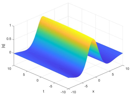
Figure 1. Modulus of the soliton $q(x,t)$ in Equation (85) with the parameters chosen as $\tau =0.5,\zeta =0.2,x_0=0.2,{\sigma }_0=0.2.$

Remark 2.

Because of the difference in Lax pairs, the corresponding R–H problem of the spatial matrix spectral problem is also different. We can clearly see through the solution (85) that the NLS-like equation is different from the single soliton solution of the derivative NLS equation, which also makes the pulse width and velocity of the NLS-like equation corresponding to the derivative NLS equation different.

3.2. Two-Soliton Solutions

When $N=2$, the two-soliton solutions can also be written out explicitly; however, it is quite complicated. For simplicity, we take $N=2$ into Equation (81) and get

$$\begin{array}{cc}\hfill q(x,t)& =-2i\frac{-c_1{e}^{{\theta }_1-{\overline{\theta }}_1}{M}_{22}+c_2{e}^{{\theta }_2-{\overline{\theta }}_1}{M}_{12}}{\left|M\right|}\hfill \\ & \times \frac{c_1{e}^{{\theta }_1-{\overline{\theta }}_2}{M}_{21}-c_2{e}^{{\theta }_2-{\overline{\theta }}_2}{M}_{11}}{\left|M\right|},\hfill \end{array}$$

(86)

where

$$\begin{array}{cc}\hfill M_{11}& =\frac{e^{-({\theta }_1+{\overline{\theta }}_1)}+{\left|c_1\right|}^2{e}^{{\theta }_1+{\overline{\theta }}_1}}{{\overline{\lambda }}_1-{\lambda }_1},\hfill \\ \hfill M_{12}& =\frac{e^{-({\theta }_2+{\overline{\theta }}_1)}+{\overline{c}}_1{c}_2{e}^{{\theta }_2+{\overline{\theta }}_1}}{{\overline{\lambda }}_1-{\lambda }_2},\hfill \\ \hfill M_{21}& =\frac{e^{-({\theta }_1+{\overline{\theta }}_2)}+{\overline{c}}_2{c}_1{e}^{{\theta }_1+{\overline{\theta }}_2}}{{\overline{\lambda }}_2-{\lambda }_1},\hfill \\ \hfill M_{22}& =\frac{e^{-({\theta }_2+{\overline{\theta }}_2)}+{\left|c_2\right|}^2{e}^{{\theta }_2+{\overline{\theta }}_2}}{{\overline{\lambda }}_2-{\lambda }_2}.\hfill \end{array}$$

Then, we show the collision of the two-soliton in Figure 2 and Figure 3. One for the case of ${\zeta }_1\ne {\zeta }_2$ and the other one for the case of ${\zeta }_1={\zeta }_2$. Here,

$${\lambda }_k={\zeta }_k+i{\tau }_k,k=1,2,$$

(87)

where ${\zeta }_k$ is real part of ${\lambda }_k$ and ${\tau }_k$ is imaginary part of ${\lambda }_k$.

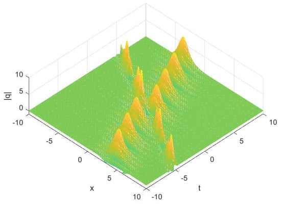
Figure 2. Modulus of the soliton $q(x,t)$ in Equation (86) with the parameters chosen as ${\zeta }_1=1,{\tau }_1=0.75,{\zeta }_2=0.65,{\tau }_2=0.55,c_1=\frac{\sqrt{3}}{2},c_2=-\frac{1}{2}i.$

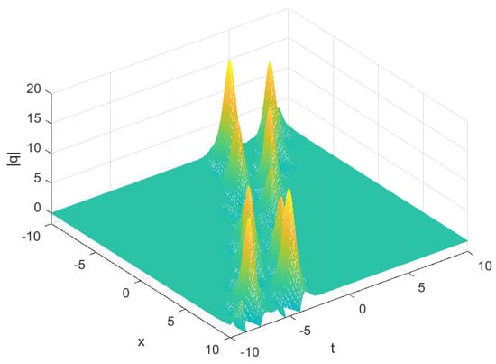
Figure 3. Modulus of the soliton $q(x,t)$ in Equation (86) with the parameters chosen as ${\xi }_1=0.8,{\eta }_1=0.55,{\xi }_2=0.8,{\eta }_2=0.45,c_1=1,c_2=1.$

Case I. We set ${\lambda }_1=1+0.75i,{\lambda }_2=0.65+0.55i.$

In this case, we assume that ${\zeta }_1>{\zeta }_2$, which indicates that soliton-2 is on the left side of soliton-1 as $t\to -\infty$ as well as moves fast. After collision, their position and phase will be scattered. Through asymptotic analysis, we can explain this change.

When $t\to -\infty$, by simple calculation, the asymptotic state of Equation (86) can be expressed as

$$q(x,t)\to 2i({\overline{\lambda }}_1-{\lambda }_1)\frac{c_1^{-}{e}^{{\theta }_1-{\overline{\theta }}_1}}{e^{-({\theta }_1+{\overline{\theta }}_1)}+{\left|c_1^{-}\right|}^2{e}^{{\theta }_1+{\overline{\theta }}_1}},t\to -\infty ,$$

(88)

where $c_1^{-}=c_1\frac{{\lambda }_1-{\lambda }_2}{{\lambda }_1-{\overline{\lambda }}_2}$ and the asymptotic solution has the same peak amplitude $2{\tau }_1$ and velocity $-4({\zeta }_1^2{\tau }_1-{\zeta }_1{\tau }_1^2)$ as Equation (86).

When $t\to +\infty$, the asymptotic state of Equation (86) also can be expressed as

$$q(x,t)\to 2i({\overline{\lambda }}_1-{\lambda }_1)\frac{c_1^{+}{e}^{{\theta }_1-{\overline{\theta }}_1}}{e^{-({\theta }_1+{\overline{\theta }}_1)}+{\left|c_1^{+}\right|}^2{e}^{{\theta }_1+{\overline{\theta }}_1}},t\to +\infty ,$$

(89)

where $c_1^{+}=c_1\frac{{\lambda }_1-{\overline{\lambda }}_2}{{\lambda }_1-{\lambda }_2}.$ The asymptotic solution also has same peak amplitude $2{\tau }_1$ and velocity $-4({\zeta }_1^2{\tau }_1-{\zeta }_1{\tau }_1^2)$ as Equation (86). As Figure 2 shows, the solution does not change their velocity and shape after collision, but the initial positions and phases of solitary waves have shifted.

The position shift is

$$\begin{array}{c}\hfill \Delta x_{01}=-\frac{1}{4{\zeta }_1{\tau }_1}(ln|c_1^{+}|-ln|c_1^{-}\left|\right)=\frac{1}{2{\zeta }_1{\tau }_1}ln\left|\frac{{\lambda }_1-{\lambda }_2}{{\lambda }_1-{\overline{\lambda }}_2}\right|.\end{array}$$

(90)

It is easy to see $\Delta x_{01}<0,$ because ${\lambda }_k\in {\mathbb{C}}_{+}$. Then, the phase shift is

$$\Delta {\sigma }_{01}=arg\left(c_1^{+}\right)-arg\left(c_1^{-}\right)=-2arg\left(\frac{{\lambda }_1-{\lambda }_2}{{\lambda }_1-{\overline{\lambda }}_2}\right).$$

(91)

Similarly, as $t\to \pm \infty ,$ the asymptotic solutions have the same peak amplitude $2{\tau }_2$ and velocity $-4({\zeta }_2^2{\tau }_2-{\zeta }_2{\tau }_2^2)$ with single solitons, where $c_2^{-}=c_1\frac{{\lambda }_2-{\overline{\lambda }}_1}{{\lambda }_2-{\lambda }_1},c_2^{+}=c_1\frac{{\lambda }_2-{\lambda }_1}{{\lambda }_2-{\overline{\lambda }}_1}.$ Therefore, the second soliton position shift is

$$\Delta x_{02}=-\frac{1}{2{\zeta }_2{\tau }_2}ln\left|\frac{{\lambda }_2-{\lambda }_1}{{\lambda }_2-{\overline{\lambda }}_1}\right|>0,$$

(92)

and the phase shift is

$$\Delta {\sigma }_{02}=2arg\left(\frac{{\lambda }_2-{\lambda }_1}{{\lambda }_2-{\overline{\lambda }}_1}\right).$$

(93)

From Equations (90) and (92), we get

$$\frac{\Delta x_{02}}{\Delta x_{01}}=-\frac{{\zeta }_1{\tau }_1}{{\zeta }_2{\tau }_2}.$$

(94)

This shows that the position deviation of each soliton is inversely proportional to its amplitude.

Case II. We set ${\lambda }_1=0.8+0.55i,{\lambda }_2=0.8+0.45i.$

In the second case, we assume that ${\zeta }_1={\zeta }_2$. As Figure 3 shows, the two solitons have the same velocity, and the amplitude function $\left|q\right(x,t\left)\right|$ has periodic oscillations with time.

4. Evolution of the R–H Data in the Perturbed NLS-Like Equation

In this part, a perturbed NLS-like equation

$$i{q}_t+q_{xx}-{2q\left|q\right|}^2+{2a(|q|}^2{)}_{x}q=R^{\prime }\left(q\right)$$

(95)

is analyzed, where Equation (95) is called a nearly integrable system. Here, $R^{\prime }$ is a perturbation term, and $\epsilon \ll 1$. We give the symbol $\frac{\delta }{\delta t}$ to the perturbations in order to distinguish the integrable and perturbation contributions. Consequently,

$$i\frac{\delta Q}{\delta t}=R,R=\left(\begin{array}{cc}0& R^{\prime }\\ -\overline{R^{\prime }}& 0\end{array}\right).$$

Generally, a perturbation leads to a slow evolution of the R–H data. In fact, a perturbation causes the variational $\delta Q$ of the potential of the spectral Equation (15), which leads to the variation of the Jost solutions,

$$\delta J_{\pm x}=-i{\lambda }^2[{\sigma }_3,\delta J_{\pm }]+\delta Q{J}_{\pm }+Q\delta J_{\pm }.$$

By solving the equation, we have

$$\delta J_{\pm }=J_{\pm }E\left({\int }_{\pm \infty }^{x}d{x}^{\prime }{E}^{-1}{J}_{\pm }^{-1}\delta Q{J}_{\pm }E\right)E^{-1}.$$

Hence, by utilizing the Equations (26), (30), and (38), we get a variation of a scattering matrix:

$$\begin{array}{cc}\hfill \frac{\delta S}{\delta t}& =-i\epsilon S_{+}{\int }_{-\infty }^{\infty }dx{E}^{-1}{\left(P^{+}\right)}^{-1}R{P}^{+}E{S}_{-}^{-1}\hfill \\ & =-i\epsilon T_{+}^{-1}{\int }_{-\infty }^{\infty }dx{E}^{-1}{P}^{-}R{\left(P^{-}\right)}^{-1}E{T}_{-}.\hfill \end{array}$$

Here, $S_{\pm }$ and $T_{\pm }$ are the matrices defined in Section 2. Notice that the analytic solution $P^{\pm }$ is naturally installed in the equation. We can thus denote that

$$\begin{array}{c}{\mathrm{Y}}_{+}(a,b)={\int }_a^{b}dx{E}^{-1}{\left(P^{+}\right)}^{-1}R{P}^{+}E,\hfill \\ {\mathrm{Y}}_{-}(a,b)={\int }_a^{b}dx{E}^{-1}{P}^{-}R{\left(P^{-}\right)}^{-1}E,\hfill \\ {\mathrm{Y}}_{\pm }\left(\lambda \right)\equiv {\mathrm{Y}}_{\pm }(-\infty ,\infty ).\hfill \end{array}$$

(96)

Then,

$$\frac{\delta S}{\delta t}=-i\epsilon S_{+}{\mathrm{Y}}_{+}\left(\lambda \right)S_{-}^{-1}=-i\epsilon T_{+}^{-1}{\mathrm{Y}}_{-}\left(\lambda \right)T_{-}.$$

Matrix ${\mathrm{Y}}_{\pm }$ is interrelated through matrix G into the R–H problem (49):

$${\mathrm{Y}}_{-}\left(\lambda \right)=G{\mathrm{Y}}_{+}\left(\lambda \right)G^{-1}.$$

From Equations (30) and (38), the variations of the analytic solutions show

$$\begin{array}{c}\frac{\delta P^{+}}{\delta t}=-i\epsilon P^{+}E{H}_{+}{E}^{-1},\hfill \\ \frac{\delta P^{-}}{\delta t}=i\epsilon E{H}_{-}{E}^{-1}{P}^{-},\hfill \end{array}$$

where $H_{+}$ are the evolution functionals, which are defined as

$$\begin{array}{c}{H}_{+}={\mathrm{Y}}_{+}\left(\lambda \right)H_1-{\mathrm{Y}}_{+}(x,\infty ),\hfill \\ H_{-}=H_1{\mathrm{Y}}_{-}\left(\lambda \right)-{\mathrm{Y}}_{-}(x,\infty ).\hfill \end{array}$$

(97)

From Equation (63), we get the connection between $H_{+}$ and $H_{-}$, $H_{-}=H_{+}^{†},\lambda \in \mathbb{R}\cup i\mathbb{R}$. They contain all the basic information about a perturbation. The additional terms obtained from the perturbation evolution equation $P^{\pm }$ are defined by $H_{\pm }$,

$$\begin{array}{cc}\hfill {\left(P^{+}\right)}_t& =-2i{k}^4[{\sigma }_3,P^{+}]+V{P}^{+}-i\epsilon P^{+}E{H}_{+}{E}^{-1},\hfill \\ \hfill {\left(P^{-}\right)}_t& =-2i{k}^4[{\sigma }_3,P^{-}]-P^{-}V+i\epsilon E{H}_{-}{E}^{-1}{P}^{-}.\hfill \end{array}$$

(98)

In addition, the evolution equation for the matrix G of the R–H problem also has the form

$$G_t=-2i{k}^4[{\sigma }_3,G]-i\epsilon (G{H}_{+}-H_{-}G).$$

(99)

Indeed, the equation provides the evolution of the continuous R–H data.

Next, we derive the perturbation induced evolution equation for the discrete R–H data, i.e., for the zero ${\lambda }_k$ and the eigenvector $v_k$. Vectors $v_{\mathcal{K}}={(v_{\mathcal{K}1},v_{\mathcal{K}2})}^T$ are constant without perturbation. Under perturbation, vectors $v_{\mathcal{K}}={(v_{\mathcal{K}1},v_{\mathcal{K}2})}^T$ have slow t dependence. Let us start with the equation

$$P^{+}\left({\lambda }_k\right)v_k=P^{+}\left({\lambda }_k\right)e^{(-i{\lambda }_k^{2}x-2i\int dt{\lambda }_k^4){\sigma }_3}{v}_{\mathcal{P}}=0$$

which is unaffected by a perturbation. Here, the integral in the exponential takes account of the time dependence of the zero ${\lambda }_k$ caused by the possible perturbation. Taking the total derivative in t, we get

$$\begin{array}{c}\left\{{\left(P^{+}\left(\lambda \right)e^{-i{\lambda }^2{\sigma }_{3}x-2i\int dt{\lambda }_k^4{\sigma }_3}\right)}_t\right.\hfill \\ {\left.+{\left(P^{+}\left(\lambda \right)e^{-i{\lambda }^2{\sigma }_{3}x-2i\int dt{\lambda }_k^4{\sigma }_3}\right)}_{\lambda }{\lambda }_t\right\}}_{\lambda ={\lambda }_k}\hfill \\ +P^{+}\left({\lambda }_k\right)e^{-i{\lambda }_k^2{\sigma }_{3}x-2i\int dt{\lambda }_k^4{\sigma }_3}{\left(v_{\mathcal{P}}\right)}_t=0.\hfill \end{array}$$

The first term with ${\left(P^{+}\right)}_t$ is given by Equation (98), which includes the evolution functional $H_{+}$. Note that the evolution functional $H_{+}\left(\lambda \right)$ is defined by ${\mathrm{Y}}_{+}$ in Equation (97) which depend on ${\left(P^{+}\right)}^{-1}$, conversely. Thus, the function $H_{+}$, which has the simple pole in ${\lambda }_k$, is meromorphic in ${\mathbb{C}}_{+}$, where $P^{+}$ has zero,

$$H_{+}\left(\lambda \right)=H_{+}^{\left(\mathrm{reg}\right)}\left(\lambda \right)+\frac{1}{\lambda -{\lambda }_k}\mathrm{Res}[H_{+}\left(\lambda \right),{\lambda }_k],$$

where $H_{+}^{\left(\mathrm{Res}\right)}$ represents the regular part of $H_{+}$ in the point ${\lambda }_k$. The perturbation evolution of the vector $v_{\mathcal{K}}$ is given by

$${\left(v_{\mathcal{K}}\right)}_t=i\epsilon e^{2i\int dt{\lambda }_k^4{\sigma }_3}{H}_{+}^{\left(\mathrm{reg}\right)}\left({\lambda }_k\right)e^{-2i\int dt{\lambda }_k^4{\sigma }_3}{v}_{\mathcal{K}}.$$

(100)

In order to derive the evolution equation of ${\lambda }_k$, we start with the equation $det{P}^{+}\left({\lambda }_k\right)=0$. Taking the total derivative in t, we get

$${\left[{(det{P}^{+}\left(\lambda \right))}_t\right]}_{\lambda ={\lambda }_k}+{\left[{(det{P}^{+}\left(\lambda \right))}_{\lambda }\right]}_{\lambda ={\lambda }_k}{\left({\lambda }_k\right)}_t=0.$$

From Equations (68) and (70), we have

$$det{P}^{+}\left(\lambda \right)=\frac{\lambda -{\lambda }_k}{\lambda -{\overline{\lambda }}_k}det{\tilde{P}}^{+}\left(\lambda \right),$$

where $det{\tilde{P}}^{+}\left(\lambda \right)\ne 0.$ From Equations (73)–(74), we get

$$v_k=exp\left({\theta }_k{\sigma }_3\right)v_{k0}=\left(\begin{array}{c}exp({\theta }_k+a_k+i{\sigma }_{0k})\\ e^{-{\theta }_k}\end{array}\right).$$

(101)

Here, ${\theta }_k=-i{\lambda }_k^{2}x-2i{\lambda }_k^{4}t,$ and defined $exp(a_k+i{\sigma }_{0k})={\left(v_{k0}\right)}^1/{\left(v_{k0}\right)}^2$, with $a_k$ and ${\sigma }_{0k}$ are real constants. Denote ${[det{P}^{+}\left(\lambda \right)]}_t=i\epsilon \mathrm{tr}{H}_{+}det{P}^{+}\left(\lambda \right)$, we finally get a simple evolution equation for spectral ${\lambda }_k,a_k,{\sigma }_{0k},$

$${\left({\lambda }_k\right)}_t=-i\epsilon \mathrm{Res}[{\mathrm{Y}}_{+22}\left(\lambda \right),{\lambda }_k],$$

(102)

and

$$\begin{array}{c}{(a_k+i{\sigma }_{0k})}_t\hfill \\ ={\mathrm{Y}}_{22}^{\left(\mathrm{reg}\right)}\left({\lambda }_k\right)-exp\left(4i{\int }_0^{t}dt{\lambda }_k^4-a_k-i{\sigma }_{0k}\right){\mathrm{Y}}_{12}^{\left(\mathrm{reg}\right)}\left({\lambda }_k\right).\hfill \end{array}$$

(103)

Perturbation-induced evolution of R–H data is determined by Equations (99), (102), and (103). Notice that these equations are accurate because we have not mentioned any small part of $\epsilon$. In addition, these equations cannot be applied directly, because ${\mathrm{Y}}_{\pm }$ goes in and depends on the unknown solutions $P^{\pm }$ for the spectral problem of the perturbed potential Q.

5. Conclusions

In this paper, an NLS-like equation associated with a $2\times 2$ Lax pair is studied. We start from the spectral analysis of the Lax pair of Equation (2). By using the R–H method, when the scattering coefficients vanish, the regularization condition at the infinity on the real axis can be used to solve the corresponding R–H problem. When the jump matrix G is the unit matrix, the N-soliton solutions of the integrable equation can be obtained. The R–H method is a very useful tool, especially for soliton solutions. As we all know, the R–H approach has been widely used to solve many integrable equations, for example, the generalized Sasa–Satsuma equation [14], the general coupled nonlinear Schrödinger equation [49], and the Harry–Dym equation [50]. Furthermore, based on the R–H problem, the evolution functional is derived and the R–H data in the perturbed NLS-like equation is obtained. Perturbation theory has many applications, such as propagation of arbitrarily polarized optical pulses in optical fibers, multicomponent soliton equations, and soliton pulses in various Bose–Einstein condensations.

It is very meaningful to study the exact solutions and other types of integrable equations, and to analyze perturbation theory based on R–H problems. Further research on how to apply the R–H problem to the generalized integrable correspondence equation combined with perturbation theory will be one of our future considerations.

References

- Ablowitz, M.J.; Kaup, D.J.; Newell, A.C.; Segur, H. The inverse scattering Transform-Fourier analysis for nonlinear problems. Stud. Appl. Math. 2015, 53, 249–315. [Google Scholar] [CrossRef]
- Ji, J.L.; Zhu, Z.N. Soliton solutions of an integrable nonlocal modified Korteweg-de Vries equation through inverse scattering transform. J. Math. Anal. Appl. 2017, 453, 973–984. [Google Scholar] [CrossRef]
- Maeda, M.; Sasaki, H.; Segawa, E.; Suzuki, A.; Suzuki, K. Scattering and inverse scattering for nonlinear quantum walks. Discrete Contin. Dyn. Syst. 2018, 38, 18. [Google Scholar] [CrossRef]
- Shchesnovich, V.S. The soliton perturbation theory based on the Riemann-Hilbert spectral problem. Chaos Solitons Fractals 1995, 5, 2121–2133. [Google Scholar] [CrossRef]
- Kaup, D.J.; Yang, J.K. The inverse scattering transform and squared eigenfunctions for a degenerate 3 × 3 operator. Inverse Probl. 2009, 25, 105010–105021. [Google Scholar] [CrossRef]
- Guo, B.L.; Ling, L.M. Riemann-Hilbert approach and N-soliton formula for coupled derivative Schrödinger equation. J. Math. Phys. 2012, 53, 73506. [Google Scholar] [CrossRef]
- Wang, D.S.; Ma, Y.Q.; Li, X.G. Prolongation structures and matter-wave solitons in F = 1 spinor Bose-Einstein condensate with time-dependent atomic scattering lengths in an expulsive harmonic potential. Commun. Nonlinear Sci. Numer. Simul. 2014, 19, 3556–3569. [Google Scholar] [CrossRef]
- Huang, L.; Lenells, J. Nonlinear Fourier transforms for the sine-Gordon equation in the quarter plane. J. Differ. Equ. 2017, 264, 3445–3499. [Google Scholar] [CrossRef]
- Zakharov, V.E.; Shabat, A.B. Integration of nonlinear equations of mathematical physics by the method of inverse scattering. II. Funct. Anal. Appl. 1979, 13, 166–174. [Google Scholar] [CrossRef]
- Novikov, S.; Manakov, S.V.; Pitaevskii, L.P.; Zakharov, V.E. Theory of Solitons: The Inverse Scattering Method; Springer Science and Business Media: New York, NY, USA, 1984. [Google Scholar]
- Deift, P.; Zhou, X. A steepest descent method for oscillatory Riemann-Hilbert problems. Bull. Aust. Math. Soc. 1991, 26, 295–368. [Google Scholar] [CrossRef]
- Shchesnovich, V.S.; Yang, J.K. General soliton matrices in the Riemann-Hilbert problem for integrable nonlinear equations. J. Math. Phys. 2003, 44, 4604–4639. [Google Scholar] [CrossRef]
- Webb, J.R.L.; Infante, G. Positive solutions of nonlocal boundary value problems: A unified approach. J. Lond. Math. Soc. 2006, 74, 673–693. [Google Scholar] [CrossRef]
- Geng, X.G.; Wu, J.P. Riemann-Hilbert approach and N-soliton solutions for a generalized Sasa-Satsuma equation. Wave Motion 2016, 60, 62–72. [Google Scholar] [CrossRef]
- Ma, W.X. Riemann-Hilbert problems and N-soliton solutions for a coupled mKdV system. J. Geom. Phys. 2018, 132, 45–54. [Google Scholar] [CrossRef]
- Xu, X.X.; Sun, Y.P. An integrable coupling hierarchy of Dirac integrable hierarchy, its Liouville integrability and Darboux transformation. J. Nonlinear Sci. Appl. 2017, 10, 3328–3343. [Google Scholar] [CrossRef]
- Chen, J.C.; Ma, Z.Y.; Hu, Y.H. Nonlocal symmetry, Darboux transformation and soliton-cnoidal wave interaction solution for the shallow water wave equation. J. Math. Anal. Appl. 2018, 460, 987–1003. [Google Scholar] [CrossRef]
- Zhang, N.; Xia, T.C.; Jin, Q.Y. N-Fold Darboux transformation of the discrete Ragnisco-Tu system. Adv. Differ. Equ. 2018, 2018, 302. [Google Scholar] [CrossRef]
- Zhu, S.D.; Song, J.F. Residual symmetries, nth Bäcklund transformation and interaction solutions for (2+1)-dimensional generalized Broer-Kaup equations. Appl. Math. Lett. 2018, 83, 33–39. [Google Scholar] [CrossRef]
- Chen, H.H. General derivation of Bäcklund transformations from inverse scattering problems. Phys. Rev. Lett. 1974, 33, 925–928. [Google Scholar] [CrossRef]
- Wazwaz, A.M. Multiple-soliton solutions for the KP equation by Hirota’s bilinear method and by the tanh-coth method. Appl. Math. Comput. 2007, 190, 633–640. [Google Scholar] [CrossRef]
- Hu, X.B.; Wu, Y.T. Application of the Hirota bilinear formalism to a new integrable differential-difference equation. Phys. Lett. A 1998, 246, 523–529. [Google Scholar] [CrossRef]
- Ma, W.X.; Zhou, Y. Lump solutions to nonlinear partial differential equations via Hirota bilinear forms. J. Differ. Equ. 2018, 264, 2633–2659. [Google Scholar] [CrossRef]
- Fan, E.G.; Zhang, H.Q. The homogeneous balance method for solving nonlinear soliton equations. Acta Phys. Sin. 1998, 47, 353–362. [Google Scholar]
- Wang, M.L.; Zhou, Y.B.; Li, Z.B. Application of a homogeneous balance method to exact solutions of nonlinear equations in mathematical physics. Phys. Lett. A 1996, 216, 67–75. [Google Scholar] [CrossRef]
- Ma, W.X.; Wu, H.Y.; He, J.S. Partial differential equations possessing Frobenius integrable decompositions. Phys. Lett. A 2007, 364, 29–31. [Google Scholar] [CrossRef]
- Gao, L.; Ma, W.X.; Xu, W. Frobenius integrable decompositions for ninth-order partial differential equations of specific polynomial type. Appl. Math. Comput. 2010, 216, 2728–2733. [Google Scholar] [CrossRef]
- Fang, Y.; Dong, H.H.; Hou, Y.J.; Kong, Y. Frobenius integrable decompositions Of nonlinear evolution equations with modified term. Appl. Math. Comput. 2014, 226, 435–440. [Google Scholar] [CrossRef]
- Xu, T.; Tian, B. An extension of the Wronskian technique for the multicomponent Wronskian solution to the vector nonlinear Schrödinger equation. J. Math. Phys. 2010, 51, 359. [Google Scholar] [CrossRef]
- Corona-Corona, G. A Wronskian of Jost solutions. J. Math. Phys. 2004, 45, 4282–4287. [Google Scholar] [CrossRef]
- Yang, J.Y.; Ma, W.X.; Qin, Z.Y. Lump and lump-soliton solutions to the (2+1)-dimensional Ito equation. Anal. Math. Phys. 2018, 8, 427–436. [Google Scholar] [CrossRef]
- Zhang, Y.; Dong, H.; Zhang, X.; Yang, H. Rational solutions and lump solutions to the generalized (3+1)-dimensional Shallow Water-like equation. Comput. Math. Appl. 2017, 73, 246–252. [Google Scholar] [CrossRef]
- Yong, X.L.; Ma, W.X.; Huang, Y.H.; Liu, Y. Lump solutions to the Kadomtsev-Petviashvili I equation with a self-consistent source. Comput. Math. Appl. 2018, 75, 2633–2659. [Google Scholar] [CrossRef]
- Wang, H. Lump and interaction solutions to the (2+1)-dimensional Burgers equation. Appl. Math. Lett. 2018, 85, 27–34. [Google Scholar] [CrossRef]
- Zeng, Z.J. Periodic solutions of a discrete time non-autonomous ratio-dependent predator-prey system with control. Commun. Korean Math. Soc. 2007, 22, 465–474. [Google Scholar] [CrossRef]
- Rostworowski, A. Higher order perturbations of Anti-de Sitter space and time-periodic solutions of vacuum Einstein equations. Phys. Rev. D 2017, 95, 16. [Google Scholar] [CrossRef]
- Savulescu, J. Wicked problems, complex solutions, and the cost of trust. J. Med. Ethics 2018, 44, 147–148. [Google Scholar] [CrossRef] [PubMed][Green Version]
- Datsko, B.; Gafiychuk, V. Complex spatio-temporal solutions in fractional reaction-diffusion systems near a bifurcation point. Fract. Calc. Appl. Anal. 2018, 21, 237–253. [Google Scholar] [CrossRef]
- Zhu, Q.Z.; Xu, J.; Fan, E.G. The Riemann-Hilbert problem and long-time asymptotics for the Kundu-Eckhaus equation with decaying initial value. Appl. Math. Lett. 2017, 76, 81–89. [Google Scholar] [CrossRef]
- Tian, S.F. Initial-boundary value problems for the general coupled nonlinear Schrödinger equation on the interval via the Fokas method. J. Differ. Equ. 2017, 262, 506–558. [Google Scholar] [CrossRef]
- Zhang, N.; Xia, T.C.; Fan, E.G. A Riemann-Hilbert Approach to the Chen-Lee-Liu Equation on the Half Line. Acta. Math. Appl. Engl. Ser. 2018, 34, 493–515. [Google Scholar] [CrossRef]
- Song, G.H.; Shin, S.Y. Design of corrugated waveguide filters by the Gel’fand-Levitan-Marchenko inverse-scattering method. J. Opt. Soc. Am. A 1985, 2, 1905–1915. [Google Scholar] [CrossRef]
- Kivshar, Y.S.; Zhang, F.; Takeno, S. Multistable nonlinear surface modes. Phys. D 1998, 119, 125–133. [Google Scholar] [CrossRef]
- McLaughlin, D.W.; Scott, A.C. Perturbation analysis of fluxon dynamics. Phys. Rev. A 1978, 18, 1652. [Google Scholar] [CrossRef]
- Kivshar, Y.S.; Malomed, B.A. Dynamics of solitons in nearly integrable systems. Rev. Mod. Phys. 1989, 61, 763. [Google Scholar] [CrossRef]
- Shchesnovich, V.S. Perturbation theory for nearly integrable multicomponent nonlinear PDEs. J. Math. Phys. 2002, 43, 1460–1486. [Google Scholar] [CrossRef][Green Version]
- Doktorov, E.V.; Wang, J.D.; Yang, J.K. Perturbation theory for bright spinor Bose-Einstein condensate solitons. Phys. Rev. A 2008, 77, 043617. [Google Scholar] [CrossRef]
- Kaup, D.J. Integrable systems and squared eigenfunctions. Theor. Math. Phys. 2009, 159, 806–818. [Google Scholar] [CrossRef]
- Wang, D.S.; Zhang, D.J.; Yang, J.K. Integrable properties of the general coupled nonlinear Schrödinger equations. J. Math. Phys. 2010, 51, 133–148. [Google Scholar] [CrossRef]
- Xiao, Y.; Fan, E.G. A Riemann-Hilbert approach to the Harry-Dym equation on the Line. Chin. Ann. Math. Ser. B 2014, 37, 373–384. [Google Scholar] [CrossRef]
© 2019 by the authors. Licensee MDPI, Basel, Switzerland. This article is an open access article distributed under the terms and conditions of the Creative Commons Attribution (CC BY) license (http://creativecommons.org/licenses/by/4.0/).