Article

Inference about the Ratio of the Coefficients of Variation of Two Independent Symmetric or Asymmetric Populations

1
Teaching and Research Section of Public Education, Hainan Radio and TV University, No.20 Haidianerxi Road, Meilan District, Haikou 570208, Hainan, China
2
Department of Mathematics, Faculty of Art and Sciences, Cankaya University, 0630 Ankara, Turkey
3
Institute of Space Sciences, 077125 Magurele-Bucharest, Romania
*
Author to whom correspondence should be addressed.
Symmetry 2019, 11(6), 824; https://doi.org/10.3390/sym11060824
Submission received: 23 May 2019 / Revised: 13 June 2019 / Accepted: 20 June 2019 / Published: 21 June 2019
(This article belongs to the Special Issue Symmetry in Applied Continuous Mechanics)

Abstract

:
Coefficient of variation (CV) is a simple but useful statistical tool to make comparisons about the independent populations in many research areas. In this study, firstly, we proposed the asymptotic distribution for the ratio of the CVs of two separate symmetric or asymmetric populations. Then, we derived the asymptotic confidence interval and test statistic for hypothesis testing about the ratio of the CVs of these populations. Finally, the performance of the introduced approach was studied through simulation study.

1. Introduction

Based on the literature, to describe a dataset (random variable), three main characteristics containing central tendencies, dispersion tendencies and shape tendencies, are used. A central tendency (or measure of central tendency) is a central or typical value for a random variable that describes the way in which the random variable is clustered around a central value. It may also be called a center or location of the distribution of the random variable. The most common measures of central tendency are the mean, the median and the mode. Measures of dispersion like the range, variance and standard deviation tell us about the spread of the values of a random variable. It may also be called a scale of the distribution of the random variable. The shape tendencies such as skewness and kurtosis describe the distribution (or pattern) of the random variable.
The division of the standard deviation to the mean of population, C V = σ μ , is called as coefficient of variation (CV) which is an applicable statistic to evaluate the relative variability. This free dimension parameter can be widely used as an index of reliability or variability in many applied sciences such as agriculture, biology, engineering, finance, medicine, and many others [1,2,3]. Since it is often necessary to relate the standard deviation to the level of the measurements, the CV is a widely used measure of dispersion. The CVs are often calculated on samples from several independent populations, and questions about how to compare them naturally arise, especially when the distributions of the populations are skewed. In real world applications, the researchers may intend to compare the CVs of two separate populations to understand the structure of the data. ANOVA and Levene tests can be used to investigate the equality of CVs of populations in case the means or variances of the populations are equal. It is obvious that in many situations two populations with different means and variances may have an equal CV. For the normal case, the problems of interval estimating the CV or comparison of two or several CVs have been well addressed in the literature. Due to possible small differences of two small CVs and no strong interpretation, the ratio of CVs is more accurate than the difference of CVs. Bennett [4] proposed a likelihood ratio test. Doornbos and Dijkstra [5] and Hedges and Olkin [6] presented two tests based on the non-central t test. A modification of Bennett’s method was provided by Shafer and Sullivan [7]. Wald tests have been introduced by [8,9,10]. Based on Renyi’s divergence, Pardo and Pardo [11] proposed a new method. Nairy and Rao [12] applied the likelihood ratio, score test and Wald test to check that the inverse CVs are equal. Verrill and Johnson [13] applied one-step Newton estimators to establish a likelihood ratio test. Jafari and Kazemi [14] developed a parametric bootstrap (PB) approach. Some statisticians improved these tests for symmetric distributions [15,16,17,18,19,20,21,22,23]. The problem of comparing two or more CVs arises in many practical situations [24,25,26]. Nam and Kwon [25] developed approximate interval estimation of the ratio of two CVs for lognormal distributions by using the Wald-type, Fieller-type, log methods, and the method of variance estimates recovery (MOVER). Wong and Jiang [26] proposed a simulated Bartlett corrected likelihood ratio approach to obtain inference concerning the ratio of two CVs for lognormal distribution.
In applications, it is usually assumed that the data follows symmetric distributions. For this reason, most previous works have focused on the comparison of CVs in symmetric distributions, especially normal distributions. In this paper, we propose a method to compare the CVs of two separate symmetric or asymmetric populations. Firstly, we propose the asymptotic distribution for the ratio of the CVs. Then, we derive the asymptotic confidence interval and test statistic for hypothesis testing about the ratio of the CVs. Finally, the performance of the introduced approach is studied through simulation study. The introduced approach seems to have many advantages. First, it is powerful. Second, it is not too computational. Third, it can be applied to compare the CVs of two separate symmetric or asymmetric populations. We apply a methodology similar to that which has been used in [27,28,29,30,31,32,33]. The comparison between the parameters of two datasets or models has been considered in several works [34,35,36,37,38,39,40]

2. Asymptotic Results

Assume that X and Y are uncorrelated variables with non-zero means μ X and μ Y , and the finite i t h central moments:
μ i X = E ( X μ X ) i ,      μ i Y = E ( Y μ Y ) i ,      i { 2 , 3 , 4 } ,
respectively. Also assume two samples X 1 , , X m , and Y 1 , , Y n , distributed from X and Y , respectively. From the motivation given in the introduction, the parameter:
γ = C V Y C V X ,
is interesting to inference, where C V Y and C V X are the CVs corresponding to Y and X , respectively.
Assume m i X = 1 m k = 1 m ( x k x ¯ ) i    , m i Y = 1 n k = 1 n ( y k y ¯ ) i ,    i { 2 , 3 , 4 } . C V X and C V Y , are consistently estimated [41] by C ^ V X = m 2 X X ¯ and C ^ V Y = m 2 Y Y ¯ , respectively. So, it is obvious that
γ ^ = C ^ V Y C ^ V X
can reasonably estimate the parameter γ . For simplicity, let m = n . When n = m , let n * = m i n ( m , n ) instead of m and n in the following discussions.
Lemma 1.
If the above assumptions are satisfied, then:
n ( C ^ V X C V X ) L N ( 0 , δ X 2 ) ,      a s      n ,
where:
δ X 2 = [ μ 4 X μ 2 X 2 4 μ X 2 μ 2 X μ 3 X μ X 3 + μ 2 X 2 μ 4 X ] ,
is the asymptotic variance.
Proof. 
The outline of proof can be found in [41]. □
The next theorem corresponds to the asymptotic distribution of γ ^ . This theorem will be applied to construct the confidence interval and perform hypothesis testing for the parameter γ .
Theorem 1.
If the previous assumptions are satisfied, then:
n ( γ ^ γ ) L N ( 0 , λ 2 ) ,      a s    n ,
where:
λ 2 = 1 C V X 2 ( γ 2 δ X 2 + δ Y 2 ) ,
and:
δ Y 2 = [ μ 4 Y μ 2 Y 2 4 μ Y 2 μ 2 Y μ 3 Y μ Y 3 + μ 2 Y 2 μ 4 Y ] .
Proof. 
By using Lemma 1, we have:
n ( C ^ V X C V X ) L N ( 0 , δ X 2 ) ,      a s    n ,
and:
n ( C ^ V Y C V Y ) L N ( 0 , δ Y 2 ) ,      a s    n .
Slutsky’s Theorem gives:
n [ ( C ^ V X C ^ V Y ) ( C V X C V Y ) ] L N ( 0 , ( δ X 2 0 0 δ Y 2 ) ) ,
for independent samples [41].
Now define f :    R 2 R as f ( x , y ) = y x . Then we have:
f ( x , y ) = ( y x 2 , 1 x ) ,
where f ( x , y ) is the gradient function. Consequently, we have f ( C V X , C V Y ) ( f ( C V X , C V Y ) ) T = λ 2 . Because of continuity of f in the neighbourhood of ( C V X , C V Y ) , by using Cramer’s Rule:
n ( f ( C ^ V X , C ^ V Y ) f ( C V X , C V Y ) ) = n ( γ ^ γ ) L N ( 0 , λ 2 ) ,    n ,
the proof ends. □
Thus, the asymptotic distribution can be constructed as:
T n = n ( γ ^ γ λ ) L N ( 0 , 1 ) ,      a s    n .

2.1. Constructing the Confidence Interval

As can be seen, the parameter λ depends on C V X , δ X 2 , δ Y 2 and γ which are unknown parameters in practice. The result of the next theorem can be applied to construct the confidence interval and to perform the hypothesis testing for the parameter γ .
Theorem 2.2:
If the previous assumptions are satisfied, then:
T n * = n ( γ ^ γ λ ^ ) L N ( 0 , 1 ) ,      a s ,
where:
λ ^ 2 = 1 C ^ V X 2 ( γ ^ 2 δ ^ X 2 + δ ^ Y 2 ) ,
δ ^ X 2 = [ m 4 X m 2 X 2 4 X ¯ 2 m 2 X m 3 X X ¯ 3 + m 2 X 2 m 4 X ] ,
and:
δ ^ Y 2 = [ m 4 Y m 2 Y 2 4 Y ¯ 2 m 2 Y m 3 Y Y ¯ 3 + m 2 Y 2 m 4 Y ] .
Proof. 
From the Weak Law of Large Numbers, it is known that:
X ¯ p μ X ,      Y ¯ p μ Y ,    m i X p μ i X ,      m i Y p μ i Y ,      i { 2 , 3 , 4 } ,
as n .
Consequently, by applying Slutsky’s Theorem, we have λ ^ p λ , as n . Appliying Theorem 1 the proof is completed. □
Now, T n * is a pivotal quantity for γ . In the following, this pivotal quantity is used to construct asymptotic confidence interval for γ .
( γ ^ λ ^ n Z α 2 , γ ^ + λ ^ n Z α 2 ) .

2.2. Hypothesis Testing

In real word applications, researchers are interested in testing about the parameter γ . For example, the null hypothesis H 0 : γ = 1 means that the CVs of two populations are equal. To perform the hypothesis test H 0 :    γ = γ 0 , the test statistic:
T 0 = n ( γ ^ γ 0 λ * ) ,
is generally applied, such that:
λ * 2 = 1 C ^ V X 2 ( γ 0 2 δ ^ X 2 + δ ^ Y 2 ) .
If the null hypothesis H 0 : γ = γ 0 is satisfied, then the asymptotic distribution of T 0 is standard normal.

2.3. Normal Populations

Naturally, many phenomena follow normal distribution. This distribution is very important in natural and social sciences. Many researchers focused on the comparison between the CVs of two independent normal distributions. Nairy and Rao [12] reviewed and studied several methods such as likelihood ratio test, score test and Wald test that could be used to compare the CVs of two independent normal distributions. If the parent distributions X and Y are normal, then:
μ 3 X = μ 3 Y = 0 ,        μ 4 X = 3 μ 2 X 2 ,    μ 4 Y = 3 μ 2 Y 2 .
Consequently, for normal distributions, δ X 2 and δ ^ X 2 can be rewritten as:
δ X 2 = μ 2 X μ X 2 + 2 μ 2 X 2 2 μ X 4 ,
and:
δ ^ X 2 = m 2 X X ¯ 2 + 2 m 2 X 2 2 X ¯ 4 ,
respectively.

3. Simulation Study

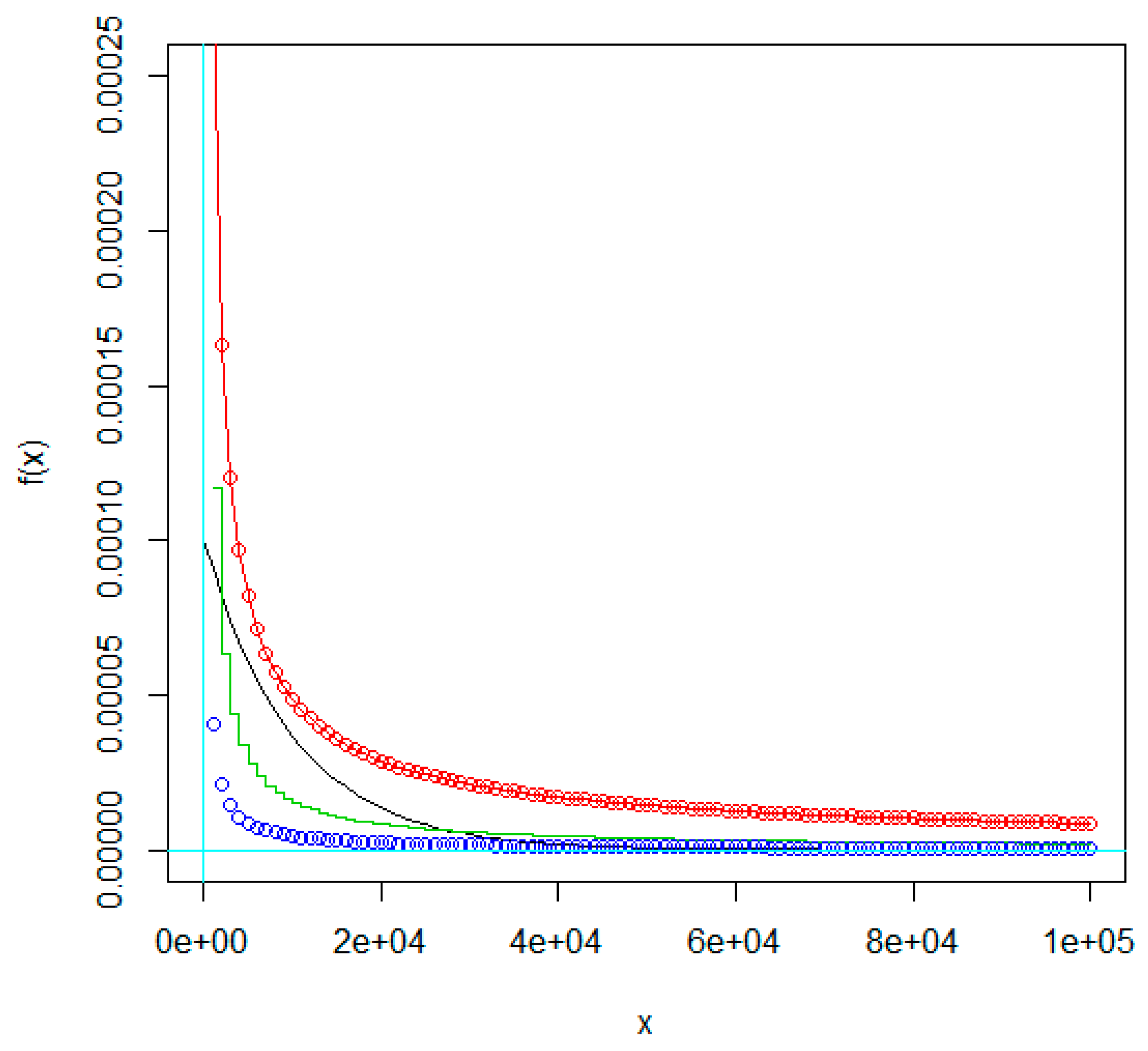
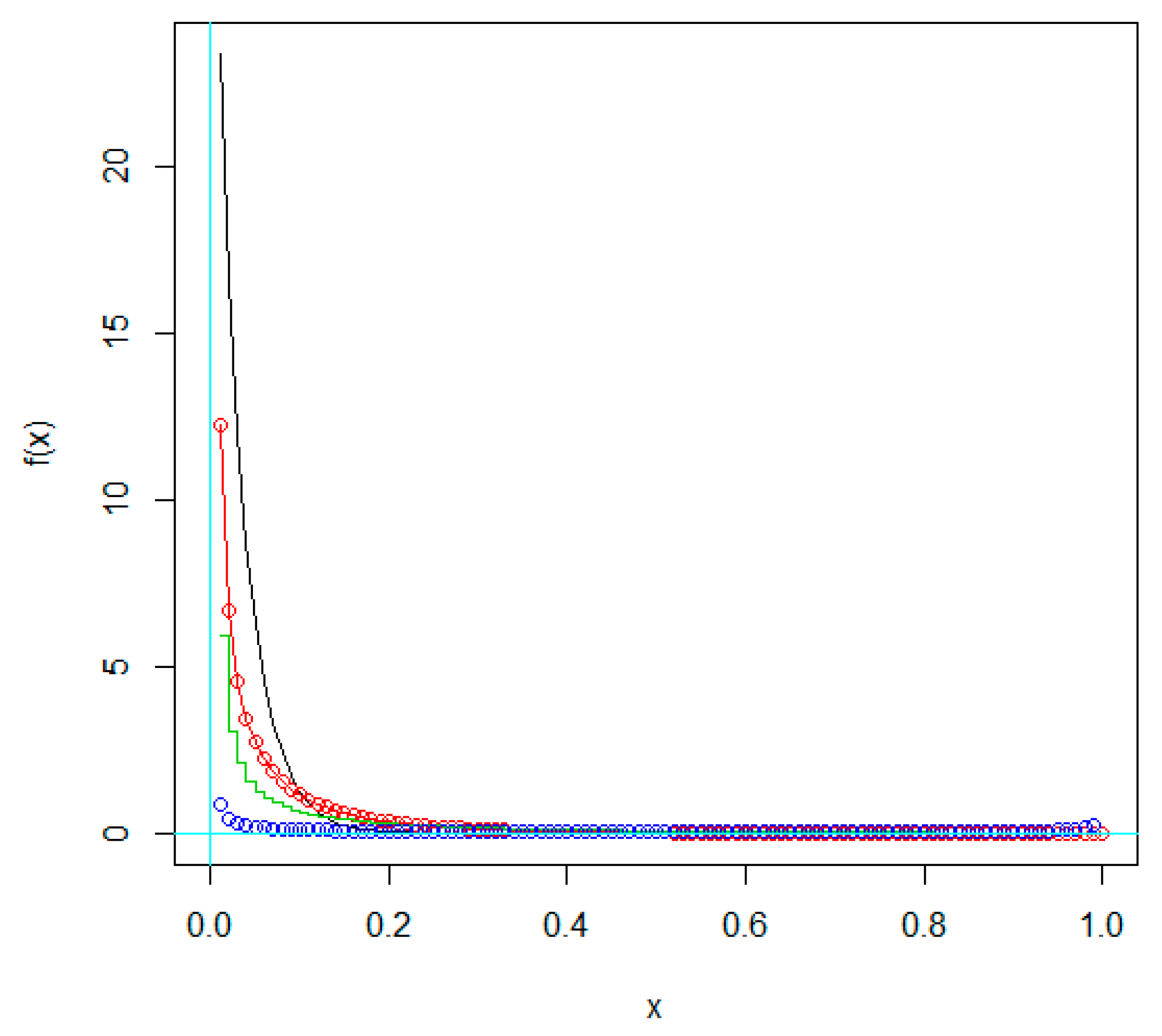
In this section, the accuracy of the given theoretical results is studied and analyzed by different simulated datasets. For the populations X and Y , we respectively simulated different samples from symmetric distribution (normal) and asymmetric distributions (gamma and beta) with different CV values, ( C V X , C V Y ) { ( 1 , 1 ) , ( 1 , 2 ) , ( 2 , 3 ) , ( 2 , 5 ) } , which are equivalent to γ { 1 , 2 , 1.5 , 2.5 } . Figure 1, Figure 2 and Figure 3 show the plots of probability density function (PDF) for the considered distributions.
The simulations are accomplished after 1000 runs using the R 3.3.2 software (R Development Core Team, 2017) on a PC (Processor: Intel(R) CoreTM(2) Duo CPU T7100 @ 1.80GHz 1.80GHz, RAM: 2.00GB, System Type: 32-bit).
To check the accuracy of Equations (3) and (4), we estimated the coverage probability,
CP   =   number   of   runs   that   Equation   (   3   )   contained   true   γ 1000 ,
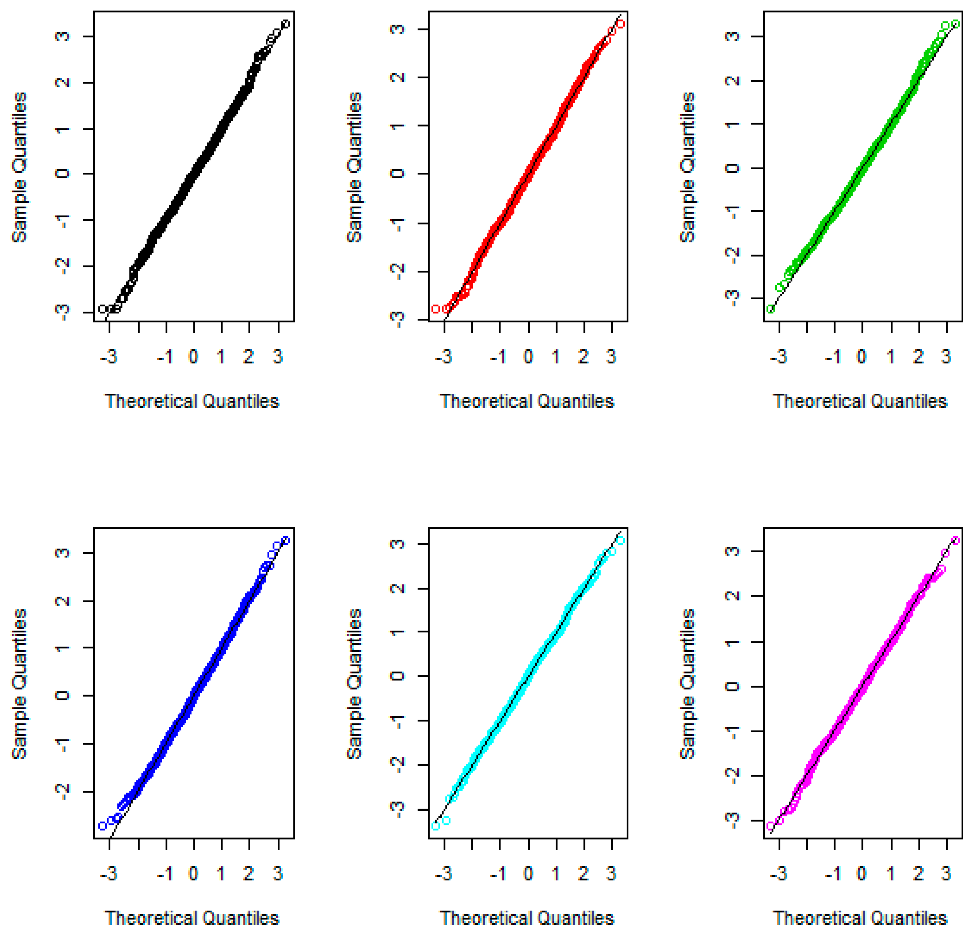
for each parameter setting. We also computed the value of the test statistic in Equation (4), for each run. Then we considered the Shapiro–Wilk’s normality test and the Q–Q plots to verify normality assumption for the proposed test statistic. Table 1 summarizes the CP values for different parameter settings.
As Table 1 indicates, the CP are very close to the considered level ( 1 α = 0.95 ), especially when sample size was increased, and consequently the proposed method controlled the type I error. In other words, about 95 % of simulated confidence intervals contained true γ and consequently it can be accepted that Equation (3) is asymptotically confidence interval for γ . The values of CPU times (in seconds) for different parameter settings given in Table 2, verify that this approach is not too time consuming. Furthermore, Figure 4 and Table 3 illustrate the Q-Q plots and the p-values of Shapiro–Wilk’s test, respectively, to study the normality of the introduced test statistic.
First column:
Up :   ( C V X , C V Y ) = ( 1 , 1 )   and    ( m , n ) = ( 50 , 100 ) ;   down :   ( C V X , C V Y ) = ( 1 , 2 )   and   ( m , n ) = ( 75 , 100 ) .
Second column:
Up :   ( C V X , C V Y ) = ( 1 , 2 )   and    ( m , n ) = ( 100 , 200 ) ;   down :   ( C V X , C V Y ) = ( 2 , 3 )   and    ( m , n ) = ( 200 , 300 ) .
Third column:
Up :   ( C V X , C V Y ) = ( 2 , 3 )   and    ( m , n ) = ( 500 , 700 ) ;   down :   ( C V X , C V Y ) = ( 3 , 5 )   and    ( m , n ) = ( 700 , 1000 ) .
Table 3 indicates that all p-values are more than 0.05 and consequently the Shapiro–Wilk’s test verified the normality of the proposed test statistic. This result could also be derived from Q-Q plots. Since the points form almost a straight line, the observed quantiles are very similar to the quantiles of theoretical distribution (normal). Therefore, the simulation results verify that the asymptotic theoretical results seem to be quite satisfying for all parameter settings. Consequently our proposed approach is a good choice to perform hypothesis testing and to establish a confidence interval for the ratio of the CVs in two separate populations.

4. Conclusions

Coefficient of variation is a simple but useful statistical tool to make comparisons about independent populations. In many situations two populations with different means and variances may have equal CVs. In real world applications, researchers may intend to study the similarity of the CVs in two separate populations to understand the structure of the data. Due to possible small differences of two small CVs and no strong interpretation, the ratio of CVs is more accurate than the difference of the CVs. In this study, we proposed the asymptotic distribution, derived the asymptotic confidence interval and established hypothesis testing for the ratio of the CVs in two separate populations. The results indicated that the coverage probabilities are very close to the considered level, especially when sample sizes were increased, and consequently the proposed method controlled the type I error. The values of CPU times also verified that this approach is not too time consuming. Shapiro–Wilk’s normality test and Q-Q plots also verified the normality of the proposed test statistic. The results verified that the asymptotic approximations were satisfied for all simulated datasets and the introduced technique acted well in constructing CI and performing tests of hypothesis.

Author Contributions

Conceptualization, Z.Y. and D.B.; formal analysis, Z.Y. and D.B. investigation, Z.Y. and D.B.; methodology, Z.Y. and D.B.; resources, Z.Y. and D.B.; software, Z.Y. and D.B.; supervision, Z.Y. and D.B.; visualization, Z.Y. and D.B.; writing—original draft, Z.Y. and D.B.; writing—review & editing, D.B.

Funding

This research received no external funding.

Conflicts of Interest

The authors declare no conflict of interest.

References

  1. Meng, Q.; Yan, L.; Chen, Y.; Zhang, Q. Generation of Numerical Models of Anisotropic Columnar Jointed Rock Mass Using Modified Centroidal Voronoi Diagrams. Symmetry 2018, 10, 618. [Google Scholar] [CrossRef]
  2. Aslam, M.; Aldosari, M.S. Inspection Strategy under Indeterminacy Based on Neutrosophic Coefficient of Variation. Symmetry 2019, 11, 193. [Google Scholar] [CrossRef]
  3. Iglesias-Caamaño, M.; Carballo-López, J.; Álvarez-Yates, T.; Cuba-Dorado, A.; García-García, O. Intrasession Reliability of the Tests to Determine Lateral Asymmetry and Performance in Volleyball Players. Symmetry 2018, 10, 16. [Google Scholar] [CrossRef]
  4. Bennett, B.M. On an approximate test for homogeneity of coefficients of variation. In Contribution to Applied Statistics; Ziegler, W.J., Ed.; Birkhauser Verlag: Basel, Switzerland; Stuttgart, Germany, 1976; pp. 169–171. [Google Scholar]
  5. Doornbos, R.; Dijkstra, J.B. A multi sample test for the equality of coefficients of variation in normal populations. Commun. Stat. Simul. Comput. 1983, 12, 147–158. [Google Scholar] [CrossRef]
  6. Hedges, L.; Olkin, I. Statistical Methods for Meta-Analysis; Academic Press: Orlando, FL, USA, 1985. [Google Scholar]
  7. Shafer, N.J.; Sullivan, J.A. A simulation study of a test for the equality of the coefficients of variation. Commun. Stat. Simul. Comput. 1986, 15, 681–695. [Google Scholar] [CrossRef]
  8. Rao, K.A.; Vidya, R. On the performance of test for coefficient of variation. Calcutta Stat. Assoc. Bull. 1992, 42, 87–95. [Google Scholar] [CrossRef]
  9. Gupta, R.C.; Ma, S. Testing the equality of coefficients of variation in k normal populations. Commun. Stat. Theory Methods 1996, 25, 115–132. [Google Scholar] [CrossRef]
  10. Rao, K.A.; Jose, C.T. Test for equality of coefficient of variation of k populations. In Proceedings of the 53rd Session of International Statistical Institute, Seoul, Korea, 22–29 August 2001. [Google Scholar]
  11. Pardo, M.C.; Pardo, J.A. Use of Rényi’s divergence to test for the equality of the coefficient of variation. J. Comput. Appl. Math. 2000, 116, 93–104. [Google Scholar] [CrossRef]
  12. Nairy, K.S.; Rao, K.A. Tests of coefficient of variation of normal population. Commun. Stat. Simul. Comput. 2003, 32, 641–661. [Google Scholar] [CrossRef]
  13. Verrill, S.; Johnson, R.A. Confidence bounds and hypothesis tests for normal distribution coefficients of variation. Commun. Stat. Theory Methods 2007, 36, 2187–2206. [Google Scholar] [CrossRef]
  14. Jafari, A.A.; Kazemi, M.R. A parametric bootstrap approach for the equality of coefficients of variation. Comput. Stat. 2013, 28, 2621–2639. [Google Scholar] [CrossRef]
  15. Feltz, G.J.; Miller, G.E. An asymptotic test for the equality of coefficients of variation from k normal populations. Stat. Med. 1996, 15, 647–658. [Google Scholar] [CrossRef]
  16. Fung, W.K.; Tsang, T.S. A simulation study comparing tests for the equality of coefficientsof variation. Stat. Med. 1998, 17, 2003–2014. [Google Scholar] [CrossRef]
  17. Tian, L. Inferences on the common coefficient of variation. Stat. Med. 2005, 24, 2213–2220. [Google Scholar] [CrossRef] [PubMed]
  18. Forkman, J. Estimator and Tests for Common Coefficients of Variation in Normal Distributions. Commun. Stat. Theory Methods 2009, 38, 233–251. [Google Scholar] [CrossRef] [Green Version]
  19. Liu, X.; Xu, X.; Zhao, J. A new generalized p-value approach for testing equality of coefficients of variation in k normal populations. J. Stat. Comput. Simul. 2011, 81, 1121–1130. [Google Scholar] [CrossRef]
  20. Krishnamoorthy, K.; Lee, M. Improved tests for the equality of normal coefficients of variation. Comput. Stat. 2013, 29, 215–232. [Google Scholar] [CrossRef]
  21. Jafari, A.A. Inferences on the coefficients of variation in a multivariate normal population. Commun. Stat. Theory Methods 2015, 44, 2630–2643. [Google Scholar] [CrossRef]
  22. Hasan, M.S.; Krishnamoorthy, K. Improved confidence intervals for the ratio of coefficients of variation of two lognormal distributions. J. Stat. Theory Appl. 2017, 16, 345–353. [Google Scholar] [CrossRef]
  23. Shi, X.; Wong, A. Accurate tests for the equality of coefficients of variation. J. Stat. Comput. Simul. 2018, 88, 3529–3543. [Google Scholar] [CrossRef]
  24. Miller, G.E. Use of the squared ranks test to test for the equality of the coefficients of variation. Commun. Stat. Simul. Comput. 1991, 20, 743–750. [Google Scholar] [CrossRef]
  25. Nam, J.; Kwon, D. Inference on the ratio of two coefficients of variation of two lognormal distributions. Commun. Stat. Theory Methods 2016, 46, 8575–8587. [Google Scholar] [CrossRef]
  26. Wong, A.; Jiang, L. Improved Small Sample Inference on the Ratio of Two Coefficients of Variation of Two Independent Lognormal Distributions. J. Probab. Stat. 2019. [Google Scholar] [CrossRef]
  27. Haghbin, H.; Mahmoudi, M.R.; Shishebor, Z. Large Sample Inference on the Ratio of Two Independent Binomial Proportions. J. Math. Ext. 2011, 5, 87–95. [Google Scholar]
  28. Mahmoudi, M.R.; Mahmoodi, M. Inferrence on the Ratio of Variances of Two Independent Populations. J. Math. Ext. 2014, 7, 83–91. [Google Scholar]
  29. Mahmoudi, M.R.; Mahmoodi, M. Inferrence on the Ratio of Correlations of Two Independent Populations. J. Math. Ext. 2014, 7, 71–82. [Google Scholar]
  30. Mahmouudi, M.R.; Maleki, M.; Pak, A. Testing the Difference between Two Independent Time Series Models. Iran. J. Sci. Technol. Trans. A Sci. 2017, 41, 665–669. [Google Scholar] [CrossRef]
  31. Mahmoudi, M.R.; Mahmoudi, M.; Nahavandi, E. Testing the Difference between Two Independent Regression Models. Commun. Stat. Theory Methods 2016, 45, 6284–6289. [Google Scholar] [CrossRef]
  32. Mahmoudi, M.R.; Nasirzadeh, R.; Mohammadi, M. On the Ratio of Two Independent Skewnesses. Commun. Stat. Theory Methods 2018, in press. [Google Scholar] [CrossRef]
  33. Mahmoudi, M.R.; Behboodian, J.; Maleki, M. Large Sample Inference about the Ratio of Means in Two Independent Populations. J. Stat. Theory Appl. 2017, 16, 366–374. [Google Scholar] [CrossRef] [Green Version]
  34. Mahmoudi, M.R. On Comparing Two Dependent Linear and Nonlinear Regression Models. J. Test. Eval. 2018, in press. [Google Scholar] [CrossRef]
  35. Mahmoudi, M.R.; Heydari, M.H.; Avazzadeh, Z. Testing the difference between spectral densities of two independent periodically correlated (cyclostationary) time series models. Commun. Stat. Theory Methods 2018, in press. [Google Scholar] [CrossRef]
  36. Mahmoudi, M.R.; Heydari, M.H.; Avazzadeh, Z. On the asymptotic distribution for the periodograms of almost periodically correlated (cyclostationary) processes. Digit. Signal Process. 2018, 81, 186–197. [Google Scholar] [CrossRef]
  37. Mahmoudi, M.R.; Heydari, M.H.; Roohi, R. A new method to compare the spectral densities of two independent periodically correlated time series. Math. Comput. Simul. 2018, 160, 103–110. [Google Scholar] [CrossRef]
  38. Mahmoudi, M.R.; Mahmoodi, M.; Pak, A. On comparing, classifying and clustering several dependent regression models. J. Stat. Comput. Sim. 2019, in press. [Google Scholar] [CrossRef]
  39. Mahmoudi, M.R.; Maleki, M. A New Method to Detect Periodically Correlated Structure. Comput. Stat. 2017, 32, 1569–1581. [Google Scholar] [CrossRef]
  40. Mahmoudi, M.R.; Maleki, M.; Pak, A. Testing the Equality of Two Independent Regression Models. Commun. Stat. Theory Methods 2018, 47, 2919–2926. [Google Scholar] [CrossRef]
  41. Ferguson, T.S. A Course in Large Sample Theory; Chapman & Hall: London, UK, 1996. [Google Scholar]
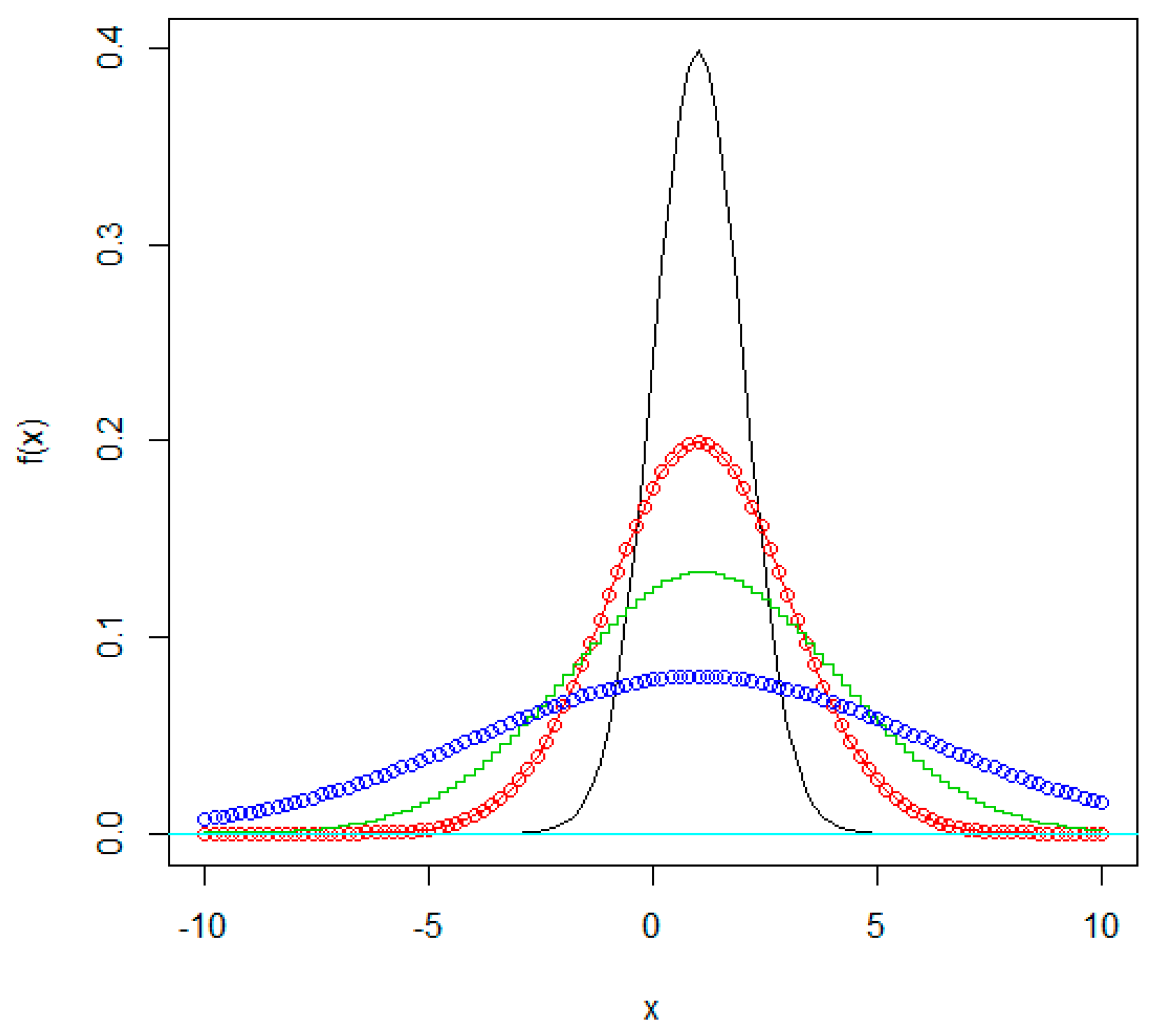
Figure 1. Probability density function (PDF) of normal ( μ , σ 2 ) distribution with different coefficient of variation (CV) values. Black: μ = 1 ,   σ = 1 , CV = 1; red: μ = 1 ,   σ = 2 , CV = 2; green: μ = 1 ,   σ = 3 , CV = 3; blue: μ = 1 ,   σ = 5 , CV = 5.
Symmetry 11 00824 g001
Figure 2. PDF of gamma ( α , λ ) distribution with different CV values. Black:   α = 1 , λ = 0.001 , CV = 1; red: α = 0.25 , λ = 0.001 , CV = 2; green: α = 0.11 , λ = 0.001 , CV = 3; blue: α = 0.04 ,   λ = 0.001 , CV = 5.
Symmetry 11 00824 g002
Figure 3. PDF of beta ( α , β ) distribution with different CV values. Black: α = 0.94 , β = 30.39 , CV = 1; red: α = 0.21 , β = 6.87 , CV = 2; green: α = 0.08 , β = 2.51 , CV = 3; blue: α = 0.009 ,   β = 0.285 , CV = 5.
Symmetry 11 00824 g003
Figure 4. Q-Q plots to study the normality of the introduced test statistic.
Symmetry 11 00824 g004
Table 1. The CP values for different parameter settings.
( m , n )
D i s t r i b u t i o n ( C V X , C V Y ) ( 50 , 100 ) ( 75 , 100 ) ( 100 , 200 ) ( 200 , 300 ) ( 500 , 700 ) ( 700 , 1000 )
Normal ( 1 , 1 ) 0.945 0.947 0.951 0.953 0.959 0.960
( 1 , 2 ) 0.945 0.948 0.952 0.953 0.958 0.959
( 2 , 3 ) 0.944 0.948 0.953 0.953 0.959 0.961
( 2 , 5 ) 0.946 0.950 0.950 0.955 0.956 0.960
Gamma ( 1 , 1 ) 0.946 0.948 0.952 0.956 0.958 0.961
( 1 , 2 ) 0.947 0.949 0.951 0.954 0.958 0.961
( 2 , 3 ) 0.947 0.950 0.952 0.953 0.959 0.961
( 2 , 5 ) 0.945 0.949 0.952 0.956 0.958 0.962
Beta ( 1 , 1 ) 0.944 0.950 0.950 0.954 0.958 0.961
( 1 , 2 ) 0.946 0.948 0.952 0.954 0.957 0.960
( 2 , 3 ) 0.945 0.947 0.952 0.954 0.958 0.959
( 2 , 5 ) 0.945 0.948 0.951 0.954 0.956 0.960
Table 2. The CPU times for running the introduced approach.
( m , n )
D i s t r i b u t i o n ( C V X , C V Y ) ( 50 , 100 ) ( 75 , 100 ) ( 100 , 200 ) ( 200 , 300 ) ( 500 , 700 ) ( 700 , 1000 )
Normal ( 1 , 1 ) 8.64 10.08 14.08 23.09 51.92 68.67
( 1 , 2 ) 8.72 10.29 16.41 21.85 52.19 74.17
( 2 , 3 ) 9.52 9.50 15.42 21.10 51.05 65.87
( 2 , 5 ) 9.35 10.90 15.25 24.31 49.97 74.90
Gamma ( 1 , 1 ) 9.45 9.02 15.16 22.13 47.05 74.92
( 1 , 2 ) 8.00 9.58 14.65 24.87 49.96 66.20
( 2 , 3 ) 9.63 9.29 14.47 21.91 52.52 66.84
( 2 , 5 ) 8.69 9.83 16.29 24.27 50.68 66.11
Beta ( 1 , 1 ) 9.53 10.57 14.19 21.47 53.26 66.58
( 1 , 2 ) 9.20 9.50 14.15 24.85 48.67 75.00
( 2 , 3 ) 9.02 9.63 14.25 23.52 50.29 69.67
( 2 , 5 ) 8.75 9.17 15.73 22.89 50.79 73.95
Table 3. P-values for studying the normality of the introduced test statistic.
( m , n )
D i s t r i b u t i o n ( C V X , C V Y ) ( 50 , 100 ) ( 75 , 100 ) ( 100 , 200 ) ( 200 , 300 ) ( 500 , 700 ) ( 700 , 1000 )
Normal ( 1 , 1 ) 0.444 0.551 0.662 0.701 0.899 0.977
( 1 , 2 ) 0.432 0.580 0.656 0.795 0.860 0.982
( 2 , 3 ) 0.408 0.600 0.602 0.718 0.859 0.943
( 2 , 5 ) 0.481 0.569 0.681 0.740 0.848 0.955
Gamma ( 1 , 1 ) 0.428 0.545 0.677 0.760 0.851 0.905
( 1 , 2 ) 0.407 0.544 0.612 0.775 0.880 0 , 909
( 2 , 3 ) 0.484 0.508 0.611 0.708 0.855 0.940
( 2 , 5 ) 0.494 0.556 0.647 0.754 0.800 0.978
Beta ( 1 , 1 ) 0.411 0.599 0.657 0.709 0.870 0.946
( 1 , 2 ) 0.489 0.585 0.652 0.763 0.841 0.978
( 2 , 3 ) 0.411 0.505 0.606 0.724 0.874 0.908
( 2 , 5 ) 0.461 0.527 0.671 0.757 0.847 0.933