1. Introduction
In many situations, we aim to study the effects of variables
on variable
. Simple and multiple regressions are data analysis techniques to model these effects. The authors of the references [
1,
2] applied simple and multiple linear regression models in different science fields, such as agriculture, biology, material, mechanical engineering, and signal processing. In many real world problems, scientists want to compare the relationship between the dependent variable and independent variables in several separate datasets.
The comparison of the correlation between the variables X and Y in two separate datasets, different techniques was provided by [
3,
4,
5]. The comparison of the correlation between the variables X and Y in a dataset, and the correlation between the two variables X and W in another dataset, resulted in different methods developed by [
6,
7,
8,
9,
10]. The correlation between the variables X and Y in a dataset, and the correlation between two variables W and Z in another dataset, were compared by different methods in [
9,
11,
12]. The comparison and classification of two, and more simple linear regression models, have been considered in [
13,
14,
15,
16]. The comparison of two regression models has been reported in [
14,
15,
16,
17,
18,
19,
20,
21,
22].
In the present research, we aim to compare and classify several linear and non-linear regression models that fitted on several independent datasets. The non-parametric methods are used to construct an approach to investigate the similarity and to classify the linear and non-linear regression models. A given approach is then evaluated using simulation and real world studies. The introduced approach is powerful and applicable in its ability to compare any linear or non-linear regression models.
2. Models Comparing and Classification
Assume
is a sample dataset of size
, from
The equations of
m linear or non-linear regression models can be written by:
such that for
are zero-mean symmetric random variables with unknown and equal variance
.
By considering Equation (1), consequently, the conditional expectation of Y based on
that we show it by
is given by:
In real-word problems the aim is to test the hypothesis Under the rejection of , we conclude that at least two models of the m regression models are not statistically similar, and if is accepted then it can be concluded that the m regression models are statistically equal.
The regression equations can be represented by:
such that
are the values for the dependent variable Y,
are the values for the independent variables
,
and
are zero-mean random variables with unknown and equal variance
.
First, all
m regression models are estimated by
for all
values of
, where
are the estimated values for dependent variable
, based on ith regression model. Since
are zero-mean symmetric random variables, consequently,
are unbiased estimators for
respectively. In other words,
are random variables with mean
Remark 1. means that the repeated points are assumed once.
Now, to compare the fitted regression models, the Friedman test [
23,
24,
25,
26] will be applied on
n couples
The Friedman test that is a non-parametric alternative to the repeated measures is used to compare related datasets (datasets that are repeated on the same subjects). This test is commonly applied when dataset do not follow the parametric conditions, such as normality assumption.
Classification
In previous discussion, if is false, then we conclude that the mechanism of one model or mechanisms of some models are significantly different from the other models. However, to determine which models are significantly different from each other, the sign test or Wilcoxon test are applied in order to compare each of the regression model pairs.
3. Simulation Study
This section assesses the ability of the introduced approach simulation datasets. First, the different datasets from different regression models are produced. Then, we compute the values of the Estimated Type I error probability () and the Estimated Power of the introduced approach. For comparison, the Wilcoxon and Friedman tests are applied. The simulations are accomplished after 1000 runs and using the R 3.5.3 software (R Development Core Team, 2018) on a PC (Processor: Intel(R) CoreTM(2) Duo CPU T7100 @ 1.80GHz 1.80GHz, RAM: 2.00GB, System Type: 32-bit).
Example 1. Assume the simple linear regression model:such that and are independent. Example 2. Letsuch that and are independent. Example 3. Assume:such that and are independent. Example 4. Assume the multiple linear regression model:such that , and are independent. Example 5. For the first dataset, assume the simple nonlinear regression model:such that and are independent. For the second and the third datasets let and respectively.
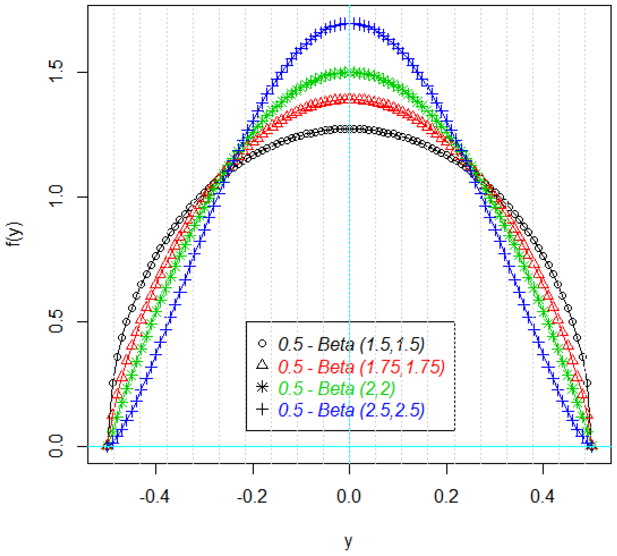
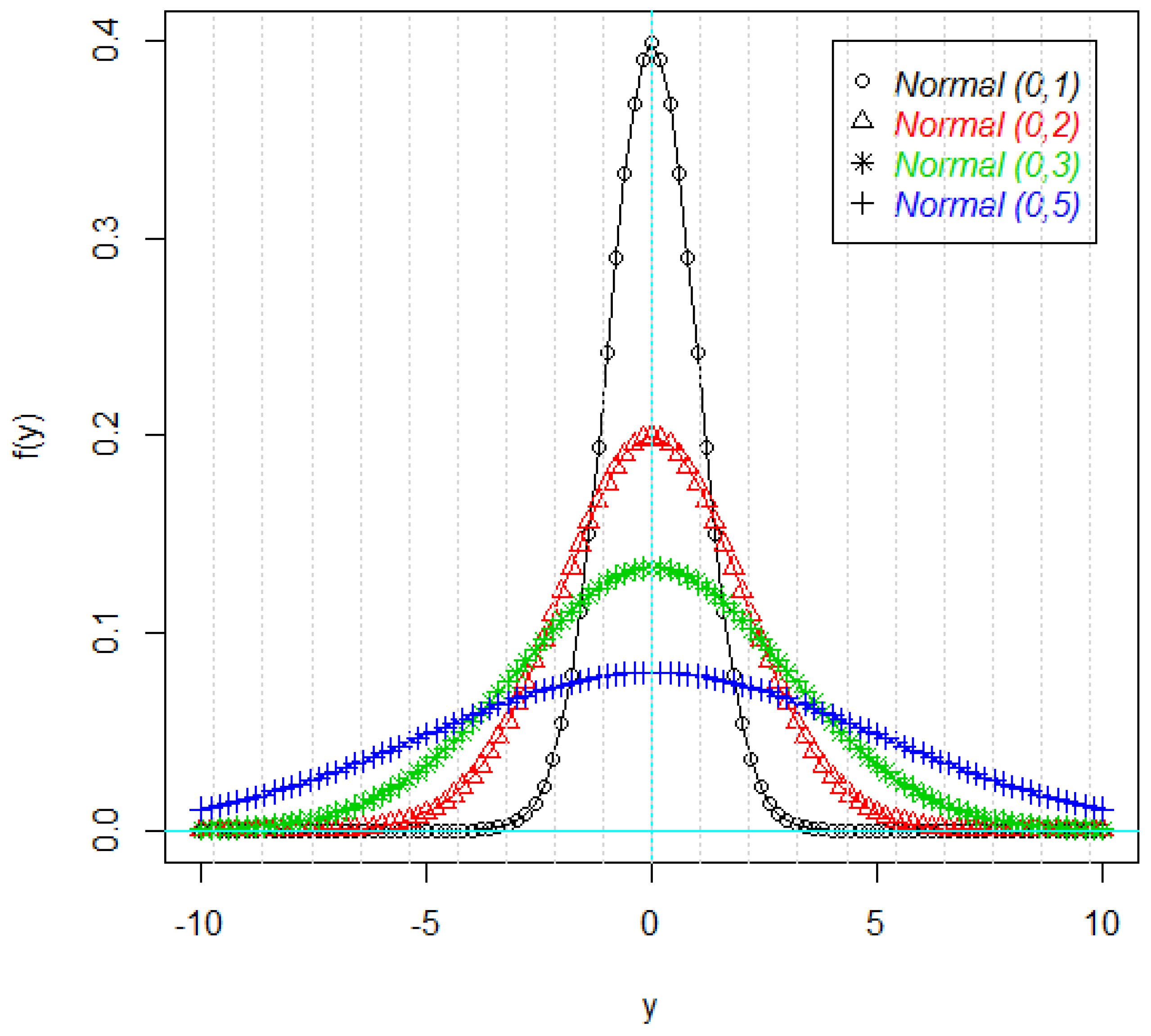
Figure 1 and
Figure 2 shows the density plots of the some parts of the response variable Y. As it can be seen in these figures, the density plots are symmetric, but not necessarily normal (
Figure 2).
The values of
(first four rows) and
(other rows) for Examples 1 to 5 are summarized in
Table 1,
Table 2,
Table 3,
Table 4 and
Table 5, respectively. As
Table 1,
Table 2,
Table 3,
Table 4 and
Table 5 indicate the values of
are very close to size test (
0.05), and consequently the introduced approach can be controlled the type I error. Also the values of
show that the given technique can distinguished between the null and alternative hypotheses.
4. Real Data
In this section, a practical real data is considered to study the power of the introduced approach in real world problems. Drought is a damaging natural phenomenon. To prevent this phenomenon, the hydrologists model and predict the drought datasets in a standard time period. In this research, the average monthly rainy days (1966–2010) at three Iranian synoptic stations (Fasa, Sarvestan, and Shiraz) was considered and modeled.
To model and forecast the average monthly rainy days, different polynomial regression models of orders 1 to 3 (linear, quadratic and cubic) and exponential model were fitted to datasets. The formulas of the considered models are as following:
Linear model:
Quadratic model:
The numerical computations are done using the R 3.5.3 software (Library ‘nlstools’, lm() function for linear regression and nls() function for nonlinear regression) and Minitab 18 software.
The results of fitted regression models are summarized in
Table 6. It can be observed that, for all of the stations, respectively, the polynomial regression of order 3 (cubic), and the exponential models, had the most R-square (
R2) and the least root mean square error (
RMSE) between all fitted models.
Now, we use the proposed approach to compare and classify these stations, for each model. The result of Friedman test is shown in
Table 7. This table indicated that the fitted cubic and exponential models are significantly different in these stations (
p < 0.05). Also, there is no significant difference between the fitted linear and quadratic models in these stations (
p > 0.05).
As
Table 8 indicates, we can classify the stations in two clusters, for cubic and exponential models. First cluster: Fasa and Sarvestan, and second cluster: Shiraz.
5. Conclusions
In many real world problems, researchers wish to compare and classify the regression models in several datasets. In this paper, the non-parametric methods were used to construct an approach to investigate the similarity of some linear and non-linear regression models with symmetric errors. Particular approaches were evaluated using simulation and practical datasets. A simulation study indicated that the introduced approach controlled the Type I error. Also the proposed technique distinguished well between null and alternative hypotheses. The introduced approach also had many advantages. First, it was powerful. Second, it was not too computational. Third, it could be applied to compare any linear or non-linear regression models. Fourth, this method did not need the normality of errors and could be applied for all models with symmetric errors.
Author Contributions
Conceptualization, J.-J.P., M.R.M. and D.B.; Formal analysis, M.R.M., D.B. and M.M.; Investigation, J.-J.P., M.R.M. and D.B.; Methodology, J.-J.P., M.R.M., D.B. and M.M.; Project administration, J.-J.P.; Software, J.-J.P., M.R.M., D.B. and M.M.; Supervision, J.-J.P., M.R.M. and D.B.; Validation, J.-J.P., M.R.M. and D.B.; Visualization, J.-J.P., M.R.M. and D.B.; Writing—Original Draft, J.-J.P. and M.R.M.; Writing—Review and Editing, J.-J.P., M.R.M., D.B. and M.M.
Funding
This research received no external funding.
Conflicts of Interest
The authors declare no conflict of interest.
References
- Wan, J.; Zhang, D.; Xu, W.; Guo, Q. Parameter Estimation of Multi Frequency Hopping Signals Based on Space-Time-Frequency Distribution. Symmetry 2019, 11, 648. [Google Scholar] [CrossRef]
- Sajid, M.; Shafique, T.; Riaz, I.; Imran, M.; Jabbar Aziz Baig, M.; Baig, S.; Manzoor, S. Facial asymmetry-based anthropometric differences between gender and ethnicity. Symmetry 2018, 10, 232. [Google Scholar] [CrossRef]
- Mahmouudi, M.R.; Maleki, M.; Pak, A. Testing the Difference between Two Independent Time Series Models. Iran. J. Sci. Technol. Trans. A Sci. 2017, 41, 665–669. [Google Scholar] [CrossRef]
- Fisher, R.A. On the Probable Error of a Coefficient of Correlation Deduced from a Small Sample. Metron 1921, 1, 3–32. [Google Scholar]
- Mahmoudi, M.R.; Mahmoodi, M. Inferrence on the Ratio of Correlations of Two Independent Populations. J. Math. Ext. 2014, 7, 71–82. [Google Scholar]
- Howell, D.C. Statistical Methods for Psychology, 6th ed.; Thomson Wadsworth: Stamford, CT, USA, 2007. [Google Scholar]
- Hotelling, H. The Selection of Variates for Use in Prediction with Some Comments on the General Problem of Nuisance Parameters. Ann. Math. Stat. 1940, 11, 271–283. [Google Scholar] [CrossRef]
- Williams, E.G. The Comparison of Regression Variables. J. R. Stat. Soc. Ser. B 1959, 21, 396–399. [Google Scholar] [CrossRef]
- Steiger, J.H. Tests for Comparing Elements of a Correlation Matrix. Psychol. Bull. 1980, 87, 245–251. [Google Scholar] [CrossRef]
- Meng, X.; Rosenthal, R.; Rubin, D.B. Comparing Correlated Correlation Coefficients. Psychol. Bull. 1992, 111, 172–175. [Google Scholar] [CrossRef]
- Peter, C.C.; Van Voorhis, W.R. Statistical Procedures and Their Mathematical Bases; McGraw-Hill: New York, NY, USA, 1940. [Google Scholar]
- Raghunathan, T.E.; Rosenthal, R.; Rubin, D.B. Comparing Correlated but Nonoverlapping Correlations. Psychol. Methods 1996, 1, 178–183. [Google Scholar] [CrossRef]
- Liu, W.; Jamshidian, M.; Zhang, Y. Multiple Comparison of Several Linear Regression Lines. J. R. Stat. Soc. Ser. B 2004, 99, 395–403. [Google Scholar]
- Liu, W.; Hayter, A.J.; Wynn, H.P. Operability Region Equivalence: Simultaneous Confidence Bands for the Equivalence of Two Regression Models Over Restricted Regions. Biom. J. 2007, 49, 144–150. [Google Scholar] [CrossRef] [PubMed]
- Liu, W.; Jamshidian, M.; Zhang, Y.; Bertz, F.; Han, X. Pooling Batches in Drug Stability Study by Using Constant-width Simultaneous Confidence Bands. Stat. Med. 2007, 26, 2759–2771. [Google Scholar] [CrossRef] [PubMed]
- Liu, W.; Jamshidian, M.; Zhang, Y.; Bertz, F.; Han, X. Some New Methods for the Comparison of Two Linear Regression Models. J. Stat. Plan. Inference 2007, 137, 57–67. [Google Scholar] [CrossRef]
- Hayter, A.J.; Liu, W.; Wynn, H.P. Easy-to-Construct Confidence Bands for Comparing Two Simple Linear Regression Lines. J. Stat. Plan. Inference 2007, 137, 1213–1225. [Google Scholar] [CrossRef]
- Jamshidian, M.; Liu, W.; Bretz, F. Simultaneous Confidence Bands for all Contrasts of Three or More Simple Linear Regression Models over an Interval. Comput. Stat Data Anal. 2010, 54, 1475–1483. [Google Scholar] [CrossRef]
- Marques, F.J.; Coelho, C.A.; Rodrigues, P.C. Testing the equality of several linear regression models. Comput. Stat. 2016, 32, 1453–1480. [Google Scholar] [CrossRef]
- Mahmoudi, M.R.; Mahmoudi, M.; Nahavandi, E. Testing the Difference between Two Independent Regression Models. Commun. Stat. Theory Methods 2016, 45, 6284–6289. [Google Scholar] [CrossRef]
- Mahmoudi, M.R. On Comparing Two Dependent Linear and Nonlinear Regression Models. J. Test. Eval. 2018, 47, 449–458. [Google Scholar] [CrossRef]
- Mahmoudi, M.R.; Maleki, M.; Pak, A. Testing the Equality of Two Independent Regression Models. Commun. Stat. Theory Methods 2018, 47, 2919–2926. [Google Scholar] [CrossRef]
- Conover, W.J. Practical Nonparametric Statistics, 3rd ed.; John Wiley: Hoboken, NJ, USA, 1980. [Google Scholar]
- Friedman, M. The Use of Ranks to Avoid the Assumption of Normality Implicit in the Analysis of Variance. J. R. Stat. Soc. Ser. B 1937, 32, 675–701. [Google Scholar] [CrossRef]
- Friedman, M. A Correction: The Use of Ranks to Avoid the Assumption of Normality Implicit in the Analysis of Variance. J. R. Stat. Soc. Ser. B 1939, 34, 109. [Google Scholar] [CrossRef]
- Friedman, M. A Comparison of Alternative Tests of Significance for the Problem of m Rankings. Ann. Math. Stat. 1940, 11, 86–92. [Google Scholar] [CrossRef]
© 2019 by the authors. Licensee MDPI, Basel, Switzerland. This article is an open access article distributed under the terms and conditions of the Creative Commons Attribution (CC BY) license (http://creativecommons.org/licenses/by/4.0/).


