LPI Radar Waveform Recognition Based on CNN and TPOT

Abstract

The electronic reconnaissance system is the operational guarantee and premise of electronic warfare. It is an important tool for intercepting radar signals and providing intelligence support for sensing the battlefield situation. In this paper, a radar waveform automatic identification system for detecting, tracking and locating low probability interception (LPI) radar is studied. The recognition system can recognize 12 different radar waveform: binary phase shift keying (Barker codes modulation), linear frequency modulation (LFM), Costas codes, polytime codes (T1, T2, T3, and T4), and polyphase codes (comprising Frank, P1, P2, P3 and P4). First, the system performs time–frequency transform on the LPI radar signal to obtain a two-dimensional time–frequency image. Then, the time–frequency image is preprocessed (binarization and size conversion). The preprocessed time–frequency image is then sent to the convolutional neural network (CNN) for training. After the training is completed, the features of the fully connected layer are extracted. Finally, the feature is sent to the tree structure-based machine learning process optimization (TPOT) classifier to realize offline training and online recognition. The experimental results show that the overall recognition rate of the system reaches 94.42% when the signal-to-noise ratio (SNR) is −4 dB.

1. Introduction

In recent years, low probability interception (LPI) radars have been widely used on the battlefield due to their difficulty in being intercepted by non-cooperative receivers. Unlike traditional radar signals, LPI radars have low power, large bandwidth, and frequency changes, giving them powerful combat capabilities and good survivability [1,2,3,4]. At present, how to accurately identify LPI radar waveforms at low SNR has become an important issue in the field of radar countermeasures.

The key to LPI radar waveform recognition is feature extraction and classifier design. In [5], Choi–Williams Distribution (CWD) is used to process radar signals in time and frequency. Then, useful features are extracted by image processing. Five kinds of waveform recognition, namely BPSK, FMCW (Frequency Modulation Continuous Wave), Frank code, P4 code and T1 code, are realized. Under the condition of SNR = 0 dB, the recognition success rate is greater than 80%. Author1 [6] used the algorithm based on random projection and sparse classification to recognize LFM, FSK and PSK. At the signal-to-noise ratio of 0 dB, the recognition success rate is over 90%. Lunden solved eight radar waveforms (LFM, BPSK, Costas, Frank code, and P1–P4 code) based on CWD and Wigner–Ville Distribution (WVD) processing, and achieved good recognition performance at lower SNR [7]. However, the algorithm needs to estimate the carrier frequency and the sub-pulse width. In a complex noise environment, the inaccurate parameter estimation leads to a decrease in the recognition success rate. Author1 [8] proposed many potential features based on CWD and WVD, and discardrf redundant features through feature selection algorithm of information theory. According to MLP network, the recognition rate reaches 98% when SNR is −6 dB. In [9], Ming proposed a hybrid classifier, including two relatively independent sub-networks of Convolutional Neural Network (CNN) and Herman Neural Network (ENN). Under the condition of SNR of −2 dB, the overall recognition rate of 12 kinds of signals reaches 94.5%. In [10], Shuang proposed a radar waveform recognition method based on time–frequency image and artificial bee colony optimization support vector machine. The experimental results show that the recognition rate of the eight types of LPI radar signals reaches 92% when the SNR is −4 dB. Therefore, how to identify more types of LPI radar waveforms at low SNR is a challenge for existing methods.

In summary, to solve the problem of LPI radar signal feature extraction and low recognition rate of multiple types of radar waveforms, this paper proposes an LPI radar waveform recognition system based on convolutional neural network and TPOT. The system identifies 12 types of LPI radar waveforms: BPSK, Costas code, LFM, P1–P4, Frank code, and T1–T4. The system consists of four parts: LPI radar waveform time–frequency analysis, time–frequency image preprocessing, CNN and TPOT. First, the detected LPI radar waveform is subjected to CWD time–frequency transform, and the one-dimensional time signal is converted into a two-dimensional time–frequency image. The time–frequency image is then pre-processed to convert the time–frequency image into the format required for CNN input. Then, the pre-processed 2D time–frequency image is sent to the CNN for training and extracting the full connection layer feature. Finally, the feature is sent to the tree structure-based machine learning process optimization (TPOT) classifier to realize offline training and online recognition.

The structure of this paper is organized as follows. Section 2 presents is the overall structure of the system. Section 3 proposes the signal model and preprocessing. Section 4 designs the CNN feature extraction model. Section 5 designs TPOT selection and optimizes the classifier. Section 6 creates a simulation experiment and discusses the simulation results. Section 7 draws the conclusion.

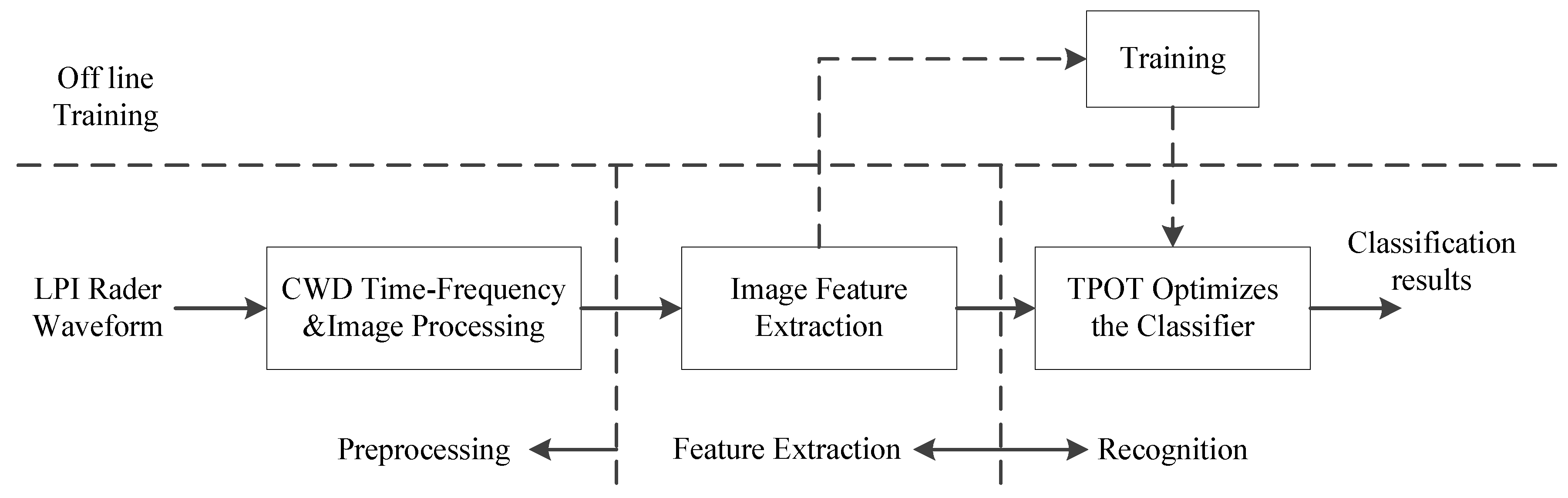
2. CNN-TPOT Identification System Structure

The CNN-TPOT radar identification system in this paper consists of three parts: preprocessing, feature extraction and recognition. First, in the preprocessing part, the received LPI radar waveform data are time–frequency transformed to obtain a two-dimensional time–frequency image of the signal. Then, the time–frequency image is binarized and the image size is transformed, and the two-dimensional time–frequency images are converted into a binary image. In the feature extraction part, the partially preprocessed image is first selected as the training data, and the remainder is used as the test data to train the CNN and save the model. Then, the last fully connected layer data of CNN extracts the radar waveform feature. In the recognition part, firstly, feature normalization is processed, and then dimensionality reduction is processed by PCA (Principal Components Analysis) algorithm. The training data features are sent to the TPOT to select and optimize the classifier parameters. Finally, the test data features are sent to the TPOT optimized classifier to obtain the LPI radar waveform recognition results. See Figure 1 for details.

3. Preprocessing

In this section, the detected LPI radar waveform is first converted into a two-dimensional time–frequency image by CWD time–frequency analysis, then the time–frequency image is binarized, and finally the binarized image is converted into an image suitable for CNN input.

3.1. Signal Model

In this paper, the center frequency of the signal bandwidth is considered as carrier frequency. In addition, the signal is disturbed by additive white Gaussian noise, which means that the intercepted discrete time signal model is given by [11]

$$y\left(nT\right)=s\left(nT\right)+m\left(nT\right)=A{e}^{j\varphi \left(nT\right)}+m\left(nT\right)$$

(1)

where n is an integer, T is the sampling interval, and $s\left(nT\right)$ is the complex signal of the transmitted signal. $m\left(nT\right)$ is a complex Gaussian white noise with a variance of ${\sigma }_{ϵ}^2$. Usually, we assume $A=1$. $\varphi$ is the instantaneous phase. The detected signal is processed from the real signal to the complex signal using the Hilbert transform [12].

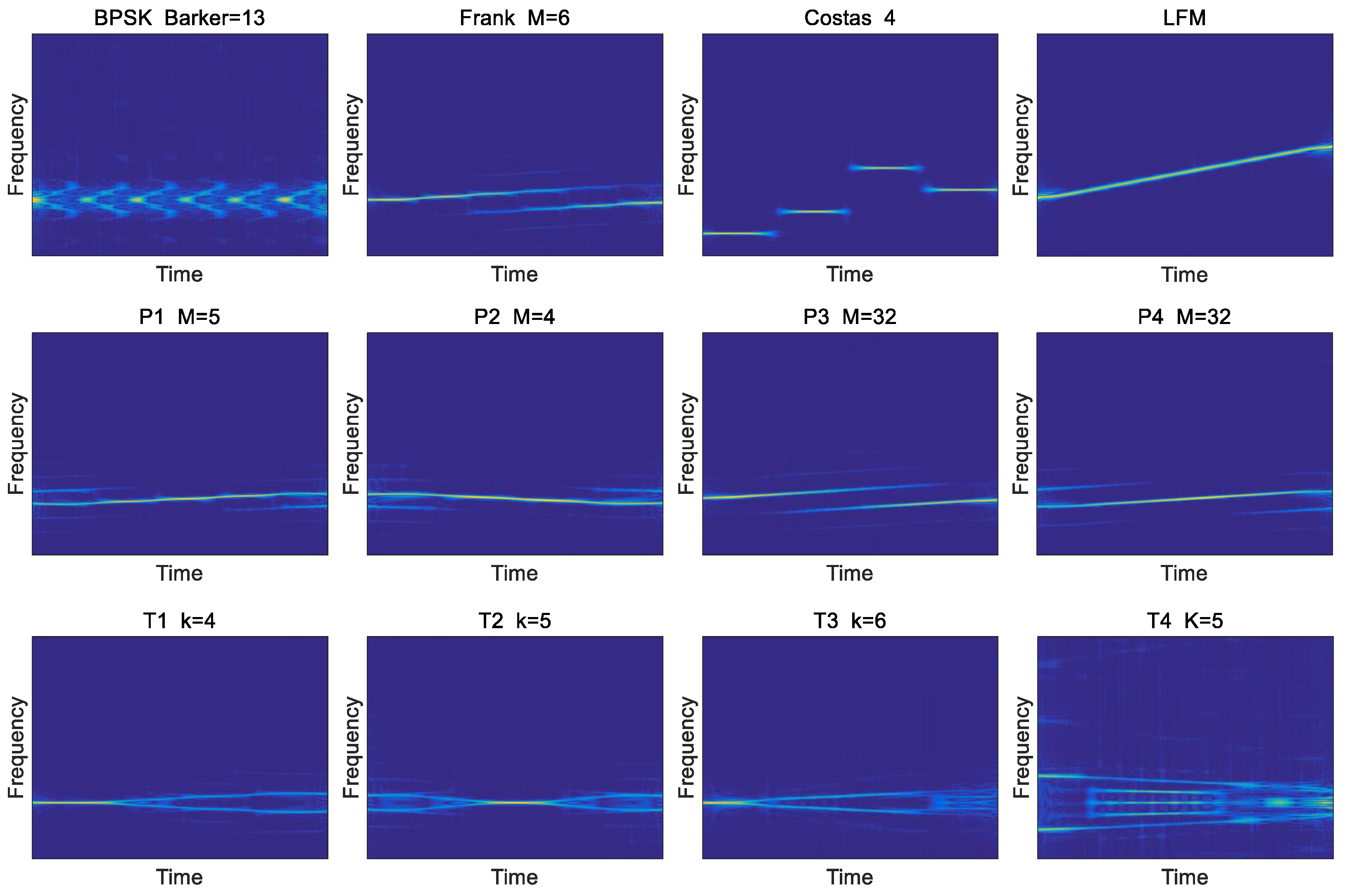
3.2. Choi–Williams Distribution

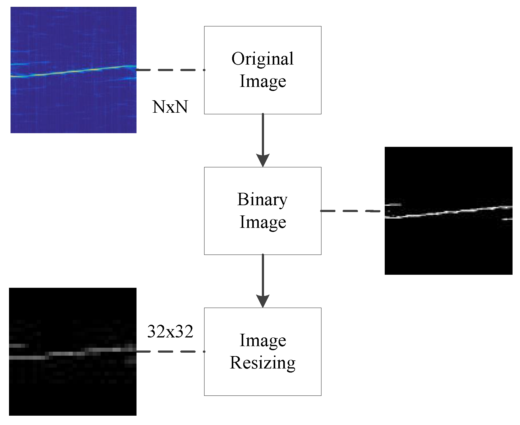
Choi–Williams distribution is a kind of time–frequency transformation which is an effective approach to preventing the cross terms [13,14].

$$C(\omega ,t)=\int \int \int f(\xi ,\tau )e^{j2\pi \xi (s-t)}x(s+\tau /2)x^{*}(s-\tau /2)e^{-j\omega \tau }$$

(2)

where $C(\omega ,t)$ is the result of time–frequency transform. $\omega$ and t are frequency and time, respectively. $f(\xi ,\tau )$ is a kernel function, as follows.

$$f(\xi ,\tau )=e^{{\left(\pi \xi \tau \right)}^2/2\sigma }$$

(3)

The kernel function is a low-pass filter in two-dimensional space and has the effect of eliminating cross terms. $\sigma$ is a controllable factor that determines the bandwidth of the filter. In this paper, we set the $\sigma =1$ balance cross term and resolution. Figure 2 shows the results of the CWD transformation of the twelve LPI radar signals. We found a way to improve the speed of CWD calculations in [15]. In this paper, 1024 × 1024 CWD points are selected.

3.3. Binary Image

Since the system is more concerned with the shape of the radar waveform on the time–frequency image than the signal energy, the radar waveform time–frequency map can be converted into a black-and-white binary image by binarization processing. This can reduce the influence of noise and simplify the calculation of the identification part. In this section, we use the full threshold binarization method to process the image [16]. The global binarization threshold selection steps are as follows.

• Get the probability of occurrence of each gray value that appears in the picture. For example, $PPix(0,i)$ stores the gray value of the ith pixel in the image, and $PPix(1,i)$ stores the probability that the ith gray value appears.
• Calculate the discrete function distribution $F\left(i\right)$ of the gray value.

  $$F\left(i\right)={\displaystyle \sum _{j=0}^i}PPix(0,j)\times PPix(1,j)$$

  (4)

  where i is the total number of types of gray values from zero to the image.
• Find the sum of the probabilities of the occurrence of the previous i kinds of gray values, $PSum\left(i\right)$.
• Obtain the gray average value AGray of the overall image, that is, sum the gray value of all the pixels in the image and then divide by the total number of pixels.
• Calculate the threshold weight $WValve\left(i\right)$ at different gray values.

  $$WValve\left(i\right)=\frac{AGray\times F\left(i\right)-PSum\left(i\right)}{\sqrt{F\left(i\right)\times (1-F(i\left)\right)}}$$

  (5)
• Obtain the gray value corresponding to the i value of the maximum $WValve\left(i\right)$ as a global binarization threshold.

After the time–frequency image is binarized, the binarized image is size-converted and adjusted to match the pixel size of the CNN input. Figure 3 shows the time–frequency image pre-processing flow. The time–frequency image of the final pre-processing is shown in Figure 4.

4. CNN Feature Extractor Design

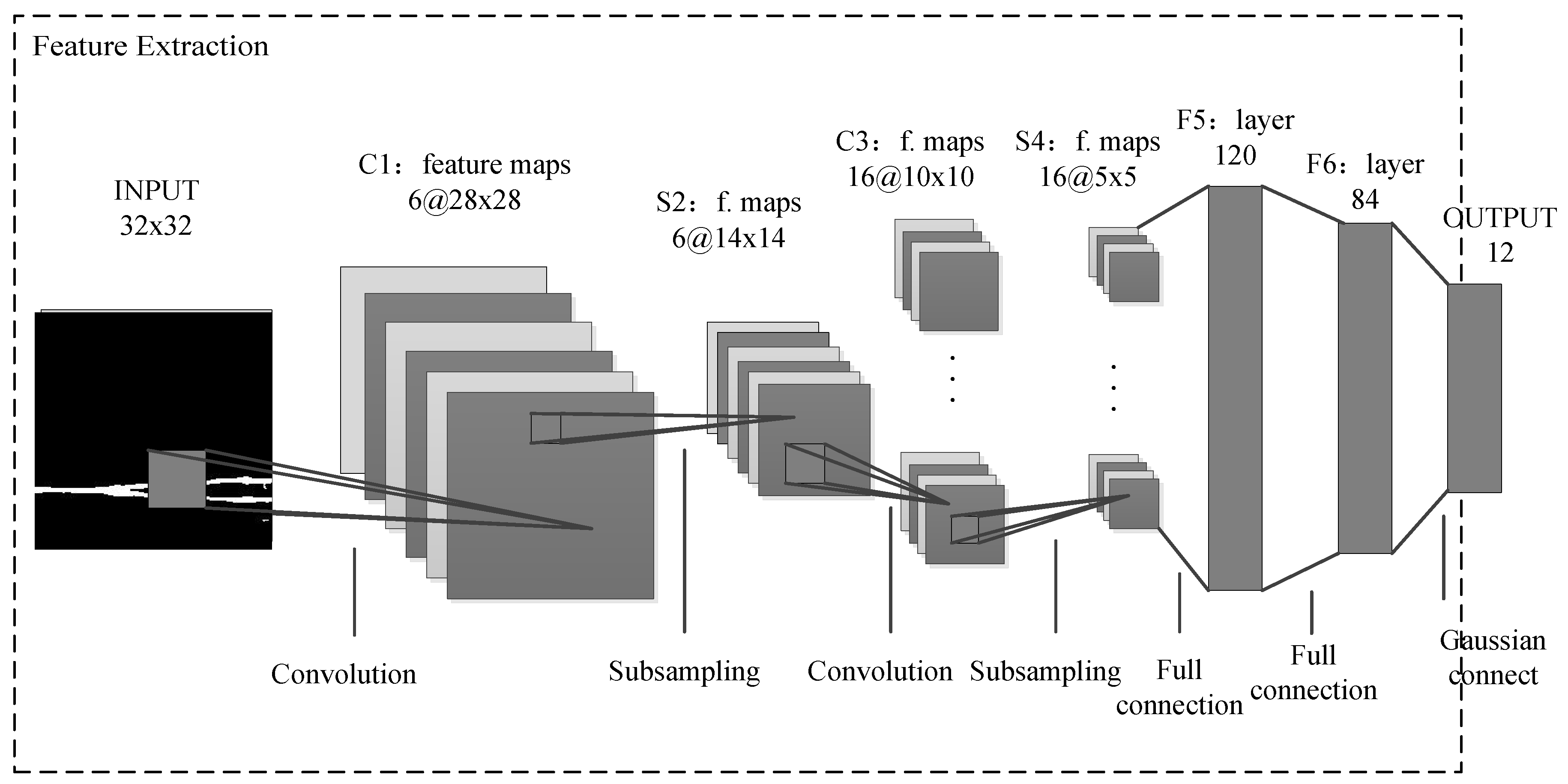
This section mainly introduces the structure of the CNN training model and the feature extraction of the LPI radar waveform. Details as follows.

4.1. CNN Model

CNN has a special feature extraction structure [17,18,19,20]. The CNN input two-dimensional picture, the output is the probability of classification results. This section first designs the complete CNN structure and then sends the training dataset to the training data training network. Finally, the last layer of the fully connected layer of the network is removed, and the data of the last layer of the fully connected layer are extracted as a feature. The CNN model structure is shown in Figure 5. The specific structure of CNN is described below.

• The input image is a standardized CNN training data structure with a size of $32\times 32$. The detected LPI radar waveform is subjected to CWD time–frequency transform and image binarization. However, since the image size is too large to train the CNN network, we use image size conversion to $32\times 32$ size.
• The C1 layer is a convolutional layer with six feature maps. The size of the convolution kernel is $5\times 5$, thus each feature map has $(32-5+1)\times (32-5+1)$, i.e., $28\times 28$ Neurons. Each neuron is connected to a $5\times 5$ size region of the input layer.
• The S2 layer is a down sampling layer with six $14\times 14$ feature maps, and each neuron in each feature map is connected to a $2\times 2$ region in the feature map corresponding to the C1 layer.
• C3 is also a convolutional layer that uses a $5\times 5$ convolution kernel to process the S2 layer. The number of neurons that calculate the feature map of the C3 layer is $(14-5+1)\times (14-5+1)$, that is, $10\times 10$. C3 has 16 feature maps, each of which is composed of different combinations between the individual feature maps of the previous layer, as shown in

  Table 1. The CNN third layer feature map combination; for example, the 0th feature map is obtained by combining the zero-feature, one-feature and two-feature maps of the S2 layer.

  	0	1	2	3	4	5	6	7	8	9	10	11	12	13	14	15
  0	X				X	X	X			X	X	X	X		X	X
  1	X	X				X	X	X	X		X	X	X	X		X
  2	X	X	X				X	X	X			X		X	X	X
  3		X	X	X			X	X	X	X	X		X		X	X
  4			X	X	X			X	X	X	X		X	X		X
  5				X	X	X			X	X	X	X		X	X	X

  .
• The S4 layer is a down sampling layer composed of 16 $5\times 5$ size feature maps, each of which is connected to a $2\times 2$ size region of the corresponding feature map in C3.
• The C5 layer is another convolutional layer. The same is used for a $5\times 5$ size convolution kernel. Each feature map has $(5-5+1)\times (5-5+1)$, i.e., $1\times 1$ neurons. Each unit is fully connected to the $5\times 5$ area of all 16 feature maps of S4. The C5 layer has 120 feature maps.
• The F6 fully connected layer has 84 feature maps, and each feature map has only one neuron connected to the C5 layer.
• The output layer is also a fully connected layer with a total of 12 nodes representing the 12 different LPI radar waveforms, respectively.

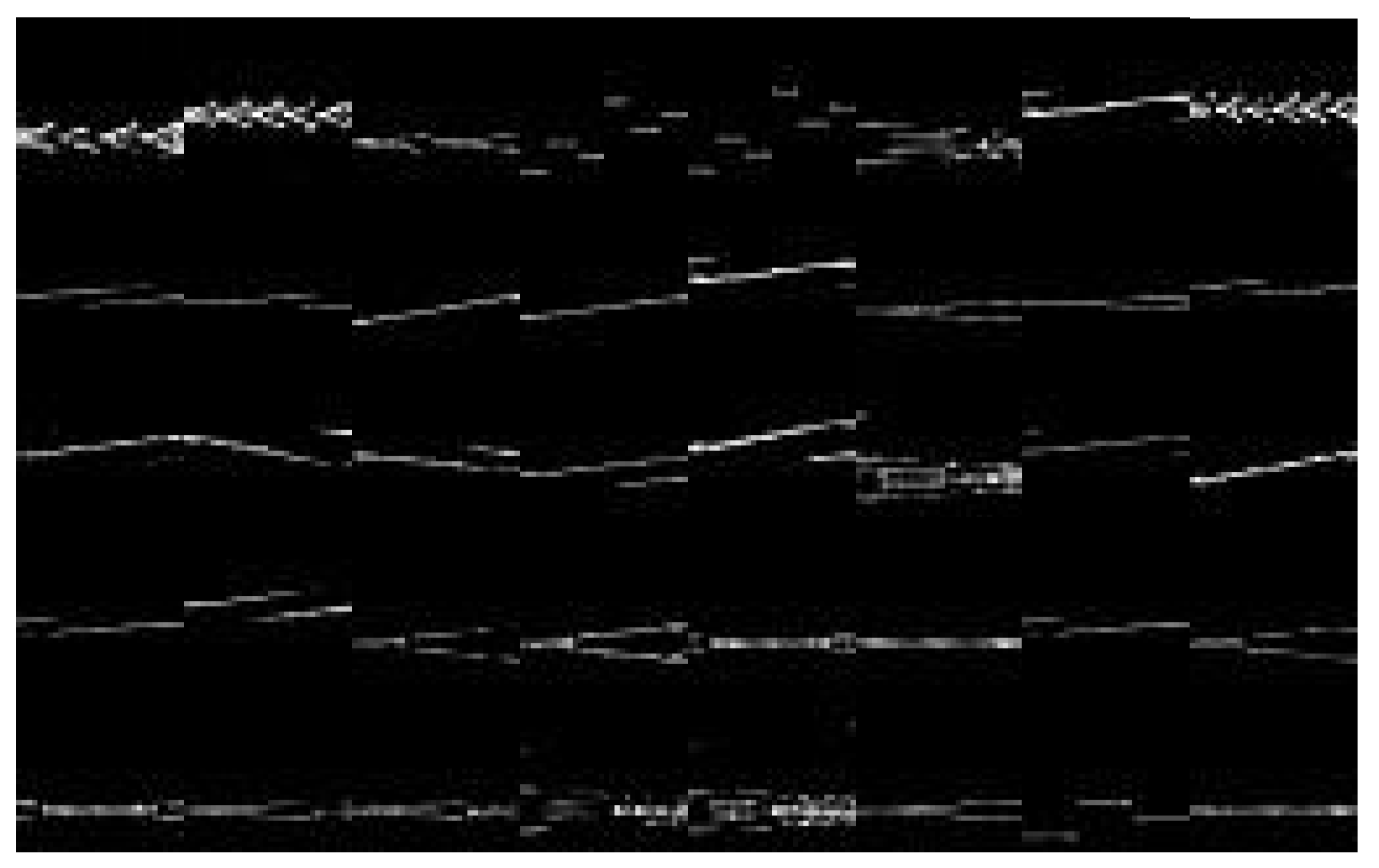
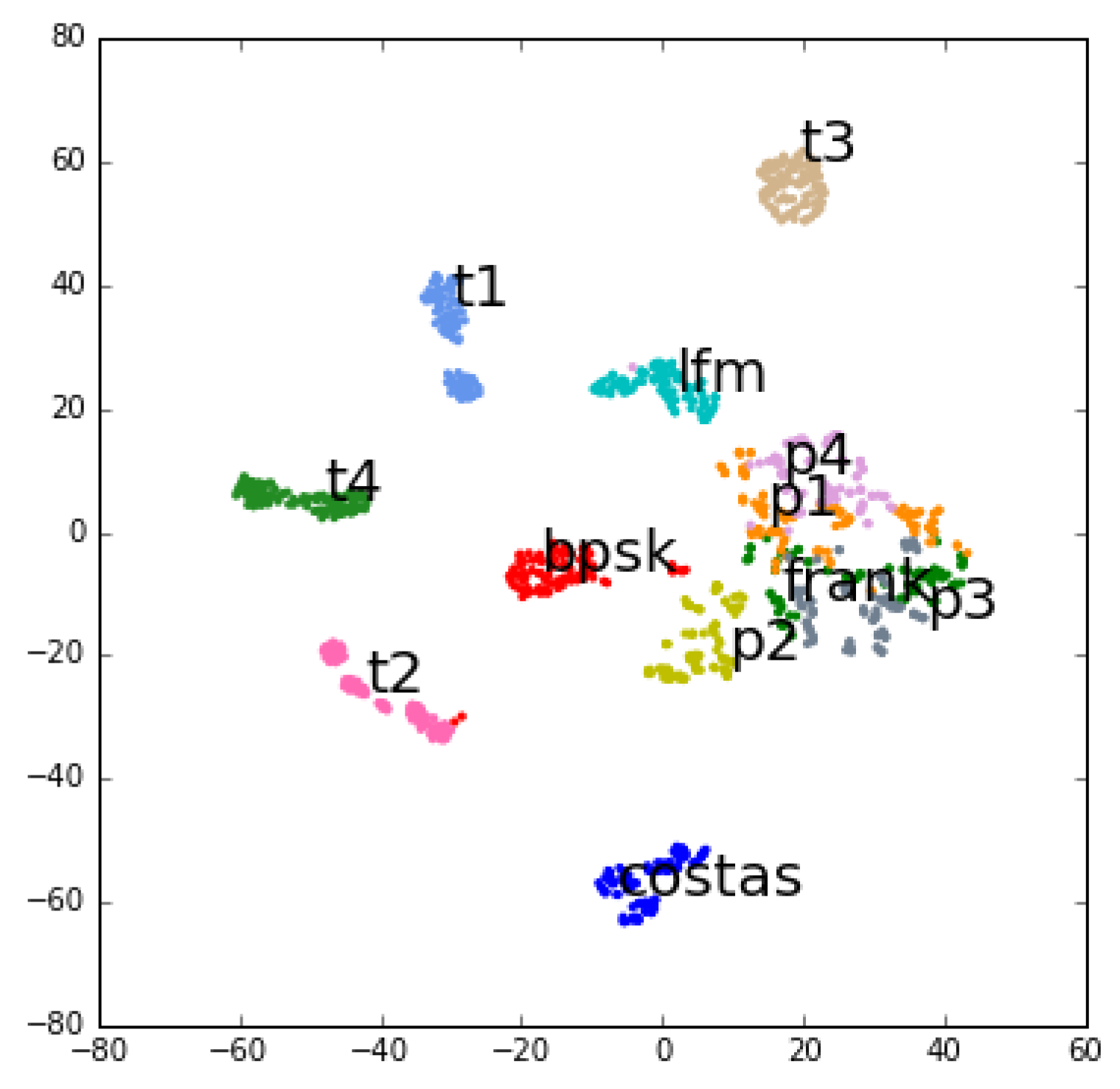
4.2. Feature Extraction

When the CNN model is trained, we choose a callback function to adjust the learning rate. The initial learning rate is set to 0.01, and the loss value is detected every 10 training cycles. If the loss value is not changing, the learning rate is reduced, the learning rate is set to the original 30%, and the learning rate is set to a minimum of 0.0001.

The CNN model is trained and then saved. In the feature extraction, we input the training set and the test set radar waveform into the trained CNN model, respectively, remove the last layer of the fully connected layer (output layer), and extract the F6 data as the radar waveform feature $(84\times 1)$. After the feature extraction is completed, the feature is preprocessed. First, the feature is normalized to $[0,1]$, and then the feature is reduced by the PCA dimensionality reduction algorithm [21]. Finally, the dataset is sent to the TPOT optimized classifier for training and recognition. Normalization and dimensionality reduction can effectively reduce the complexity of classifier optimization.

5. TPOT Optimization Classifier

The system uses a tree structure-based process optimization tool (TPOT) to select and optimize classifier parameters. The tool uses a model of genetic programming (GP) [22] to automatically design and optimize machine learning processes. This section combines the characteristics of LPI radar waveform recognition problem with the advantages of machine learning process optimization, introduces the tool into the research of radar waveform recognition, and reduces the process complexity while ensuring the classification accuracy through the corresponding setting of genetic programming.

5.1. Genetic Programming

The basic idea of genetic programming draws on the principles of biological evolution and genetic theory in nature, and is a method for automatically generating search programs. As a new global optimization search algorithm, this algorithm is successfully applied to many different fields because it is simple, versatile, robust, and has strong ability to solve nonlinear complex problems. More in-depth research has been obtained in recent years.

To automatically select the classifier and optimize the classifier parameters, a genetic programming approach is used. The implementation uses a Python library called DEAP. In the case of this paper, the GP constructs a tree structure with process operation operators as nodes to maximize the final classification accuracy of the process. All processes start from inputting feature data to the end of the classifier, and the intermediate classifier is arbitrarily selected.

The GP algorithm follows a standard evolutionary algorithm program. Typical parameter settings are shown in

Table 2. Genetic programming parameter settings.

GP Parameter	Content
Population size	100
Number of iterations	10
Individual mutation rate	90%
Crossover rate	5%
Method of choosing	10% elite reserve, 3 choice 2 bidding selection method, according to complexity 2 choose 1
Mutation	Replace, insert, delete, each type of mutation each accounted for 1/3
Repeated operation	5

. At the beginning of each evolutionary process, the system randomly generates a fixed number of tree processes to form the primary population in genetic programming. These processes are then evaluated based on their classification accuracy, where the classification accuracy is the fitness of the individual processes.

After completing the evaluation of all process individuals, the system performs the next generation of the GP algorithm. To generate the next generation of the population, the system first creates a copy of the process individual with the highest fitness and places it in the population of the offspring until these elite individuals account for 10% of the total population (i.e., 10% of the elites retained strategy). To build the rest of the next generation’s population, the system randomly selects three individuals from the existing population and then puts them into tournaments to determine which individuals win. In this competition, the least-accommodating individuals are eliminated, and then the processes with lower process complexity (i.e., fewer operating nodes) are selected from the remaining two individuals, and their replication is placed in the next generation population. This selection process is repeated until the remaining 90% of the population is filled. After the creation of the next generation population, the system applies a point crossover operator to the replicated group of individuals selected by crossover rate. Each intersection will randomly select two individuals and divide at a random point in the process structure. The contents of each are then exchanged with each other, while the remaining unaffected individuals selected by mutation rate will be mutated.

• Replace mutation: The operational nodes in the individual process structure are randomly selected and replaced with new randomly generated process sequences.
• Insert mutation: A new randomly generated sequence of processes is inserted into the random location of the inserted individual.
• Remove mutation: A random culling sequence is performed on the processes of the deleted individual.

When a replicated individual is selected as a mutant individual, one third of each mutation operator acts on the mutant individual. Invalid processes are not allowed in all crossover and mutation operations. Invalid processes are not allowed in all crossover and mutation operations. For example, the process of passing a dataset to a node that is entered as a single parameter is not allowed.

After the crossover and mutation operations are completed, the previous generation of individuals is completely removed and the process of assessment-selection-crossover-variation is repeated with a fixed algebra. In this way, the GP algorithm continually changes the process, adds new operational nodes, improves fitness, and eliminates redundant or influential operational nodes. The single best performance process discovered by the system during evolution will be tracked and stored in a separate location, as the final optimization result of the process after the end of the run.

5.2. Classifier Model Selection and Optimization

Since the recognition object is basically a tagged data sample, the TPOT uses a supervised learning model, including tree structure based decision tree classifier (Decision Tree), random forest classifier (Random Forest) and Gradient Boosting, as well as support vector machine (SVM), logistic regression (Logistic Regression) and K-nearest neighbor method (KNN). For example, when SNR = −2 dB, the result of the TPOT optimized classifier is: Best pipeline: ExtraTreesClassifier (LogisticRegression (inputmatrix, C = 25.0, dual = True, penalty = l2), bootstrap = False, criterion=gini, max–features = 0.8, min–samples–leaf = 3, min–samples–split = 3, n–estimators = 100.

As can be seen from the above, TPOT selects Extra Trees Classifier as the classifier, where bootstrap is set to False, thus the whole dataset is used to build each tree. The function to measure the quality of a split is: criterion = “gini”. The number of features to consider when looking for the best split is: max–features = 0.8. The minimum number of samples required to be at a leaf node is: min–samples–leaf = 3. The minimum number of samples required to split an internal node is: min–samples–split = 3. The number of trees in the forest is: n–estimators = 100. Stacking Estimator is Logistic Regression. Inverse of regularization strength is: C = 25. The number used to specify the norm used in the penalization is: penalty = “12”.

6. Simulation Experiment

We verified the proposed recognition model with an experimental simulation of the optimization algorithm. All generated data were simulated in MATLAB 2016a. The software used in the radar waveform classification section was Spyder (Python 3.5), including pre-processing, CNN feature extractor design, and TPOT classifier selection and optimization.The specific simulation environment is shown in

Table 3. The testing environment.

Item	Model/Version
CPU	i5-8300H(Intel)
GPU	NVIDIA GeForce GTX 1050 Ti
Memory	16 GB(DDR4 @2667 MHZ)
MATLAB	R2018b
Spyder	Python 3.5

. The first part of this section gives the simulation parameters of the low intercept probability radar, the second part verifies the validity of the CNN extraction feature, the third part verifies the performance of the optimization algorithm, the fourth part identifies the success rate of the model, and the last part verifies the robustness of the system. Details are as follows.

6.1. Create Sample

We generated the required radar waveforms through experimental simulations. In addition, the signal-to-noise ratio of the signal was $10lo{g}_{10}\left({\sigma }_s^2\right)/\left({\sigma }_{ϵ}^2\right)$, where ${\sigma }_s^2$ and ${\sigma }_{ϵ}^2$ are the variances of the signal and the noise, respectively. The parameters of each signal are different. We used $U(·)$ to represent the normalized frequency. For example, if we assume a certain frequency $f_0=1000$ Hz and the sampling frequency $f_s=8000$ Hz, the normalized frequency is expressed as $f_0=U(f_0/f_s)=U(1/8)$. The number of Barker codes used for BPSK signal modulation was randomly selected among 7, 11 and 13. The center frequency ranged from U(1/8) to U(1/4). The cycles per phase code cpp and code periods number were in the ranges of [1, 5] and [100, 300], respectively. For LFM signals, the signal length was 500–1024, the initial frequency was set between U(1/16) and U(1/8), and the bandwidth $\Delta f$ was also set between U(1/16) and U(1/ 8). The frequency hopping number was set to 3–6 for Costas signal. The frequency hopping fundamental frequency ($f_{min}$) was set between U(1/24) and U(1/20). For example, when a frequency hopping signal was generated, the frequency hopping frequency was 4. Next, a random non-repetitive sequence was generated and the difference triangle was satisfied, such as 3, 2, 1, 4. At this time, the frequency of frequency hopping was 3$f_{min}$, 2$f_{min}$, $f_{min}$, 4$f_{min}$. For the multi-time code T1–T4 signal, the number of basic waveform segments was set within the interval [4, 6]. The length of each cycle was normalized within [0.07, 0.1]. For the Frank signal, the center frequency was a random value between U (1/16) and U (1/8). cpp was 1–5. The phase control parameter M was 4–8. For P1–P4 polyphase codes, the parameters were similar to Frank code. For more details, see

Table 4. Simulation parameter list [9].

Radar Waveform	Simulation Parameter	Ranges
	Sampling frequency $f_s$	1($f_s=8000$ HZ)
BPSK	Barker codes $N_c$	{7,11,13}
	Carrier frequency $f_c$	U(1/8,1/4)
	Cycles per phase code cpp	[1, 5]
	Number of code periods np	[100, 300]
LFM	Number of samples N	[500, 1024]
	Bandwidth $\Delta f$	U(1/16,1/8)
	Initial frequency $f_0$	U(1/16,1/8)
Costas	Fundamental frequency $f_{m}in$	U(1/24,1/20)
	Number change $N_c$	[3, 6]
	Number of samples N	[512, 1024]
Frank&P1	Carrier frequency $f_c$	U(1/8,1/4)
	Cycles per phase code cpp	[1, 5]
	Samples of frequency stem M	[4, 8]
P2	Carrier frequency $f_c$	U(1/8,1/4)
	Cycles per phase code cpp	[1, 5]
	Samples of frequency stem M	2 × [2, 4]
P3&P4	Carrier frequency $f_c$	U(1/8,1/4)
	Cycles per phase code cpp	[1, 5]
	Samples of frequency stem M	2 × [16, 35]
T1–T4	Number of segments k	[4, 6]
	Overall code duration T	[0.07, 0.1]

. The signal-to-noise ratio interval was −6 dB to 8 dB, and the step size was 2 dB. Each type of signal produced 600 sets of data under each signal to noise ratio condition, with 500 sets for training and 100 sets for testing.

6.2. CNN Feature Validity Experiment

The experiment mainly verified the feasibility and effectiveness of the feature extraction of the CNN model. Five hundred training samples and 100 test samples of 12 types of radar signal waveforms were used under signal-to-noise ratio SNR = 8 dB. The time–frequency image preprocessed by the training samples was sent to the CNN model for training. After the training was completed, the pre-processed test data were input into the CNN model to extract the F6 layer data features, and then the extracted feature vectors were reduced by the tsne algorithm. The results of processing are shown in Figure 6.

It can be seen in Figure 6 that the characteristics of each type of signal are significantly different, which is convenient for classifier training and recognition. Therefore, it is feasible to extract the features of CNN F6 layer for radar waveform recognition.

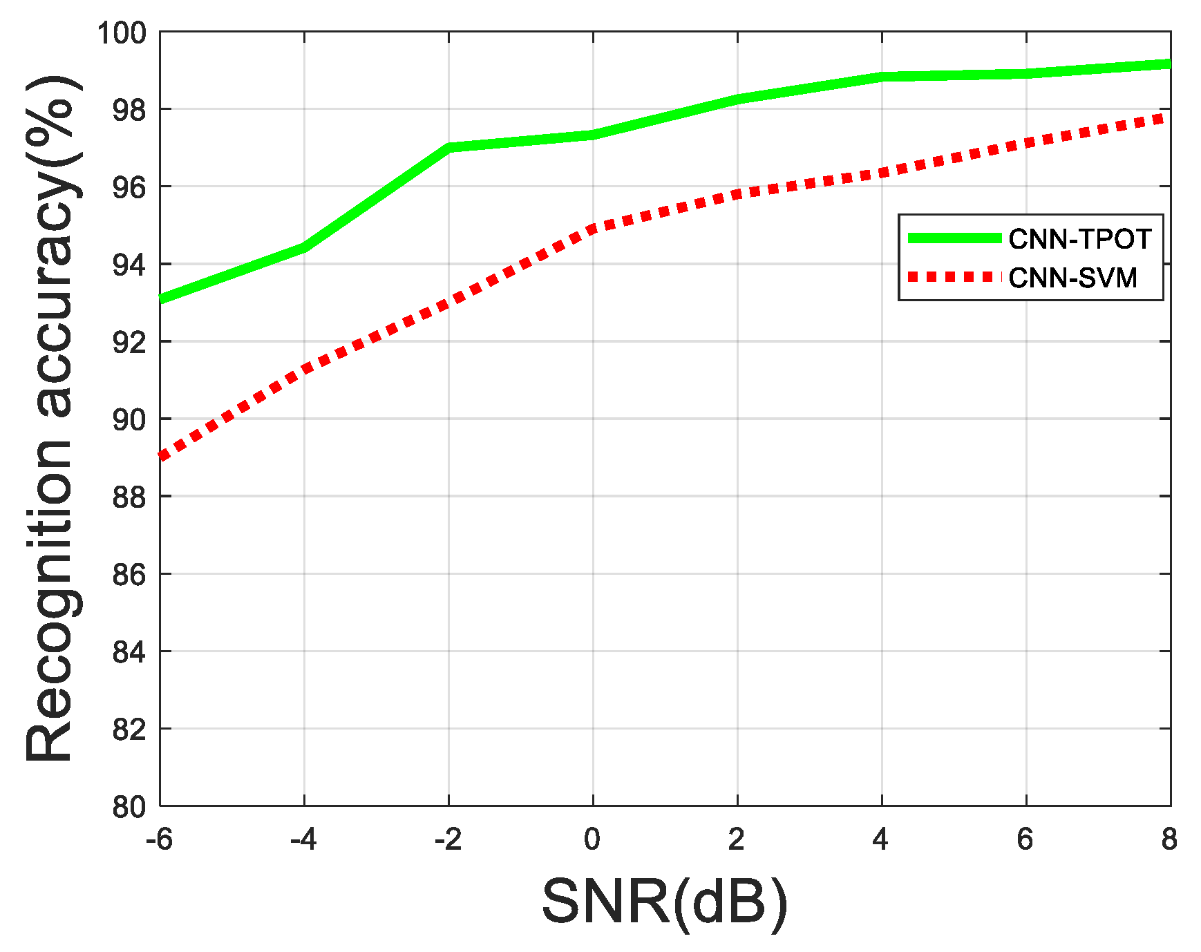
6.3. TPOT Optimized Classifier Performance Test

Next, we compared the accuracy of signal classification under different SNRs of TPOT and SVM [23], verified TPOT selection and optimized this superior classifier. The signal-to-noise ratio of the selected signal was increased from −6 dB to 8 dB, the length was 2 dB, and 600 sets of sample data were obtained for each signal-to-noise ratio, of which 500 were for training and 100 were for tests. The experimental results are shown in Figure 7.

As shown in Figure 8, as the SNR increased, the TPOT had a higher recognition rate, and, in the case of a large noise, the performance of the TPOT was significantly higher than that of the SVM. For example, at SNR = −6 dB, the recognition rate of TPOT was 3.17% higher than that of SVM. At SNR = −2 dB, the recognition rate of TPOT was 4% higher than that of SVM, and the growth rate was large, indicating that the TPOT selected and optimized classifier model has good anti-noise performance.

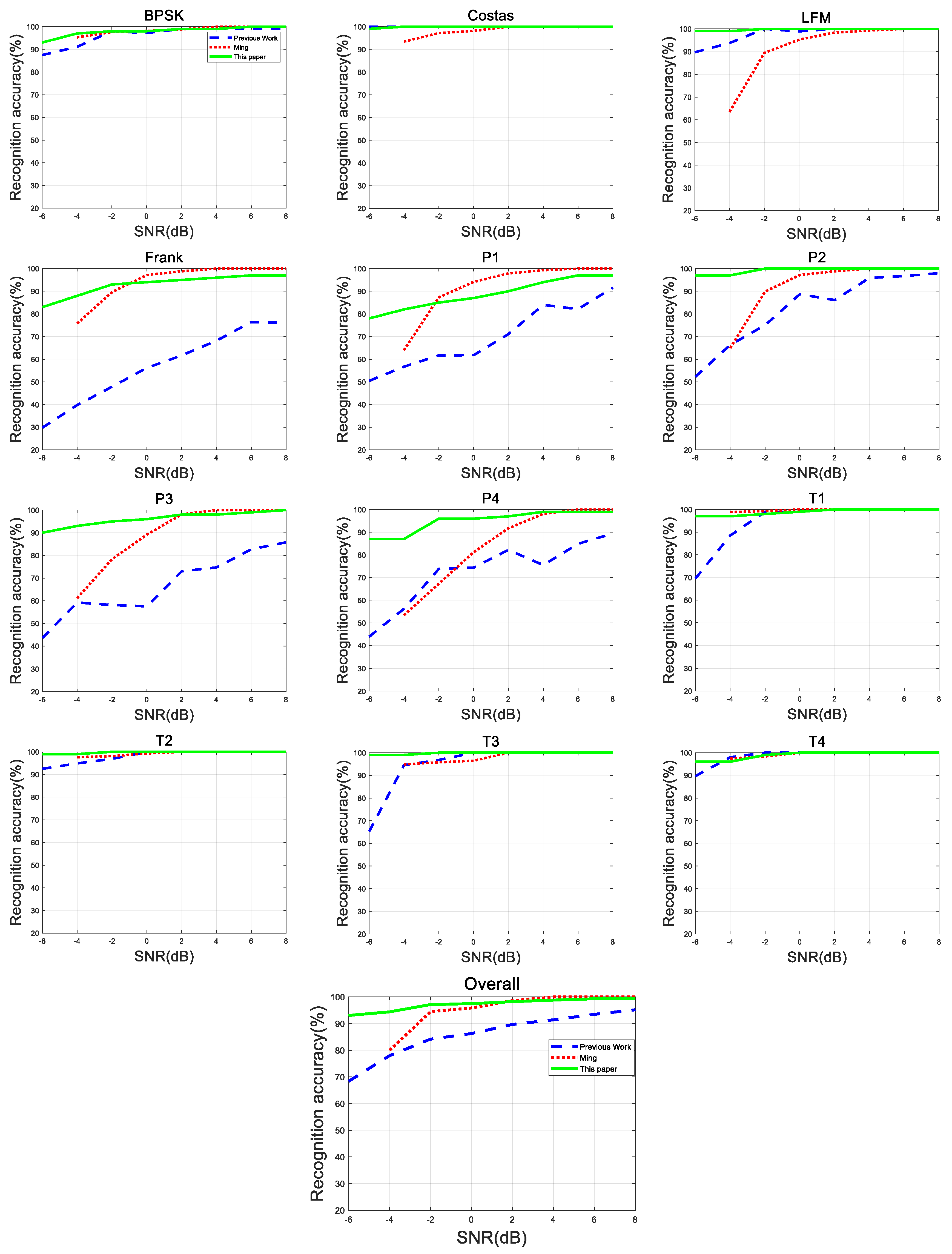
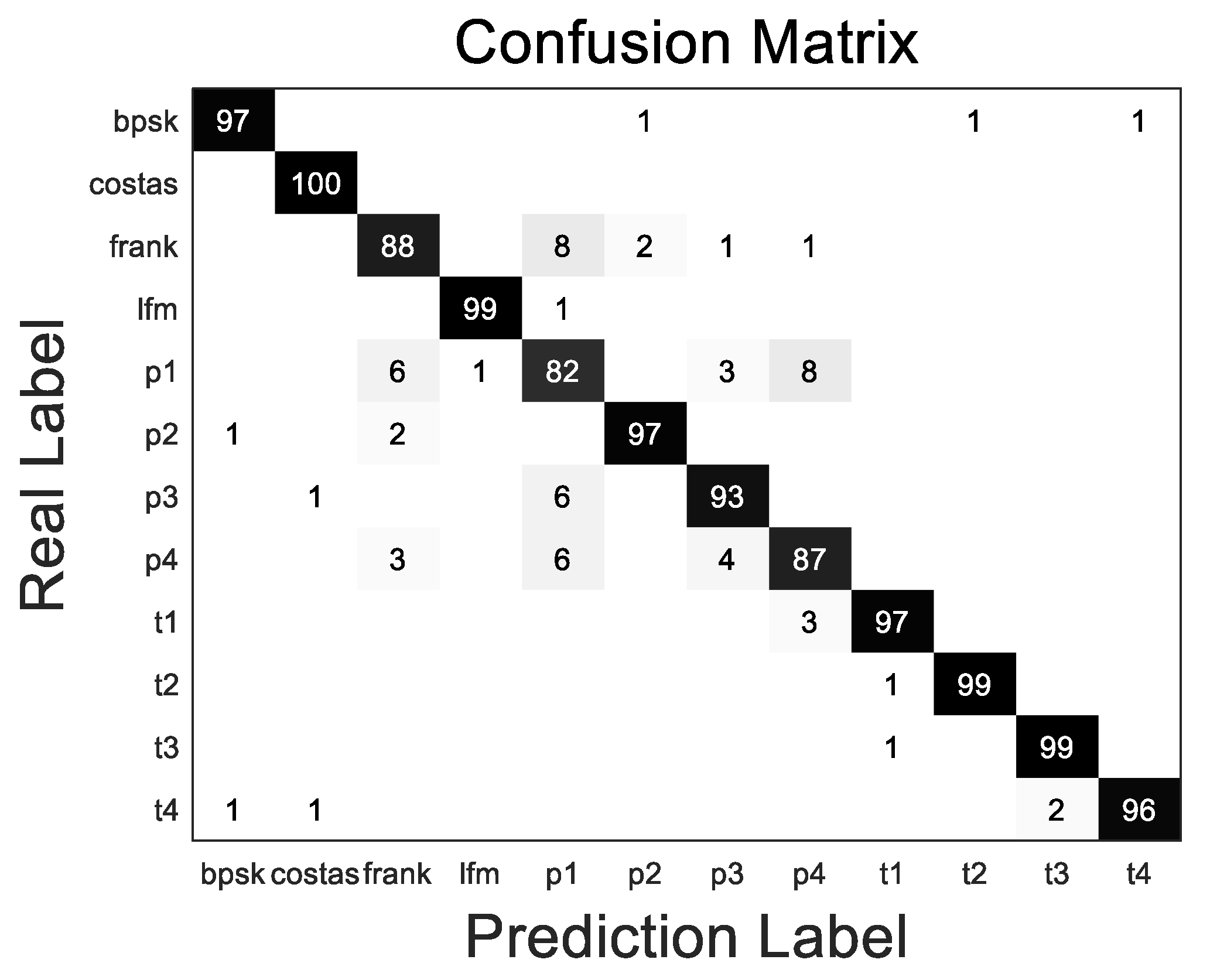
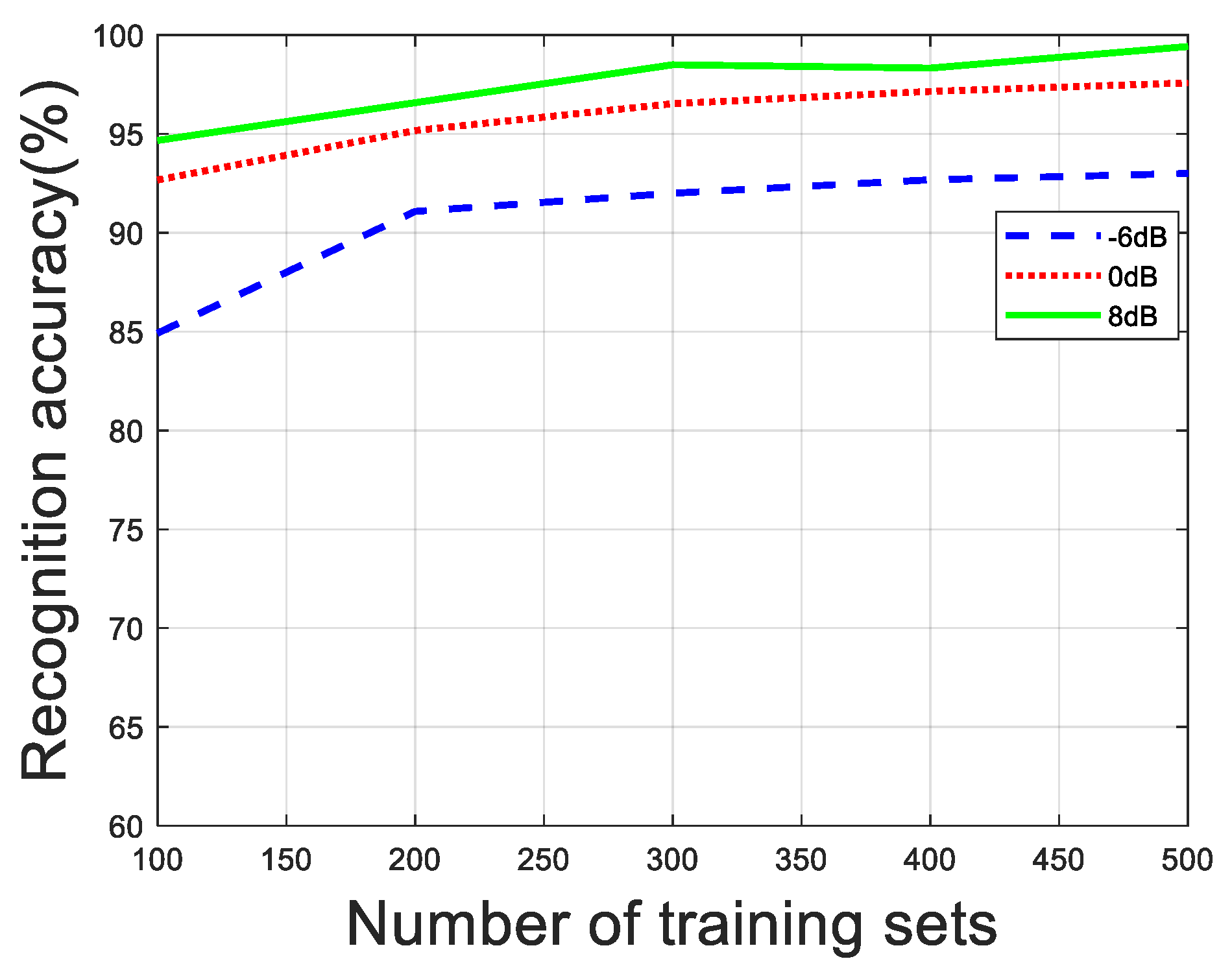
6.4. Experiment Results with SNR

The next experiment mainly verified the relationship between the recognition success rate and the signal-to-noise ratio. Five hundred groups of the sample dataset were used for offline training, and the remaining 100 groups were used for online testing. The signal-to-noise ratio of the signal was increased from −6 dB to 8 dB, and the length was 2 dB. This experiment compared the system of Ming [9] and our system, both of which are wide systems in waveform classification. The experimental results are shown in Figure 8.

It can be seen in the figure that, based on the identification system proposed in this paper, the recognition rate of 12 kinds of radar waveforms was proportional to the signal-to-noise ratio. With the increase of signal-to-noise ratio, the recognition accuracy of different types of radar waveforms gradually increased. When the signal-to-noise ratio was less than −2 dB, the recognition rate increased significantly. When the signal-to-noise ratio was greater than −2 dB, the recognition rate increased slowly and eventually stabilized. For LFM, the proposed method had better performance than the Ming method at low SNR, but it was not much different from our previous work. For polyphase codes (Frank and P1–P4) and multi-time codes (T1–T4), compared with Ming’s method, the recognition system had higher recognition rate under low SNR conditions. For example, when SNR = −4 dB, the recognition rate of the P2 signal was above 95%, and the recognition rate of the Ming method was less than 70%. When SNR = −4, the overall recognition rate of this system was 94.42%, Ming’s overall recognition rate was about 80%, and the previous algorithm recognition rate was 78%. It can be seen that this system had better performance under low signal-to-noise ratio. Our previous system only used the pre-training model to extract the time–frequency image features of the radar waveform, and did not use the radar waveform dataset to train the model. Therefore, the classification effect of the radar waveform (polyphase code) having a small difference from the time–frequency image pattern was poor. The system proposed in this paper used the radar waveform data training network. Thus, the system proposed in this paper was more accurate than the previous system. However, under high SNR conditions, the recognition accuracy of some radar waveforms was less than 100%. For example, at SNR = 6 dB, the recognition accuracy of the Frank, P1, and P4 radar waveforms did not reach 100%. Considering that radar signals are usually transmitted in complex environments with low SNR, it will be of great significance to have a good recognition effect under low SNR conditions.

Figure 9 is a confusion matrix diagram of 12 types of waveforms at SNR = −4 dB. It can be seen in the figure that, under low SNR conditions, signals with similar time–frequency images were easily confused. Taking P1 encoding as an example, the correct rate of the identification system proposed in this paper was 82%, 6% was misidentified as Frank code, 1% was misidentified as LFM code, 3% was misidentified as P3 code, and 8% was misidentified as P4 code.

6.5. Experiment with Robustness

The robustness test was to verify the reliability of the identification method under small sample conditions. For radar waveforms, it is impossible to build a large and complete experimental database as with other classification databases. Therefore, the system must have a good correct recognition rate under ultra-small sample conditions. In this experiment, each signal-to-noise ratio of 100 signals was used for testing, while the training samples were incremented from 100 to 500, with a length of 100. Experiments were repeated with −6 dB, 0 dB and 8 dB signal samples, respectively. The experimental results are shown in Figure 10.

As shown in Figure 10, as the training data increased, the overall recognition accuracy of the radar waveform gradually increased under the three signal-to-noise ratios. Under the condition of low SNR, the size of the training set had a great influence on the recognition accuracy. When the SNR was −6 dB, the recognition curve of the identification system proposed in this paper was basically stable with 200 groups, and the recognition rate reached about 91%. This shows that the system still had excellent classification performance under the condition that the training samples were few, which is of great significance for the recognition of radar waveforms.

7. Conclusions

This paper proposes a CNN–TPOT radar waveform automatic recognition system, which combines feature extraction and classifier into a framework, uses data to learn features, reduces the huge workload of manual extraction features, and improves the efficiency of feature extraction. TPOT can be used to select and optimize classifier parameters to improve recognition accuracy. With the help of image processing method, the system preprocesses the CWD time–frequency image of LPI radar signal. Through preprocessing operation, the time–frequency image difference between different signals is significantly enhanced, which not only eliminates the redundancy between related information, but also reduces the feature dimension. The method proposed in this paper not only solves the problem of manual feature extraction, but also preserves the features of time–frequency image of radar signal, which improves the recognition accuracy of LPI radar signal modulation under low signal-to-noise ratio. The experimental results show that the overall recognition accuracy of CNN–TPOT system is 94.42% when SNR = −4 dB. However, under high SNR conditions, the recognition accuracy of some signals is not ideal. According to radar waveform classification, the radiation source can be effectively detected, tracked and located. It has important application value for wireless communication and radar countermeasure system. However, there are many radar waveforms in the air at all times. This method is suitable for the classification of known radar waveform samples, but not for unknown radar signal waveforms. How to achieve the classification of unknown radar waveforms and improve the accuracy of waveform recognition under high SNR is the focus of our future work.

References

1. Chen, T.; Liu, L.; Huang, X. LPI Radar Waveform Recognition Based on Multi-Branch MWC Compressed Sampling Receiver. IEEE Access 2018, 6, 30342–30354. [Google Scholar] [CrossRef]
2. Kishore, T.R.; Rao, K.D. Automatic intrapulse modulation classification of advanced LPI radar waveforms. IEEE Trans. Aerosp. Electron. Syst. 2017, 53, 901–914. [Google Scholar] [CrossRef]
3. Dezfuli, A.A.; Shokouhm, A.; Oveis, A.H.; Norouzi, Y. Reduced complexity and near optimum detector for linear-frequency-modulated and phase-modulated LPI radar signals. IET Radar Sonar Navig. 2019, 13, 593–600. [Google Scholar] [CrossRef]
4. Jenn, D.C.; Pace, P.E.; Romero, R.A. An Antenna for a Mast-Mounted Low Probability of Intercept Continuous Wave Radar. J. Abbr. 2019, 61, 63–70. [Google Scholar]
5. Zilberman, E.R.; Pace, P.E. Autonomous time-frequency morphological feature extraction algorithm for LPI radar modulation classification. In Proceedings of the 2006 International Conference on Image Processing, Atlanta, GA, USA, 8–11 October 2006. [Google Scholar]
6. Ma, J.; Huang, G.; Zuo, W.; Wu, X.; Gao, J. Robust radar waveform recognition algorithm based on random projections and sparse classification. IET Radar Sonar Navig. 2013, 8, 290–296. [Google Scholar] [CrossRef]
7. Lunden, J.; Koivunen, V. Automatic radar waveform recognition. IEEE J. Sel. Top. Signal Process. 2007, 1, 124–136. [Google Scholar] [CrossRef]
8. Zhang, M.; Diao, M.; Guo, L. Convolutional Neural Networks for Automatic Cognitive Radio Waveform Recognition. IEEE Access 2017, 5, 11074–11082. [Google Scholar] [CrossRef]
9. Ming, Z.; Ming, D.; Lipeng, G.; Lutao, L. Neural Networks for Radar Waveform Recognition. Symmetry 2017, 9, 75. [Google Scholar] [CrossRef]
10. Lutao, L.; Shuang, W.; Zhongkai, Z. Radar Waveform Recognition Based on Time-Frequency Analysis and Artificial Bee Colony-Support Vector Machine. Electronics 2018, 7, 59. [Google Scholar] [Green Version]
11. Zhang, M.; Liu, L.; Diao, M. LPI Radar Waveform Recognition Based on Time-Frequency Distribution. Sensors 2017, 16, 1682. [Google Scholar] [CrossRef]
12. Xu, B.; Sun, L.; Xu, L.; Xu, G. Improvement of the Hilbert method via ESPRIT for detecting rotor fault in induction motors at low slip. IEEE Trans. Energy Convers. 2013, 28, 225–233. [Google Scholar]
13. Feng, Z.; Liang, M.; Chu, F. Recent advances in time Ű frequency analysis methods for machinery fault diagnosis: A review with application examples. Mech. Syst. Signal Process. 2013, 38, 165–205. [Google Scholar]
14. Hou, J.; Yan, X.P.; Li, P.; Hao, X.H. Adaptive time-frequency representation for weak chirp signals based on Duffing oscillator stopping oscillation system. Int. J. Adapt. Control Signal Process. 2018, 32, 777–791. [Google Scholar] [CrossRef]
15. Qu, Z.Y.; Mao, X.J.; Deng, Z.A. Radar Signal Intra-Pulse Modulation Recognition Based on Convolutional Neural Network. IEEE Access 2018, 6, 43874–43884. [Google Scholar] [CrossRef]
16. Ataie, R.; Zarandi, A.A.E.; Mehrabani, Y.S. An efficient inexact Full Adder cell design in CNFET technology with high-PSNR for image processing. Int. J. Electron. 2019, 106, 928–944. [Google Scholar] [CrossRef]
17. Zhang, A.J.; Yang, X.Z.; Jia, L.; Ai, J.Q.; Xia, J.F. SRAD-CNN for adaptive synthetic aperture radar image classification. Int. J. Remote Sens. 2019, 40, 3461–3485. [Google Scholar]
18. Li, Y.; Zeng, J.B.; Shan, S.G.; Chen, X.L. Occlusion Aware Facial Expression Recognition Using CNN With Attention Mechanism. IEEE Trans. Image Process. 2019, 28, 2439–2450. [Google Scholar] [CrossRef]
19. Baloglu, U.B.; Talo, M.; Yildirim, O.; Tan, R.S.; Acharya, U.R. Classification of myocardial infarction with multi-lead ECG signals and deep CNN. Pattern Recognit. Lett. 2019, 122, 23–30. [Google Scholar] [CrossRef]
20. Zeng, K.; Wang, Y.N.; Mao, J.X.; Liu, J.Y.; Peng, W.X.; Chen, N.K. A Local Metric for Defocus Blur Detection Based on CNN Feature Learning. IEEE Trans. Image Process. 2019, 28, 2107–2115. [Google Scholar] [CrossRef]
21. Zhang, G.W.; Tang, B.P.; Chen, Z. Operational modal parameter identification based on PCA-CWT. Measurement 2019, 139, 334–345. [Google Scholar] [CrossRef]
22. Yun, L.; Li, W.; Garg, A.; Maddila, S.; Gao, L.; Fan, Z.; Buragohain, P.; Wang, C.T. Maximization of extraction of Cadmium and Zinc during recycling of spent battery mix: An application of combined genetic programming and simulated annealing approach. J. Clean. Prod. 2019, 218, 130–140. [Google Scholar] [CrossRef]
23. Wang, B.; Tian, R.F. Judgement of critical state of water film rupture on corrugated plate wall based on SIFT feature selection algorithm and SVM classification method. Nucl. Eng. Des. 2019, 347, 132–139. [Google Scholar] [CrossRef]
Figure 1. The system components.
Symmetry 11 00725 g001
Figure 2. The CWD transformation results for different LPI radar waveforms, namely LFM, BPSK, Frank, Costas code, P1–P4 code, and T1–T4 code. It can be seen that the time–frequency image distributions of different waveforms are different.
Symmetry 11 00725 g002
Figure 3. ITaking P1 encoding as an example, when the signal-to-noise ratio is 0 dB, by the signal pre-processing flow, after binarization, the noise is effectively suppressed.
Symmetry 11 00725 g003
Figure 4. Forty binary images are selected randomly from the train/test sets of SNR = 0 dB. All eight kinds of waveforms are included in the figure.
Symmetry 11 00725 g004
Figure 5. CNN structure diagram. [8]
Symmetry 11 00725 g005
Figure 6. One hundred test samples of feature 2D plot at SNR = 8 dB.
Symmetry 11 00725 g006
Figure 7. LPI radar waveform recognition rate of CNN–TPOT and CNN–SVM under different SNR.
Symmetry 11 00725 g007
Figure 8. IRecognition rate of LPI radar waveform under different SNR.
Symmetry 11 00725 g008
Figure 9. Twelve types LPI radar waveform recognition results under −4 dB SNR.
Symmetry 11 00725 g009
Figure 10. LPI radar waveform recognition accuracy under different training data.
Symmetry 11 00725 g010