Dragonfly Algorithm with Opposition-Based Learning for Multilevel Thresholding Color Image Segmentation

Abstract

Multilevel thresholding is a very active research field in image segmentation, and has been successfully used in various applications. However, the computational time will increase exponentially as the number of thresholds increases, and for color images which contain more information this is even worse. To overcome the drawback while maintaining segmentation accuracy, a modified version of dragonfly algorithm (DA) with opposition-based learning (OBLDA) for color image segmentation is proposed in this paper. The opposition-based learning (OBL) strategy simultaneously considers the current solution and the opposite solution, which are symmetrical in the search space. With the introduction of OBL, the proposed algorithm has a faster convergence speed and more balanced exploration–exploitation compared with the original DA. In order to clearly demonstrate the outstanding performance of the OBLDA, the proposed method is compared with seven state-of-the-art meta-heuristic algorithms, through experiments on 10 test images. The optimal threshold values are calculated by the maximization of between-class variance and Kapur’s entropy. Meanwhile, some indicators, including peak signal to noise ratio (PSNR), feature similarity index (FSIM), structure similarity index (SSIM), the average fitness values, standard deviation (STD), and computation time are used as evaluation criteria in the experiments. The promising results reveal that proposed method has the advantages of high accuracy and remarkable stability. Wilcoxon’s rank sum test and Friedman test are also performed to verify the superiority of OBLDA in a statistical way. Furthermore, various satellite images are also included for robustness testing. In conclusion, the OBLDA algorithm is a feasible and effective method for multilevel thresholding color image segmentation.

1. Introduction

Image segmentation is a vital processing stage of object recognition and robotic vision. It can be also considered as a technique which partitions the components of an image into several distinct and disjoint regions, based on some features such as color or texture. More precisely, the interested objects or meaningful contours can be extracted conveniently [1]. In general, each of the pixels in the same region is homogeneous whereas the adjacent regions vary greatly [2]. The fundamental goal of image segmentation is to simplify or change the representation of the given image, making it easier for human visual observation and analysis. Nowadays, the image segmentation technique has already become a widespread application in various fields, and more intensive research is carried out continually [3].

In the last few years, a great variety of methods has been proposed for image segmentation, which can be summarized as four types, including region-based method, clustering-based method, graph-based method, and thresholding-based method [4,5,6]. The criterion of the region-based method is that the entire image is divided into lots of subregions continuously, and then the subregions with similar characteristics are merged to obtain objects [7]; the clustering-based method divides the image pixels into several sub-collections based on the similarity such as K-means and hierarchical clustering algorithm [8]; in the graph-based method, the global segmentation and local information processing can be combined together based on the good correspondence between image and graph theory features [9]; thresholding-based method which employs the image histogram, and classifies the image pixels into corresponding regions by comparing with threshold values [10]. The thresholding technique has become the most popular compared with the existing methods because of its high accuracy and simple implementation. It composes of bi-level and multilevel segmentation depending on the number of thresholds [11]. Bi-level segmentation means a given image should be segmented into two classes with respect to a single threshold value, namely, object and background. Nevertheless, it is difficult to select a preeminent threshold when the histogram of the image is multi-modal [12]. Hence, in order to improve the universality and practicability of the thresholding-based method, some scholars and researchers extend bi-level into multi-level thresholding. This is tantamount to saying that a given image will be subdivided into several non-overlapping classes according to multiple threshold values.

Numerous techniques based on respective criteria has been developed for getting appropriate thresholds during the last couple of decades. They can be divided into two different categories: global and local [13,14]. Otsu’s method and Kapur’s entropy which belong to the former are the most widely used [15]. Otsu proposed an available method which selects the optimal threshold values by maximizing between class variance of each segmented class in 1979 [16]. Kapur’s method was presented by J. N. Kapur et al. in 1985, which is used to classify image into multiple classes by comparing the entropy of histogram [17], and a higher entropy value indicates more homogeneous classes. However, the significant limitations among the available techniques are that the computational time increases with the number of thresholds increasing, and then image segmentation becomes too complicated for classic methods to obtain satisfying threshold values [18,19]. Therefore, further research is proceeding in the field of multilevel thresholding color image segmentation to enhance the performance of traditional methods.

The purpose of optimization is to find the optimal solutions which are more realistic and feasible for a specific problem under certain constraints [20]. The segmentation of each image can be regarded as a different single-objective optimization problem. More specifically, the objective functions which to be optimized are established based on specific criteria, such as Otsu’s method and Kapur’s entropy in this paper. The decision variables represent segmentation thresholds of an image. The current problem has two constraint conditions, firstly the gray level must be the integer, then its values should be between 0 and 255. Swarm intelligence (SI) algorithms inspired by nature with respective unique global and local searching strategies have been effectively applied to the optimization field [21]. What’s more, in order to reduce the time complexity of traditional thresholding methods and maintain accuracy effectively, many scholars are devoted to combining multilevel thresholding image segmentation with SI algorithms practically. Such as He and Huang proposed a modified firefly algorithm (MFA) based on the processing of mutual attraction and movement in the swarm for color image segmentation, using between-class variance, Kapur’s entropy, and minimum cross entropy techniques [21]. Khairuzzaman and Chaudhury presented the grey wolf optimizer (GWO) using the Otsu’s method and Kapur’s method for image segmentation, which is inspired from the social hierarchy and hunting behavior of grey wolves [22]. In addition, particle swarm optimization (PSO) [23], bacterial foraging optimization (BFO) [24], bat algorithm (BA) [25], whale optimization algorithm (WOA) [26], artificial bee colony (ABC) [27], and cuckoo search algorithm (CSA) [28] are also used extensively in multilevel thresholding segmentation.

Meta-heuristic algorithms have their own limitations which reduce the possibility of obtaining the global optimal values. So far a mass of strategies have been propounded to avoid these weaknesses. Opposition-based learning (OBL) is a more remarkable and general-purpose choice among them [29], in which the better ones are selected from current individuals and its opposite solutions through comparison [30]. With advantages in increasing population diversity and accelerating the convergence, it has increasingly extensive applications in various fields. The combination of krill herd algorithm and OBL can solve complex economic load dispatch problems [31]. Ewees et al. [32] successfully embedded the OBL in the grasshopper optimization algorithm and used this method to solve four engineering problems, namely, the welded beam design problem, the tension spring design problem, the three-bar truss design problem, and the pressure vessel design problem.

The dragonfly algorithm (DA) is a swarm-based algorithm which was proposed in 2015 by Mirjalili [33]. The main inspiration of the DA algorithm is two different behaviors of dragonflies, static and dynamic which are similar to the exploration and exploitation phases of meta-heuristic optimization. Exploration plays a vital role in the early stage to search for the unknown promising regions. Exploitation makes a significant effect in the later stage to get closer to an optimal solution [34]. The position of each dragonfly in the search space denotes a solution in optimization process. The DA algorithm has been widely used in various fields, such as medical diagnosis [35], optimization of proportional-integral-derivative (PID) controller [36], and a benchmark study of brushless DC motor optimization [37]. Meanwhile the simulation results proved strong robustness and high accuracy of the DA algorithm.

It is evident that color images contain more information compared with common images, highlighting the difficulty of satellite image segmentation. Furthermore, there are some drawbacks of the standard DA algorithm mentioned as follows: premature convergence, unbalanced exploration -exploitation [38,39,40]. In order to enhance the performance of traditional DA algorithm to a certain extent, as well as provide an efficient method to solve the problems in multilevel thresholding image segmentation, a modified dragonfly algorithm combined with opposition-based learning (OBLDA) is presented in this paper. The advantages of the proposed method include powerful optimizing ability, higher precision, strong robustness and remarkable stability. In this paper, between-class variance and Kapur’s entropy are used as objective functions which will be maximized to find the optimal thresholds. The performance of the proposed method is evaluated using five satellite images and five natural images. Meanwhile, several state-of-the-art meta-heuristic algorithms are selected for comparison, such as DA [39], PSO [23], the sine cosine algorithm (SCA) [41], the BA [25], the harmony search algorithm (HSO) [42], ant lion optimization (ALO) [43], and the salp swarm algorithm (SSA) [44]. Furthermore, some indicators such as the peak signal to noise ratio (PSNR), the feature similarity index (FSIM), the structure similarity index (SSIM), the average fitness values, standard deviation (STD), and computation time are chosen as quality metrics to compare the performance of proposed algorithm with other algorithms. Wilcoxon’s rank sum test [45] and Friedman test [46] is also performed to verify the superiority of OBLDA in a statistical way.

The remainder of this paper is organized as follows: Section 2 introduces the needed dataset. Section 3 firstly introduces thresholding technique including between-class variance and Kapur’s entropy, then gives an overview of the standard dragonfly algorithm, and finally describes the proposed method based on opposition-based learning. Section 4 presents a description of experiment in detail. Subsequently, the experimental results of proposed algorithm compared to other algorithms and its analysis are discussed in Section 5. Finally, the conclusion is illustrated in Section 6.

2. Dataset

In this paper, the proposed algorithm is tested on ten standard test color images, namely Image 1, Image 2, Image 3, Image 4, Image 5, Image 6, Image 7, Image 8, Image 9, and Image 10, respectively. Images 1–5 are taken from the database of Berkeley University [47], which are of size 481 × 321, and satellite Images 6–10 are taken from [48], which are also of size 481 × 321. Besides, all the test images and their corresponding histogram images are presented in

Table 1. Original test images and the corresponding histograms.

Original Image	Histogram	Original Image	Histogram
Cow		Cat
Image 1		Image 2
Zebra		Weasel
Image 3		Image 4
Massif		The stark transitions and vertical ecology of the canyon.
Image 5		Image 6
Chesapeake Bay in America.		An area about 50 kilometers southeast of Paso de Indios.
Image 7		Image 8
The emergence of performance made by the Kilauea eruption.		The growth in the city of New Delhi and its adjacent areas.
Image 9		Image 10

.

3. The Proposed Method for Multilevel Thresholding

In this section, firstly, we introduce two most widely used image thresholding techniques, including Otsu’s method which is based on between class variance and Kapur’s method which is based on the criterion of entropy. Then, we present a brief description of the standard dragonfly algorithm. In the end, we describe the proposed method based on opposition-based learning, and it can be effectively applied to the initialization stage and updated stage.

3.1. Thresholding Technique

3.1.1. Otsu’s Method

The Otsu method selects the optimum values of thresholds for multilevel thresholding by maximizing between class variance of each segmented class [49]. It can be defined as follows: assume that $L$ denotes the number of gray levels in a given image so that the range of intensity values is $\left[0,L-1\right]$.

Otsu’s method also can be effectively used for multilevel thresholding problems. Assume that the given image is subdivided into $n$ classes so that there are $n-1$ optimal thresholds, through maximization of the objective function.

The objective function based between-class variance is calculated by:

$${\sigma }_B^2\left(t\right)={\displaystyle \sum _{k=0}^{n-1}{P}_k}{\left({\mu }_k-\mu \right)}^2$$

(1)

where $P_k$ represents the cumulative probabilities of each class; μ_k is the mean level of each class. $\mu$ is the mean level of whole image.

The optimum thresholds $t^{*}\left(t_1,t_{2,}\cdots t_n\right)$ are obtained by maximizing the between-class variance objective function. A higher value of objective function refers to better quality of the segmented images.

3.1.2. Kapur’s Entropy

The Kapur’s method is used to determine the optimal thresholding values based on the maximization of entropy. It has attracted the interest of a lot of researchers because of its superior performance and been widely applied to solve image segmentation problems. The entropy of a given image represents the compactness and separateness among distinctive classes [50].

Kapur’s method can be used for multi-level thresholding, and it can obtain the $n$ optimal thresholds $\left(t_1,t_{2,}\cdots t_n\right)$ based on the Kapur’s entropy maximization:

$$f\left(t_1,t_2,\dots \dots ,t_n\right)=H_0+H_1\dots H_n$$

(2)

where $H_0,H_1,\cdots ,H_n$ represent the entropies of distinct classes.

However, the foremost restriction between Otsu’s and Kapur’s methods is that the computational time is increasing exponentially as the number of thresholds increases. Hence, it is time-consuming in practical terms for multilevel image segmentation applications. In order to overcome the above shortcomings, this paper presents a novel method based on the modified dragonfly algorithm to find the optimal thresholds. The purpose is to find the optimal thresholds accurately by maximizing the objective function in less processing time and maintaining segmentation accuracy.

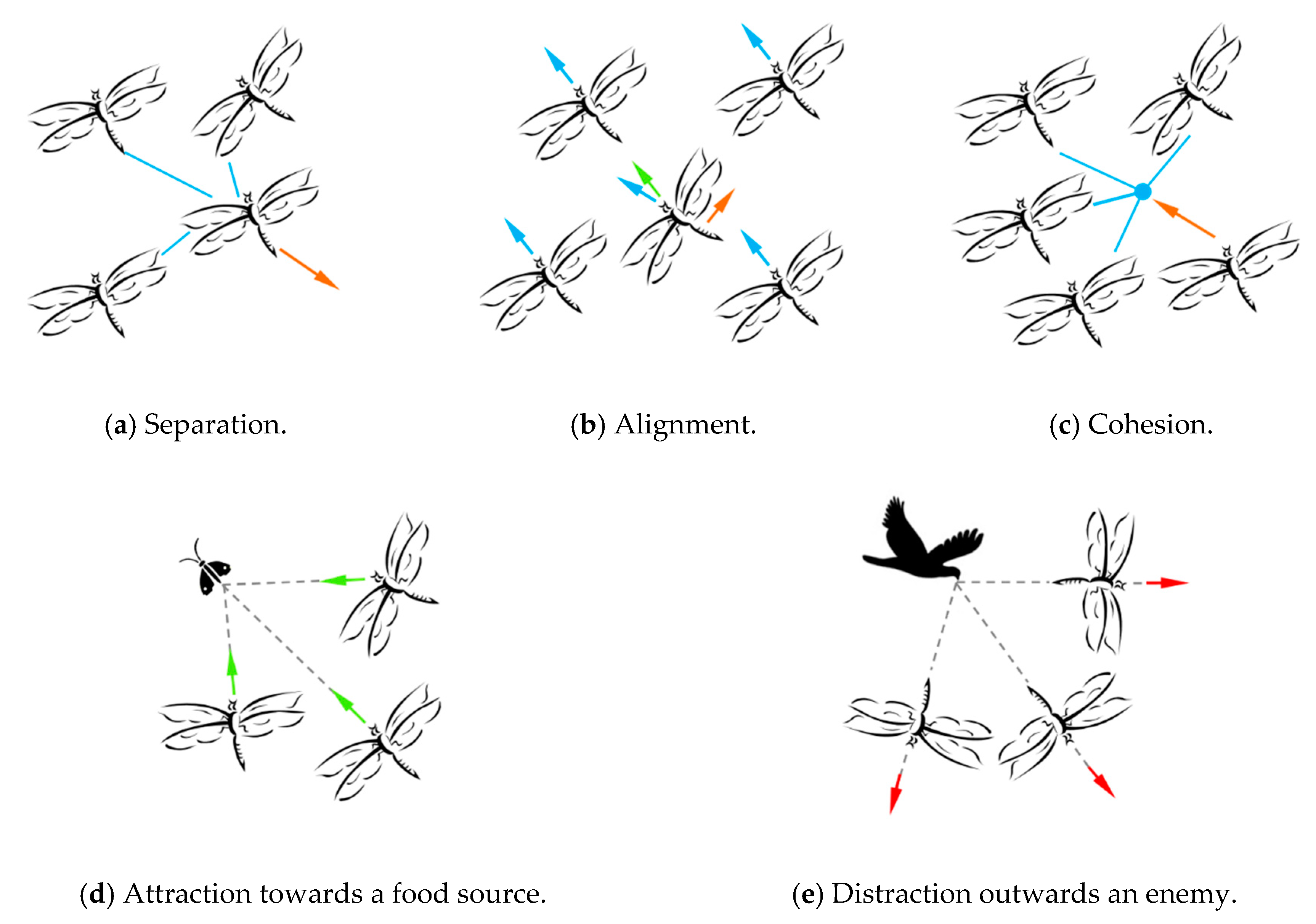
3.2. Dragonfly Algorithm (DA)

The dragonfly algorithm (DA) is a swarm-based algorithm which was proposed in 2015 by Mirjalili [33]. The main inspiration of the DA algorithm is two different swarming behaviors of dragonflies, static and dynamic. In static swarm, the dragonflies form several small groups which are characterized as local movements and abrupt changes in flying path, and afterwards they fly in all directions over a small area to search for food sources. Meanwhile in the dynamic swarm, a large number of the dragonflies fly in one direction with the purpose of migrating. Static and dynamic swarming behaviors are similar to the exploration and exploitation phases of meta-heuristic optimization. The position of each dragonfly in the search space denotes a solution in the optimization process.

Reynolds proposed that the behavior of swarms consists of three primitive principles, including separation, alignment, and cohesion These principles can be also adapted to the DA algorithm; besides, in order to model the swarming behavior of dragonflies in detail, two behaviors, the individuals of the swarm should be attracted towards food sources and diverted away from enemies, are also taken into account. Hence, the position of each dragonfly is updated by five different types of actions, which are mathematically modeled as Equations (3)–(7). Figure 1 shows primitive corrective patterns of dragonfly swarm. Meanwhile, in order to make a balance between exploration and exploitation, [33] defines $s,a,c,f,$ and $e$ as weight factors for separation, alignment, cohesion, attraction towards a food source, and distraction outwards by an enemy, respectively, which will adjust adaptively in DA algorithm. In addition, the two dragonflies are in the same neighborhood, in which the distance between them is less than the radius of neighborhood; on the contrary, they will be not in the same neighborhood. The radii of neighborhoods increases linearly with the number of iterations simultaneously to improve convergence speed, until all the dragonflies become one group at the final phase of optimization.

Separation:

$$S_i={\displaystyle \sum _{j=1}^W\left(X-X_j\right)}$$

(3)

where $X$ denotes the position of the current dragonfly. $X_j$ denotes the j-th position of neighboring dragonfly, and $W$ is the number of neighboring dragonflies.

Alignment:

$$A_i=\frac{{\displaystyle \sum _{j=1}^W{V}_j}}{W}$$

(4)

where $V_j$ is the velocity of the j-th neighboring dragonfly.

Cohesion:

$$C_i=\frac{{\displaystyle \sum _{j=1}^W{X}_j}}{W}-X$$

(5)

where $X$ represents the position of the current dragonfly. $X_j$ represents the j-th position neighboring dragonfly, and $W$ is the number of neighboring dragonflies.

Attraction towards a food source:

$$F_i=X^{+}-X$$

(6)

where $X$ shows the position of the current dragonfly, and $X^{+}$ shows the position of the food source, and it is chosen from the best dragonfly that the swarm has found up to now.

Distraction outwards by an enemy:

$$E_i=X^{-}+X$$

(7)

where $X$ denotes the position of the current dragonfly, $X^{-}$ denotes the position of the enemy, and it is chosen from the worst dragonfly that the swarm has found up to now.

The position of dragonfly is updated by:

$$X_{t+1}=X_t+\Delta X_{t+1}$$

(8)

where $\Delta X_{t+1}=\left(s{S}_i+a{A}_i+c{C}_i+f{F}_i+e{E}_i\right)+\omega \Delta X_t$, which can denote the direction of the movement.

When there is no neighboring individual, the behavior of dragonflies is assumed to be a random walk (Levy flight) around the search place to enhance randomness, stochastic behavior and exploration. The position of the dragonfly is updated as follows:

$$X_{t+1}=X_t+\mathrm{Levy}\left(d\right)\times X_t$$

(9)

where $t$ is the current iteration, and $d$ represents the dimension of position vectors.

Pseudo code of dragonfly for multilevel thresholding has been shown in Algorithm 1.

Algorithm 1. Pseudocode of dragonfly algorithm for multilevel thresholding

Initialize the position of dragonfly population $X_i\left(i=1,2,\dots ,n\right)$ based on opposition-based learning.

Initialize step vectors $\Delta X_i\left(i=1,2,\dots ,n\right)$.

WHILE the end condition is not satisfied

FOR $i=1:n$

Calculate the objective value of each dragonfly by using the Equation (1) for Kapur’s entropy or

Equation (2) for Between-class variance

Update the position of the food source $X_f$ and enemy $X_e$.

Update $w,s,a,c,f,$ and $e$

Calculate $S,A,C,F,$ and $E$ using Equations (4) to (7)

Update neighboring radius

IF a dragonfly has at least one neighboring dragonfly

Update velocity vector; Update position vector using Equation (8)

ELSE

Update position vector using Equation (9)

END IF

Select half of dragonflies from the current population randomly, and the opposition-based

learning is embedded in them.

Check and correct the new positions based on the boundaries of variables

END FOR

END WHILE

Return $X_f$, which represents the optimal values for multilevel thresholding segmentation.

3.3. Dragonfly Algorithm with Opposition-Based Learning (OBLDA) Based on Multilevel Thresholding

Opposition-based learning (OBL), which considers the current solution and opposite solution simultaneously to accelerate the convergence of meta-heuristic methods [30]. On the basis of probability theory, there is a 50–50 chance that the distance between the current solution and optimal solution is farther than its corresponding opposite [51]. Hence, we can utilize the concept of OBL to obtain a higher chance for approaching the promising regions, and then have a good balance of exploration and exploitation [52]. In general, the initial solutions are created randomly which are absence of priori knowledge about the solution. In addition, the convergence of the meta-heuristic methods will be time-consuming, when they are far away from the optimal solution. The applications of OBL can solve the problem in initialization effectively; meanwhile, the OBL also provides a strategy to search for the closer solution in the current population.

Let $x_{ij}^{}\left(x_{i1}^{},x_{2j}^{},\cdots ,x_{iD}^{}\right)$ be a point in D-dimensional space, and the opposite of $x_{ij}^{}$ is calculated by $x_{ij}^{\ast }\left(x_{i1}^{\ast },x_{i2}^{\ast },\cdots ,x_{iD}^{\ast }\right)$ as follow:

$$x_{ij}^{\ast }=k\left(a_j+b_j\right)-x_{ij}$$

(10)

where $a_j$ and $b_j$ are predefined as the lower and the upper bound of the search place respectively. $k$ represents the type of opposition-based learning.

The opposition-based learning can be employed in two stages of the standard DA effectively. Firstly, the OBL is embedded to the initialization of population to improve the diversity of dragonflies, and then the OBLDA algorithm can obtain fitter initial solutions which can help converge to global optimal solution accurately. Secondly, in the updating phase of the DA algorithm, the OBL is used in half of the current population randomly to check if the current solution is fitter than its corresponding opposite, increasing the randomness of the algorithm and saving more optimizing time simultaneously.

a. Initialization stage

The proposed method takes a random population $X$ of size $N$ as its initial solutions. $D$ is the number of dimension. The OBL is used to computed the opposite solution for each member. The steps of initialization are shown as follows:

Step 1: Initialize the population $X$ with a size of $N$ randomly.

$$x_{ij}=round\left(lb+\left(\left(ub-lb\right).\ast \left(rand\left(N,D\right)\right)\right)\right)$$

(11)

where, $ub$ and $lb$ are the upper and lower bound of search space.

Step 2: Calculate the opposite population $x_{ij}^{*}$ as:

$$x_{ij}^{\ast }=k\left(a_j+b_j\right)-x_{ij}; \left(i=1,2,\cdots ,N;j=1,2,\cdots ,D\right)$$

(12)

Step 3: Select a fitter one between $x_{ij}$ and $x_{ij}^{*}$ based on fitness function values to construct a new initial population.

b. Updated stage

In this stage, we select half of dragonflies from current population randomly which will be combined with the OBL, and then compute their fitness functions respectively based on the DA to choose the best solutions from $x_{ij}^{}\cup x_{ij}^{*}$. A new population will be generated using the OBLDA algorithm in each iteration. All the steps will be carried out constantly until the final conditions are reached.

Finally, the flowchart of OBLDA for finding the optimal threshold values is shown in Figure 2.

4. Experiments

In this section, firstly, we present a brief description of the experimental setup associated with multilevel thresholding. Then we show the parameter values which are used in all algorithms.

4.1. Experimental Setup

In this paper, two thresholding techniques namely Otsu’s method and Kapur’s entropy are used to determine the appropriate thresholds for color image segmentation. The performance of the proposed algorithm is compared with seven widely used optimization algorithms, namely the DA, PSO, SCA, BA, HSO, ALO, and SSA algorithms. All experiments are performed on ten test images with the following number of thresholds: 4, 6, 8, 10, and 12.

4.2. Parameter Setting

As we know, the value of parameters is of significance in determining the performance of each algorithm. In this paper, all algorithms have the same stopping conditions for a fair comparison. The max iteration is 500 with a total of 30 runs each algorithm, and the population size is set to be 30. The parameters of all algorithms are presented in

Table 2. Parameters of each algorithm.

Algorithm	Parameters Setting
DA [39]	Constant $\beta =0.5$
PSO [23]	Learning factors $c_1=c_2=2$, Maximum velocity $=25.5$
SCA [41]	Controlling parameter $r_1\in \left[0,2\right]$
BA [25]	Loudness $=0.25$; Factor updating pulse emission rate $\gamma =0.95$
HSO [42]	PAR (Pitch Adjustment Rate) $=0.3$ HMCR (Harmony Memory Considering Rate) $=0.95$
ALO [43]	controlling parameter $c_1\in \left[0,2\right]$
SSA [44]	Constant $\omega =\left[2.6\right]$

.

All the algorithms are developed by using “Matlab 2014b” and implemented on “Windows 10-64bit” environment on a computer having Pentium(R) Dual core T4500 @ 2.30 GHz and 2 GB of memory.

4.3. Segmented Image Quality Metrics

a. The peak signal-to-noise ratio (PSNR)

The parameter of PSNR based on the produced mean square error (MSE) is used to verify the difference of the original image and segmented image [53], and the value refers to the quality of the segmented image. The PSNR is evaluated by Equation (13).

$$PSNR=10{\log }_{10}\left(\frac{{255}^2}{MSE}\right)$$

(13)

where $I\left(i,j\right)$ and $K\left(i,j\right)$ are the original and segmented images which are of size $M\times N$.

b. The feature similarity index (FSIM)

A comparison of the features contained in the segmented image is performed using the FSIM and it is calculated as Equation (14). A higher FSIM value indicates a higher segmentation accuracy of the original image [54].

$$FSIM=\frac{{\displaystyle {\sum }_{x\in \Omega }{S}_L}\left(x\right)\times P{C}_m\left(x\right)}{{\displaystyle {\sum }_{x\in \Omega }P{C}_m\left(x\right)}}$$

(14)

where $\Omega$ represents the entire domain of the image. $P{C}_m\left(x\right)$ represents the phase congruence which is selected from the larger of the original and segmented images.

The value of $S_L\left(x\right)$ is defined as follows:

$$S_L\left(x\right)={\left[S_{PC}\left(x\right)\right]}^{\alpha }\cdot {\left[S_G\left(x\right)\right]}^{\beta }$$

(15)

where, $S_{PC}\left(x\right)$ is the similarity of phase consistency between two images. $S_G\left(x\right)$ is the similarity of gradient magnitude between two images.

c. The structure similarity index (SSIM)

The SSIM index, helps to access the structural similarity between the original and segmented image [55]. The value of SSIM index is in the range $\left[0, 1\right]$, and a higher value indicates better performance of algorithm. The value of SSIM equals 1 meaning that the two images are the same. The SSIM is defined as:

$$SSIM\left(x,y\right)=\frac{\left(2{\mu }_x{\mu }_y+c_1\right) \left(2{\sigma }_{xy}+c_2\right)}{\left({\mu }_x^2+{\mu }_y^2+c_1\right) \left({\sigma }_x^2+{\sigma }_y^2+c_2\right)}$$

(16)

where, ${\mu }_x$ and ${\mu }_y$ represent the average intensity of the original and segmented images respectively. ${\sigma }_x^2$ and ${\sigma }_y^2$ represent the variance of the original and segmented images respectively. ${\sigma }_{xy}$ is the covariance between the original and segmented images. $c_1$ and $c_2$ are constants.

5. Results and Discussions

In this section, we present the experimental results of the proposed algorithm compared to other algorithms based on Kapur’s entropy and Otsu’s method. The optimal threshold values for each of the color component as obtained by all algorithms and the segmented images can be found from [56]. The segmented results of natural images are show in Figure 3. Due to there being no absolute standard for a given image, we manually labeled the target region and separated it according to segmented results from the Berkeley dataset. And then took it as the ground truth for experimental comparison. It can be found from the figures that the targets obtained by the proposed method have been successfully separated from the complex background, which are similar to ground truth. Figure 4. shows the satellite segmented images with different threshold levels. We can observe from these figures, the images with higher level contains more detail than the others. The analysis in terms of PSNR, FSIM, SSIM, the average fitness function values and STD. A statistical analysis is also performed to see the advantage of the proposed algorithm outperforms all the other algorithms. All these are discussed in the following section.

5.1. Objective Function Measure

Between-class variance method and Kapur’s entropy are used as the objective functions that are maximized based on OBLDA, DA, PSO, SCA, BA, HSO, ALO, and SSA. In this way, each solution is represented by a real value which shows the quality of a solution.

Table 3. The average fitness values using Otsu’s method and Kapur’s method in comparison with other algorithms.

Images	K	Otsu’s Method								Kapur’s Entropy
		OBLDA	DA	PSO	SCA	BA	HSO	ALO	SSA	OBLDA	DA	PSO	SCA	BA	HSO	ALO	SSA
Image 1	4	3953.7954	3953.7954	3953.7950	3948.8042	3953.6831	3953.3067	3953.7954	3953.7954	18.5002	18.5000	18.4897	18.4613	18.4166	18.4963	18.5004	18.5000
	6	4019.8423	4019.5048	4018.7985	4006.9266	4017.3416	4017.2234	4018.8162	4018.8103	24.0001	23.9799	23.9811	23.6436	23.8908	23.8975	23.9811	23.9812
	8	4048.9152	4048.8504	4043.3223	4024.1493	4037.8143	4045.3231	4048.8877	4048.9101	28.8948	28.8129	28.7723	27.9375	28.5409	28.7200	28.8752	28.8702
	10	4063.1978	4063.1284	4061.1137	4039.0225	4050.5883	4059.3896	4062.5624	4061.703	33.4351	33.3523	33.1358	32.1934	31.8645	33.1194	33.3902	33.3934
	12	4070.6228	4070.1573	4070.6001	4054.429	4046.507	4066.2912	4069.932	4068.7841	37.4560	37.4284	37.3461	34.7885	35.2101	37.2779	37.4413	37.4221
Image 2	4	3485.1247	3485.1199	3485.1147	3479.1374	3484.6777	3484.7292	3485.1247	3485.1247	19.1186	19.1186	19.1185	19.1085	19.1174	19.1166	19.1180	19.1186
	6	3569.7989	3569.7975	3569.7922	3553.9263	3562.3733	3569.7989	3569.7902	3569.7900	24.5049	24.5036	24.5045	24.3797	24.4700	24.4768	24.5040	24.5040
	8	3604.7775	3604.7703	3604.6050	3576.8452	3583.8077	3600.4796	3604.7761	3601.4317	29.2700	29.2643	29.2628	28.6983	28.8901	29.1724	29.2609	29.2626
	10	3622.8818	3622.4558	3620.6747	3597.7083	3583.8832	3618.0966	3622.6152	3622.5331	33.6123	33.5556	33.5548	32.2689	32.6558	33.4410	33.5631	33.5566
	12	3631.3102	3630.5562	3630.7006	3614.941	3612.3747	3626.1269	3630.062	3630.8461	37.5249	37.5245	37.5247	34.4781	35.1123	37.1587	37.4867	37.4748
Image 3	4	1632.9348	1632.9348	1632.9325	1629.3742	1632.8832	1632.5101	1632.9329	1632.9348	17.9080	17.9078	17.9080	17.8708	17.9068	17.8966	17.9080	17.9078
	6	1679.6273	1679.6224	1679.6217	1663.4943	1675.7384	1678.9156	1678.6165	1679.0983	23.0198	23.0113	23.0190	22.8565	22.9702	22.9593	23.0187	23.0159
	8	1699.6539	1699.6112	1696.9162	1677.6783	1694.3511	1697.2418	1699.6475	1699.3764	27.6599	27.6578	27.5934	26.8723	27.5156	27.5298	27.6759	27.6531
	10	1709.7547	1709.2274	1709.5613	1691.5336	1689.6933	1704.8673	1709.7315	1709.4691	31.9288	31.9280	31.8964	30.1086	30.4496	31.6635	31.9204	31.9034
	12	1715.2551	1714.8516	1712.1207	1700.6739	1700.4449	1709.738	1715.0877	1714.0964	35.7785	35.2063	35.7770	32.6783	32.7375	35.2639	35.7784	35.1769
Image 4	4	1319.9491	1319.9489	1319.9491	1315.3303	1318.9811	1319.5916	1319.9491	1319.9488	18.4918	18.4916	18.4912	18.4622	18.4872	18.4819	18.4918	18.4918
	6	1369.0221	1369.0213	1368.9969	1357.1484	1366.7841	1367.9945	1369.0211	1369.0126	23.6922	23.6914	23.6905	23.4468	23.6669	23.6125	23.6912	23.6905
	8	1390.0326	1390.0305	1387.4005	1374.3224	1389.2622	1387.4095	1389.1814	1388.5589	28.3095	28.3024	28.3067	27.9281	27.9847	28.2587	28.3063	28.3095
	10	1399.6458	1399.4009	1393.7362	1384.4908	1384.9509	1396.9234	1399.0229	1187.096	32.5892	32.5865	32.5866	31.5723	31.3348	32.2579	32.5867	32.5830
	12	1405.8609	1405.6402	1404.5624	1384.8868	1393.2781	1401.2297	1403.591	1404.5764	36.3739	36.3688	36.3520	35.5627	34.4852	35.9779	36.3635	36.3490
Image 5	4	2424.6317	2424.5708	2424.5708	2421.2203	2424.5139	2424.2945	2424.5708	2424.5708	18.7381	18.7380	18.7372	18.6731	18.7217	18.7326	18.7368	18.7381
	6	2487.0084	2480.7669	2482.092	2478.4116	2485.5045	2483.8617	2487.0064	2487.0084	24.0292	24.0291	24.0237	23.6952	23.9584	24.0064	24.0234	24.0273
	8	2512.4189	2512.3053	2510.9344	2483.7068	2501.1752	2507.5583	2512.0236	2509.5901	28.7437	28.7079	28.7114	27.7347	28.2776	28.5286	28.7435	28.5687
	10	2525.6094	2523.4752	2519.899	2501.6225	2509.8173	2520.1389	2525.2327	2523.6277	32.9891	32.9847	32.9252	30.6967	31.0099	32.6646	32.9300	32.9754
	12	2530.8468	2528.9949	2529.6907	2516.2091	2520.8127	2527.7053	2529.6778	2530.163	36.8054	36.8009	36.0273	34.6304	34.6947	36.4877	36.8046	36.7984
Image 6	4	1729.2257	1729.2257	1710.9382	1726.02	1728.9882	1728.7219	1729.2257	1729.2257	18.7778	18.7777	18.7778	18.7436	18.7745	18.7679	18.7769	18.7771
	6	1779.9929	1779.9572	1779.9568	1763.9461	1779.0967	1777.7373	1779.9756	1779.9854	24.3551	24.3548	24.3540	24.1236	24.3076	24.3070	24.3542	24.3547
	8	1803.9526	1802.8008	1795.0211	1784.771	1790.259	1799.7721	1802.807	1802.7834	29.3048	29.2998	29.3031	28.8361	28.7555	29.1911	29.3036	29.3047
	10	1815.0429	1814.9534	1811.5293	1790.7357	1801.2403	1810.245	1814.0664	1814.4409	33.8351	33.8267	33.8347	31.9216	32.8086	33.6537	33.8307	33.8329
	12	1821.8206	1820.4563	1820.6098	1808.1162	1811.6587	1815.7141	1820.9947	1820.3147	37.9567	37.9542	37.9549	35.9544	35.8609	37.7342	37.9491	37.9458
Image 7	4	1400.5487	1400.5411	1401.5411	1398.0046	1400.263	1399.7372	1400.5411	1400.5411	18.8176	18.8176	18.7891	18.7644	18.8076	18.8011	18.7891	18.8176
	6	1441.0137	1440.9204	1440.957	1434.6068	1439.9286	1438.5452	1441.0115	1441.0045	24.2838	24.2726	24.2829	24.1141	24.0625	24.2560	24.2830	24.2811
	8	1459.6243	1459.4003	1457.3171	1444.2693	1437.1488	1454.8626	1459.6151	1459.5502	29.2380	29.2294	29.2352	28.9236	28.6026	29.1200	29.2287	29.1742
	10	1469.8421	1469.7252	1469.5444	1454.5045	1456.5918	1466.0482	1469.7097	1468.6476	33.6991	33.3882	33.5775	32.1851	31.6970	33.4260	33.5922	33.5392
	12	1475.6342	1475.1504	1470.2697	1458.6954	1464.184	1472.219	1475.04	1472.8635	37.7112	37.7027	37.7076	36.0898	35.1335	37.5058	37.7066	37.7104
Image 8	4	1435.7222	1435.7222	1435.6897	1433.7968	1435.3505	1435.276	1435.7102	1435.7222	18.9585	18.9577	18.9585	18.9197	18.9482	18.9551	18.9583	18.9585
	6	1500.0958	1500.0244	1500.0858	1484.1328	1498.127	1497.5381	1500.0134	1500.0237	24.4135	24.4116	24.4134	24.2572	24.3735	24.3847	24.4119	24.4102
	8	1525.3523	1524.7003	1525.3076	1510.2877	1501.9411	1521.2577	1525.1779	1525.17	29.3185	29.3176	29.3148	28.8671	28.7157	29.2512	29.3110	29.3181
	10	1539.6603	1539.1758	1537.4876	1523.3336	1526.3035	1533.9908	1539.5515	1539.3363	33.7653	33.7651	33.7626	32.6958	31.8454	33.4981	33.7650	33.7640
	12	1547.4005	1547.3542	1542.4244	1530.2169	1535.4957	1542.9102	1547.3996	1547.319	37.8293	37.8240	37.8254	36.2574	35.9844	37.6199	37.8005	37.8229
Image 9	4	2853.1743	2853.1743	2853.1743	2849.576	2853.0584	2852.8073	2853.1743	2853.1743	18.7385	18.7381	18.7384	18.7146	18.7368	18.7333	18.7380	18.7399
	6	2915.6723	2915.6408	2894.6826	2890.4899	2905.9451	2914.0036	2915.6679	2915.6702	24.0631	24.0627	24.0627	23.7434	24.0047	23.9918	24.0582	24.0356
	8	2941.2851	2941.1941	2933.3113	2918.6224	2910.8135	2939.6153	2941.0111	2941.237	28.9499	28.9433	28.9440	28.1130	27.8489	28.7974	28.9490	28.9297
	10	2954.834	2954.2199	2951.2338	2927.0843	2937.4698	2950.6298	2954.8092	2954.7299	33.3109	33.3062	33.3021	31.6533	31.6872	33.3069	33.3070	33.2021
	12	2962.1541	2961.8913	2960.7891	2959.7651	2952.4187	2958.9889	2962.037	2961.0798	37.5425	37.5421	37.3316	34.9365	34.8915	37.3107	37.5144	37.4505
Image 10	4	1052.6908	1052.6841	1052.6714	1048.6873	1052.5839	1052.0294	1052.6908	1052.6908	18.8252	18.8252	18.8250	18.7850	18.8041	18.8167	18.8246	18.8246
	6	1098.1595	1098.1333	1092.3076	1074.308	1088.9246	1096.6478	1098.1543	1098.1595	24.4177	24.4173	24.4172	24.2592	24.3146	24.3716	24.4170	24.4144
	8	1119.4996	1119.4816	1113.553	1095.8843	1113.587	1118.2696	1119.4058	1119.4948	29.3734	29.3678	29.3727	28.5648	28.7556	29.2970	29.3724	29.3639
	10	1130.8408	1130.7943	1127.75	1112.7634	1119.2282	1126.4325	1130.8091	1130.5106	33.8442	33.8427	33.8357	32.6137	32.3177	33.7053	33.8423	33.8435
	12	1137.1022	1136.8308	1133.8866	1121.5446	1126.9476	1131.71	1137.0952	1136.4462	37.9201	37.9055	37.9185	37.9017	37.0123	37.5918	37.9171	37.9133

present the average fitness function values based multilevel thresholding after application of all algorithms, and the higher value of average fitness function indicates the better solution (bold is the best). As seen from the results, the proposed method obtained the highest value for almost all the cases when compared to DA, PSO, SCA, BA, HSO, ALO, and SSA. This indicates that the performance of the proposed algorithm is the most outstanding, it can improve segmentation accuracy while ensuring algorithm stability. For instance, the optimal fitness function values are 33.6991, 33.3882, 33.3775, 32.1851, 31.6970, 33.4260, 33.5922, and 33.4392 for OBLDA, DA, PSO, SCA, BA, HSO, ALO, and SSA, respectively, when Kapur’s method is applied on Image 7, the average fitness function value of the OBLDA algorithm is the highest and the ALO algorithm comes at the second rank followed by SSA, and the BA is the worst algorithm because of an exponentially varying pulse emission rate. The experiment results also shows that the proposed algorithm not only has the advantage of multidimensional function for extremum problems, but also shows strong engineering practicability in color segmentation.

5.2. Stability Analysis

Measure of how far a given variable is from the mean, which is used to evaluate stability. A lower value of STD indicates that the method is more stable. It is defined as follows:

$$STD=\sqrt{\frac{1}{n-1}{\displaystyle \sum _{i=1}^n{\left(f_i-\overline{f}\right)}^2}}$$

(17)

The lower the STD, the more stable the algorithm. Then the competitive results for 30 runs of OBLDA and other algorithms are shown in

Table 4. The standard deviation (STD) values using Otsu’s method in comparison with other algorithms.

Images	K	OBLDA	DA	PSO	SCA	BA	HSO	ALO	SSA
Image 1	4	0.000	0.134	0.013	5.200	0.165	0.276	0.000	0.000
	6	0.015	0.232	3.230	6.040	3.160	0.697	1.670	0.156
	8	0.189	0.340	3.780	5.150	7.220	1.090	1.470	1.710
	10	0.401	1.250	1.420	5.630	52.500	1.390	0.558	0.519
	12	0.431	0.579	0.685	4.620	4.690	0.986	0.625	0.805
Image 3	4	0.000	0.020	5.280	1.040	0.109	0.228	0.000	0.000
	6	0.067	0.090	3.410	4.890	7.150	0.690	0.070	0.074
	8	0.112	0.315	3.780	5.670	4.420	1.430	1.480	0.250
	10	0.199	2.310	1.860	3.650	4.480	1.460	0.503	0.588
	12	0.542	0.793	2.850	5.120	4.790	0.804	0.876	0.842
Image 5	4	0.004	0.024	4.150	5.630	4.500	0.492	0.026	0.000
	6	0.002	0.322	2.100	6.070	5.780	0.596	2.140	0.005
	8	0.012	1.580	1.450	2.560	9.090	1.210	1.010	0.058
	10	0.250	1.510	2.890	5.480	7.350	1.090	0.996	0.690
	12	0.610	1.080	2.100	3.350	5.210	1.170	0.744	0.881
Image 7	4	0.000	0.030	5.190	6.180	0.443	1.080	0.000	0.000
	6	0.003	0.178	2.360	4.890	3.550	0.480	0.007	0.006
	8	0.242	0.254	2.550	5.790	5.770	0.857	0.310	0.502
	10	0.398	0.460	1.020	2.450	4.780	1.370	0.394	0.489
	12	0.501	0.671	0.658	6.990	3.470	0.963	0.545	0.712
Image 9	4	0.000	0.000	0.278	1.100	0.105	0.370	0.002	0.000
	6	0.021	0.028	3.170	2.890	5.150	1.160	0.027	0.022
	8	0.196	0.216	3.630	3.460	5.190	0.660	0.199	0.201
	10	0.124	0.433	1.990	3.210	4.890	1.840	0.358	0.577
	12	0.232	0.272	1.310	2.660	3.990	0.892	0.993	1.180

and

Table 5. The STD values using Kapur’s method in comparison with other algorithms.

Images	K	OBLDA	DA	PSO	SCA	BA	HSO	ALO	SSA
Image 2	4	0.000	0.000	0.000	0.007	0.001	0.025	0.000	0.000
	6	0.000	0.000	0.000	0.031	0.051	0.033	0.000	0.001
	8	0.002	0.006	0.005	0.200	0.357	0.031	0.003	0.004
	10	0.015	0.073	0.305	0.313	0.478	0.033	0.015	0.059
	12	0.027	0.030	0.214	0.589	0.790	0.066	0.029	0.029
Image 4	4	0.000	0.000	0.001	0.015	0.001	0.021	0.001	0.000
	6	0.001	0.001	0.007	0.035	0.051	0.015	0.013	0.015
	8	0.021	0.021	0.028	0.251	0.313	0.064	0.022	0.030
	10	0.030	0.034	0.202	0.387	0.534	0.079	0.032	0.049
	12	0.039	0.043	0.467	0.508	0.602	0.055	0.048	0.060
Image 6	4	0.000	0.008	0.016	0.007	0.003	0.003	0.001	0.001
	6	0.002	0.004	0.003	0.034	0.024	0.012	0.001	0.001
	8	0.005	0.012	0.014	0.199	0.499	0.022	0.007	0.007
	10	0.012	0.033	0.012	0.266	0.742	0.035	0.035	0.027
	12	0.031	0.046	0.044	0.353	0.672	0.082	0.050	0.045
Image 8	4	0.000	0.000	0.000	0.008	0.012	0.003	0.001	0.000
	6	0.001	0.005	0.004	0.065	0.049	0.012	0.004	0.003
	8	0.002	0.019	0.002	0.185	0.201	0.037	0.012	0.002
	10	0.011	0.015	0.013	0.297	0.342	0.069	0.035	0.018
	12	0.022	0.033	0.026	0.355	0.426	0.033	0.048	0.027
Image 10	4	0.001	0.002	0.001	0.015	0.003	0.005	0.001	0.001
	6	0.002	0.002	0.002	0.057	0.053	0.022	0.002	0.002
	8	0.006	0.006	0.006	0.096	0.384	0.016	0.006	0.006
	10	0.001	0.017	0.006	0.232	0.498	0.051	0.003	0.010
	12	0.002	0.023	0.007	0.432	0.631	0.063	0.005	0.018

(bold is the best). From the whole results, it is found that the OBLDA algorithm obtained the lowest values in 46 out of 50 cases (Otsu’s method) and 47 out of 50 cases (Kapur’s entropy). Therefore, it is evident that the HHO-DE algorithm has more remarkable stability than other algorithms.

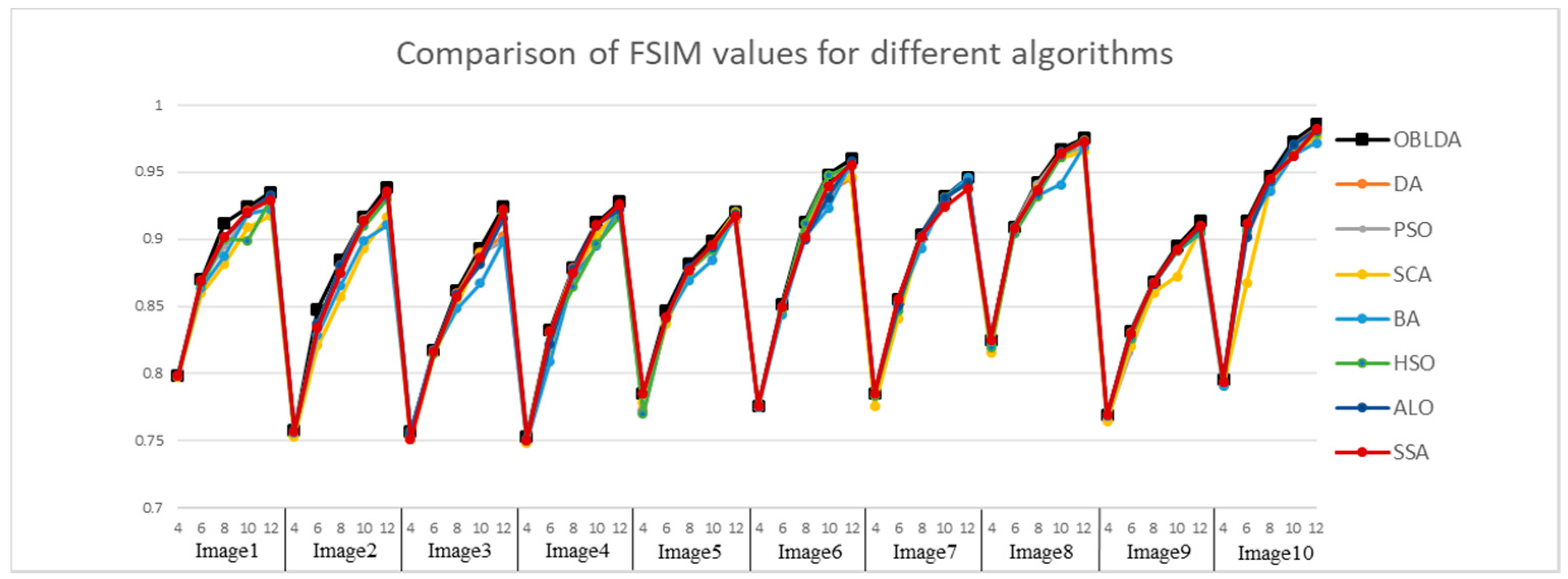
5.3. Segmentation Evaluation

In this section, we use PSNR, SSIM, and FSIM indicators to evaluate the segmentation accuracy of each algorithm. The higher the value of the indicator, the better the similarity with the original image (i.e., the higher segmentation quality). For a given image, if we take a limiting case into consideration, meaning there is no difference between original image and segmented image, the values of PSNR, FSIM, and SSIM are 1, 1, and infinity. Meanwhile, in order to easily and clearly observe in a way that is convenient for visual analysis, the line graphs of PSNR, SSIM, and FSIM are given in Figure 5, Figure 6, Figure 7, Figure 8, Figure 9 and Figure 10 respectively, From these figures it can be seen that, the black lines with square data points which represents the proposed method are located above other lines for the majority cases. Note that in order to make the structure more clear, we give the relevant experimental results in [56].

First of all, the PSNR index based on the grayscale information is used to estimate the degree of image distortion. The PSNR index values of the segmented images obtained by OBLDA, DA, PSO, SCA, BA, HSO, ALO, and SSA algorithm based on between-class variance and Kapur’s entropy are shown in Figure 5 and Figure 6. PSNR index gives a higher value when the degree of image distortion is small. A comparative analysis of the results indicates that the performance of all the algorithms was nearly close when K = 4, however, the proposed algorithm still show certain superiority over the other algorithms (such as Images 3 and 9). For instance, the PSNR values are 17.7278, 17.4278, 17.2685, 17.2833, 17.4849, 17.2554, 17.7270, and 17.7068 for OBLDA, DA, PSO, SCA, BA, HSO, ALO, and PSO, respectively, when the segmentation operation of Image 3 using Otsu’s method. The figures intuitively shows that as the number of thresholds increases, the PSNR values also increases for all algorithms, and the difference of value between the proposed method and other approaches is becoming more and more remarkable. It is evident that the proposed algorithm based on between-class variance or Kapur’s entropy for different threshold values is superior in performance to the other algorithms compared.

Then, the FSIM index based on phase consistency and spatial gradient feature is used to compare the quality of the segmented images and the range is [0, 1]. The FSIM values achieved using Kapur and Otsu method based OBLDA, DA, PSO, SCA, BA, HSO, ALO, and SSA are shown in Figure 7 and Figure 8. From the experimental results it is clearly observed that the proposed algorithm outperforms all the other algorithms for each benchmark image since the FSIM index in all cases obtains the highest values. Hence, the OBLDA algorithm using Kapur’s entropy and Otsu’s method has better quality for multilevel color image thresholding segmentation compared to other algorithms. For example, the FSIM index values in case of Image 10 with 10 thresholds based Kapur’s method are 0.9737, 0.9726, 0.9709, 0.9704, 0.9651, 0.9705, 0.9726, and 0.9731 for OBLDA, DA, PSO, SCA, BA, HSO, ALO, and PSO, respectively. It can be seen that the OBLDA came in the first rank and it has the highest FSIM values. The SSA algorithm is ranked second followed by ALO and DA, respectively. Due to PSO and SCA algorithm using linear decreasing inertia weight and control parameter to transform exploration and exploitation, they have no advantages in experiments. Through experimental results comparison and Figure 7 and Figure 8, it is no doubt that the FSIM value of the OBLDA associated with Kapur’s and Otsu’s method is largest and has the smallest gap with 1. The experiments also indicate that the proposed algorithm has high optimization accuracy and improves the segmentation quality.

After that, the SSIM index based on brightness, contrast and structural information is used to assess the visual similarity of the original image and the segmented image. The SSIM index values of the segmented images using Kapur’s entropy and Otsu methods obtained by all algorithms are given in Figure 9 and Figure 10. A higher value of SSIM index indicates that the segmented image is more similar to the original image. It can be seen from the results that, for the same image segmentation, the proposed algorithm achieves the best results which are more competitive in the SSIM values. At the same time, as the number of thresholds increases, the value of SSIM keeps increasing, and all algorithms can obtain more original image information Hence, we can extract the interested objects more accurately, and the segmented images is more similar to the original images visually. For example, the SSIM values of Image 2 using Otsu’s methods (OBLDA) are 0.6805, 0.7857, 0.8364, 0.8798, and 0.9031 for the number of thresholds is 4, 6, 8, 10, 12, respectively, as a contrast, the SSIM values of Image 2 using Otsu’s methods (DA) are 0.6775, 0.7754, 0.8354, 0.8788, and 0.9004 for the number of thresholds is 4, 6, 8, 10, and 12, respectively.

Through the above analysis, the proposed algorithm using Kapur’s method and Otsu’s method provide a great balance between exploitation and exploration in ten benchmark images at low and high threshold numbers. The performance of the OBLDA based multilevel thresholding for color image segmentation is satisfactory, for the reason that the segmented images has high quality and accuracy. It is evident the proposed algorithm can be effectively for solving color image segmentation problems.

5.4. Statistical Analysis

In this section, two well-established non-parametric tests are used to evaluate the significant difference between algorithms, meanwhile prove the improvement of OBLDA algorithm is remarkable in a statistical way, namely the Wilcoxon rand sum test [45] and Freidman test [46], respectively. The former is used for pairwise comparison and the latter for multiple comparison.

In the Wilcoxon rand sum test, the null hypothesis is defined as: there is no significant difference between the OBLDA algorithm and seven other algorithms. The alternative hypothesis considers a significant difference among them. The p-values are applicable to judge “whether or not to reject the null hypothesis”. If p-value is greater than 0.05 and h = 0 simultaneously, the null hypothesis will be rejected, indicating there is no significant difference among all algorithms. By contrast, the alternative hypothesis will be accepted at 5% significance level in which p is less than 0.05 or h = 1. The experiments are conducted 30 runs, and all obtained data are used for the testing.

Table 6. Statistical analysis of Wilcoxon rand sum test for the results.

Comparison	P-value (Otsu)	P-value (Kapur)
OBLDA versus DA	2.5389 × 10−6	5.1569 × 10−4
OBLDA versus PSO	1.4569 × 10−6	8.5902 × 10−5
OBLDA versus SCA	2.4901 × 10−8	3.7915 × 10−6
OBLDA versus BA	2.3762 × 10−4	6.8903 × 10−7
OBLDA versus HSO	6.3917 × 10−5	6.1372 × 10−5
OBLDA versus ALO	4.7835 × 10−6	1.0937 × 10−5
OBLDA versus SSA	0.1003	0.0005

shows the results of Wilcoxon rand sum test. It can be seen the table that P-values are much less than 0.05, both Otsu’s method and Kapur’s entropy. Therefore, there is a significant difference between OBLDA and other algorithms, in other words, the performance of proposed method has an remarkable improvement.

The null hypothesis $H_0$ in Friedman test states equality of medians between the algorithms, and the alternative hypothesis $H_1$ indicates the difference. The experimental results are shown in

Table 7. Statistical analysis of Friedman test for the results.

K	OBLDA	DA	PSO	SCA	BA	HSO	ALO	SSA	P-value
4	2.5167	3.7667	4.6333	7.3000	5.8333	6.0667	2.0833	3.3000	4.3904 × 10−23
6	1.5125	3.8625	7.2250	6.2000	5.3500	4.5125	3.5750	3.7625	2.1183 × 10−29
8	1.3534	3.8833	5.9000	5.9667	6.3500	5.2500	3.5333	4.1167	1.3943 × 10−20
10	1.0125	3.6375	4.8875	5.9375	6.7000	5.6625	3.7875	4.3750	2.9605 × 10−28
12	1.0125	4.5125	5.4250	6.0250	6.3125	5.1750	3.7250	3.8125	6.6435 × 10−26
all	1.2525	3.9450	5.1150	6.4250	6.3075	5.5350	3.6175	3.8025	1.3442 × 10−86

(bold is the best), including the average ranking of each algorithm at different threshold levels, the average overall ranking on all cases, and the P-value. It is observed that the proposed method obtains the best rank in the majority of cases. Meanwhile, the small P-value indicates the significant difference between the proposed method and others. Therefore, the promising results indicate that the performance of the OBLDA algorithm is improved markedly again. To sum up, the proposed method based on multilevel thresholding segmentation has superior performance compared with other algorithms.

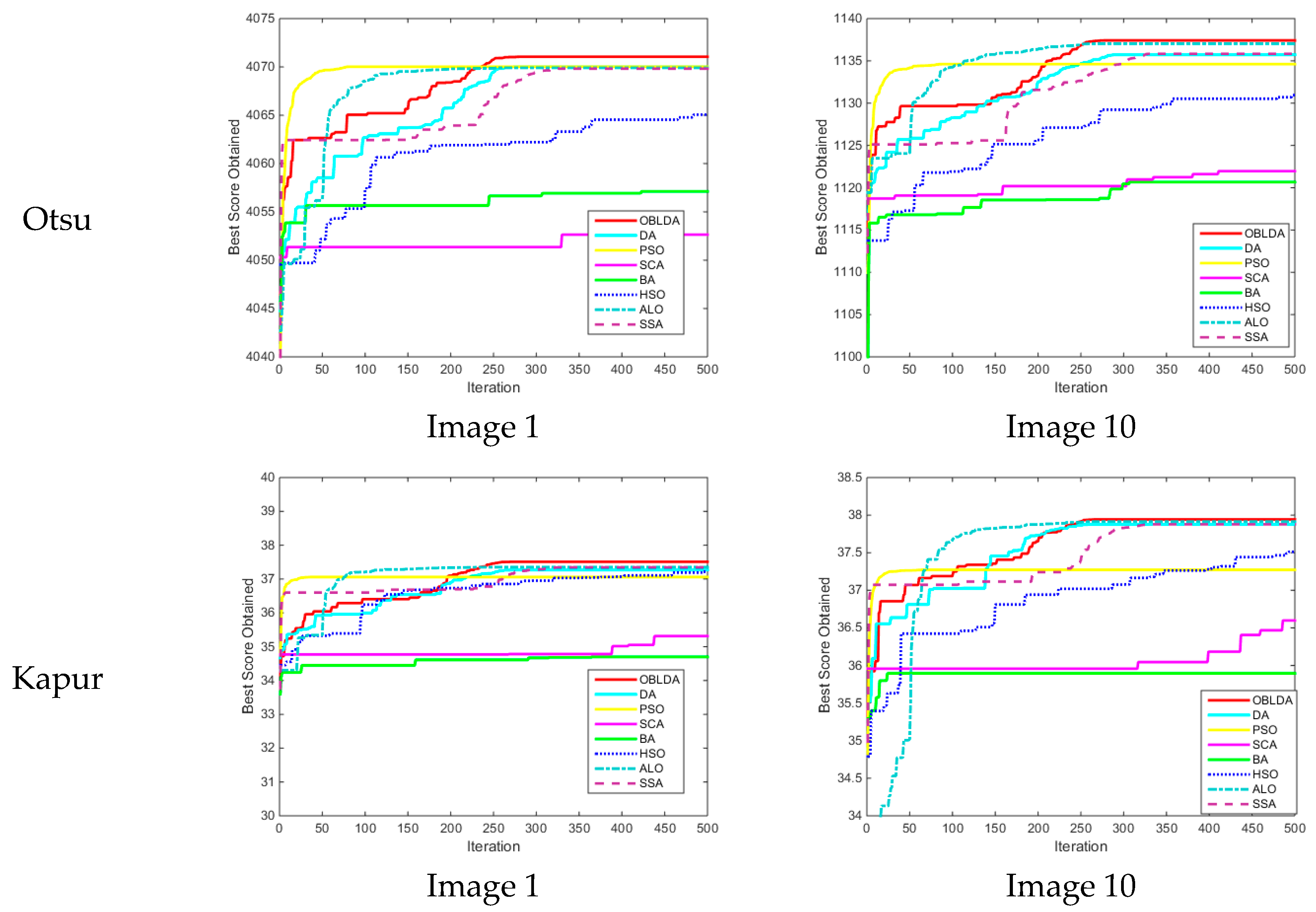
5.5. Convergence Performance

In this section, “Image 1” and “Image 10” are used for testing. The convergence curves of all algorithms using Otsu’s technique and Kapur’s entropy at 12 threshold levels are shown in Figure 11. From the figures, it is detected that the OBLDA algorithm has the most remarkable convergence property, and is capable of maintaining a good balance between exploratory and exploitative tendencies.

5.6. Computation Time

The average central processing unit (CPU) time of different algorithms considering all cases at 30 runs is given in

Table 8. The average time (s) considering all images under different threshold levels.

K	Exhaustive Search Method	Otsu’s Method			Kapur’s Method
		OBLDA	DA	Δ	OBLDA	DA	Δ
2	600.676	3.66784	3.78047	2.97%	3.76887	3.89403	3.34%
4	─	3.88478	4.10389	5.33%	3.87450	4.09988	5.37%
6	─	4.17290	4.46438	6.52%	4.13641	4.46217	7.39%
8	─	4.59074	4.99335	8.06%	4.58363	4.99469	8.21%
10	─	5.06321	5.52094	8.49%	5.04612	5.51358	8.52%
12	─	5.57285	6.20345	10.1%	5.56335	6.20046	10.3%

. It can be observed that the exhaustive search method takes a long time for optimization, but by contrast the DA and OBLDA algorithms obtain competitive results. When K = 2, the average time of exhaustive search method is already 600.676 s., which has grown to about 200 times DA or OBLDA algorithms. moreover, as the number of thresholds increases, the average time of each algorithm increases markedly, but the exhaustive search method behaves the fastest growth rates, which is far greater than DA and OBLDA algorithms. Then, it is seen that the OBLDA algorithm is slightly faster than DA, and can obtain the most appropriate threshold values. To sum up, the proposed method is significantly effective in color image multilevel thresholding.

5.7. Application in Plant Canopy Image

In this section, the OBLDA algorithm-based multilevel thresholding technique is applied to the field of plant canopy image segmentation. The purpose of this experiment is to verify whether the proposed method can solve segmentation problems in engineering practice. This section takes two plant canopy images as an example. Plant canopy is the first to be exposed to light and the external atmosphere, and it is closely related with plant growth. Hence, an accurate segmentation result of the plant canopy is vitally necessary for the assessment of plant growing state.

Figure 12 shows the original image, ground truth, and segmented image. It can be seen from the figures that the leaves have been successfully separated from the background, which are similar to the ground truth. Therefore, the proposed method can be used as a competitive technique to solve the segmentation problems in the plant canopy image.

6. Conclusions

The paper presents a novel multilevel thresholding technique based on the OBLDA algorithm for solving complex image segmentation problems. The opposite-based learning strategy can strengthen the diversity of population and avoid sinking into a local optimum during the optimization process. The between-class variance and Kapur’s entropy are used as objective functions, which are maximized to find the optimal threshold values. All experiments are performed on the five satellite images and five natural images, with the following number of thresholds: 4, 6, 8, 10, and 12. The performance of proposed algorithm is then compared with seven other algorithms. In addition, PSNR, FSIM, SSIM, the average fitness function values, computation time and STD are utilized as comparison metrics.

The results obtained indicate that most indicators showed a small difference in the case of K = 4, but the superiority of proposed algorithm becomes more and more remarkable as the number of thresholds increases. The competitive values of average fitness function, PSNR, FSIM, and SSIM prove the high accuracy of the OBLDA algorithm in the process of optimization. The significantly superior results of STD verify that the proposed method has a good stability. The Wilcoxon’s rank-sum test with 5% degree and Friedman test confirm the remarkable merits of the OBLDA algorithm compared to other algorithms in almost all cases. The promising results of computation time confirm the proposed method can converge to global optimal at a relatively rapid speed. The segmented results of plant canopy images is little different from groundtruth, and it can demonstrate the strong practicality of OBLDA algorithm in engineering. In addition, the OBLDA algorithm not only is effectively applied to Otsu’s method, but also has good adaptability in Kapur’s entropy. On the other hand, the proposed method shows excellent performance whether on satellite images or natural images, so it is provided with strong robustness. Hence, the proposed method can accomplish real-world and complex tasks of image segmentation effectively, as well as providing a more precise technique for multilevel segmentation.

In the future, we aim to find a much simpler and more effective method to strengthen the performance of the dragonfly algorithm for color image segmentation. We will also take up the deep study of how to make the proposed method adaptive to more practical engineering problems with superior performance.

References

1. Robert, M.; Carsten, M.; Olivier, E.; Jochen, P.; Noordhoek, N.J.; Aravinda, T.; Reddy, V.Y.; Chan, R.C.; Jürgen, W. Automatic segmentation of rotational X-ray images for anatomic intra-procedural surface generation in atrial fibrillation ablation procedures. IEEE Trans. Med. Imaging. 2010, 29, 260–272. [Google Scholar]
2. Qian, P.; Zhao, Y.; Jiang, K.; Deng, Z.; Wang, S.; Muzic, R.F. Knowledge-leveraged transfer fuzzy C-Means for texture image segmentation with self-adaptive cluster prototype matching. Knowl. Based Syst. 2017, 130, 33–50. [Google Scholar]
3. Lv, J.; Wang, F.; Xu, L.; Ma, Z.; Yang, B. A segmentation method of bagged green apple image. Sci. Hortic. 2019, 246, 411–417. [Google Scholar] [CrossRef]
4. Lee, S.H.; Koo, H.I.; Cho, N.I. Image segmentation algorithms based on the machine learning of features. Pattern Recognit. Lett. 2010, 31, 2325–2336. [Google Scholar] [CrossRef]
5. Breve, F. Interactive image segmentation using label propagation through complex networks. Expert Syst. Appl. 2019, 123, 18–33. [Google Scholar] [CrossRef] [Green Version]
6. Tang, N.; Zhou, F.; Gu, Z.; Zheng, H.; Yu, Z.; Zheng, B. Unsupervised pixel-wise classification for Chaetoceros image segmentation. Neurocomputing 2018, 318, 261–270. [Google Scholar] [CrossRef]
7. Meher, B.; Agrawal, S.; Panda, R.; Abraham, A. A survey on region based image fusion methods. Inf. Fusion 2019, 48, 119–132. [Google Scholar] [CrossRef]
8. Mittal, H.; Saraswat, M. An automatic nuclei segmentation method using intelligent gravitational search algorithm based superpixel clustering. Swarm Evol. Comput. 2019, 45, 15–32. [Google Scholar] [CrossRef]
9. Chen, J.; Zheng, H.; Lin, X.; Wu, Y.; Su, M. A novel image segmentation method based on fast density clustering algorithm. Eng. Appl. Artif. Intell. 2018, 73, 92–110. [Google Scholar] [CrossRef]
10. Ishak, A.B. A two-dimensional multilevel thresholding method for image segmentation. Appl. Soft Comput. 2017, 52, 306–322. [Google Scholar] [CrossRef]
11. Manikandan, S.; Ramar, K.; Iruthayarajan, M.W.; Srinivasagan, K.G. Multilevel thresholding for segmentation of medical brain images using real coded genetic algorithm. Measurement 2014, 47, 558–568. [Google Scholar] [CrossRef]
12. Fu, X.; Liu, T.; Xiong, Z.; Smaill, B.H.; Stiles, M.K.; Zhao, J. Segmentation of histological images and fibrosis identification with a convolutional neural network. Comput. Biol. Med. 2018, 98, 147–158. [Google Scholar] [CrossRef] [Green Version]
13. Li, J.; Tang, W.; Wang, J.; Zhang, X. A multilevel color image thresholding scheme based on minimum cross entropy and alternating direction method of multipliers. Optik 2019, 183, 30–37. [Google Scholar] [CrossRef]
14. Jiang, Y.; Tasi, P.; Yeh, W.; Cao, L. A honey-bee-mating based algorithm for multilevel image segmentation using Bayesian theorem. Appl. Soft Comput. 2017, 52, 1181–1190. [Google Scholar] [CrossRef]
15. Feng, Y.; Zhao, H.; Li, X.; Zhao, X.; Li, H. A multi-scale 3D Otsu thresholding algorithm for medical image segmentation. Dig. Signal Process. 2017, 60, 186–199. [Google Scholar] [CrossRef] [Green Version]
16. Otsu, N. A threshold selection method from gray-level histograms. IEEE Trans. Syst. Man Cybern. 1979, 9, 62–66. [Google Scholar] [CrossRef]
17. Kapura, J.N.; Sahoob, P.K.; Wongc, A.K.C. A new method for gray-level picture thresholding using the entropy of the histogram. Comput. Vis. Gr. Image Proc. 1985, 29, 273–285. [Google Scholar] [CrossRef]
18. Fredo, A.R.J.; Abilash, R.S.; Kumar, C.S. Segmentation and analysis of damages in composite images using multi-level threshold methods and geometrical features. Measurement 2017, 100, 270–278. [Google Scholar] [CrossRef]
19. Demirhan, A.; Törü, M.; Güler, İ. Segmentation of tumor and edema along with healthy tissues of brain using wavelets and neural networks. IEEE J. Biomed. Health Inf. 2015, 19, 1451–1458. [Google Scholar] [CrossRef] [PubMed]
20. Dirami, A.; Hammouche, K.; Diaf, M.; Siarry, P. Fast multilevel thresholding for image segmentation through a multiphase level set method. Signal Process. 2013, 93, 139–153. [Google Scholar] [CrossRef]
21. He, L.; Huang, S. Modified firefly algorithm based multilevel thresholding for color image segmentation. Neurocomputing 2017, 240, 152–174. [Google Scholar] [CrossRef]
22. Khairuzzaman, A.K.M.; Chaudhury, S. Multilevel thresholding using grey wolf optimizer for image segmentation. Expert Syst. Appl. 2017, 86, 64–76. [Google Scholar] [CrossRef]
23. Pham, T.X.; Siarry, P.; Oulhadj, H. Integrating fuzzy entropy clustering with an improved PSO for MRI brain image segmentation. Appl. Soft Comput. 2018, 65, 230–242. [Google Scholar] [CrossRef]
24. Pan, Y.; Xia, Y.; Zhou, T.; Fulham, M. Cell image segmentation using bacterial foraging optimization. Appl. Soft Comput. 2017, 58, 770–782. [Google Scholar] [CrossRef]
25. Ye, Z.; Wang, M.; Liu, W.; Chen, S. Fuzzy entropy based optimal thresholding using bat algorithm. Appl. Soft Comput. 2015, 31, 381–395. [Google Scholar] [CrossRef]
26. Aziz, M.A.E.; Ewees, A.A.; Hassanien, A.E. Whale Optimization Algorithm and Moth-Flame Optimization for multilevel thresholding image segmentation. Expert Syst. Appl. 2017, 83, 242–256. [Google Scholar] [CrossRef]
27. Gao, H.; Fu, Z.; Pun, C.; Hu, H.; Lan, R. A multi-level thresholding image segmentation based on an improved artificial bee colony algorithm. Comput. Electr. Eng. 2018, 70, 931–938. [Google Scholar] [CrossRef]
28. Pare, S.; Kumar, A.; Bajaj, V.; Singh, G.K. An efficient method for multilevel color image thresholding using cuckoo search algorithm based on minimum cross entropy. Appl. Soft Comput. 2017, 61, 570–592. [Google Scholar] [CrossRef]
29. Remli, M.A.; Mohamad, M.S.; Deris, S.; Samah, A.A. Cooperative enhanced scatter search with opposition-based learning schemes for parameter estimation in high dimensional kinetic models of biological systems. Expert Syst. Appl. 2019, 116, 131–146. [Google Scholar] [CrossRef]
30. Mahdavi, S.; Rahnamayan, S.; Deb, K. Opposition based learning: A literature review. Swarm Evol. Comput. 2018, 39, 1–23. [Google Scholar] [CrossRef]
31. Bulbul, S.M.A.; Pradhan, M.; Roy, P.K.; Pal, T. Opposition-based krill herd algorithm applied to economic load dispatch problem. Ain Shams Eng. J. 2018, 9, 423–440. [Google Scholar] [CrossRef]
32. Ewees, A.A.; Elaziz, M.A.; Houssein, E.H. Improved grasshopper optimization algorithm using opposition-based learning. Expert Syst. Appl. 2018, 112, 156–172. [Google Scholar] [CrossRef]
33. Seyedali, M. Dragonfly algorithm: a new meta-heuristic optimization technique for solving single-objective, discrete, and multi-objective problems. Neural Comput. Appl. 2016, 27, 1053–1073. [Google Scholar]
34. Shen, L.; Huang, X.; Fan, C. Double-group particle swarm optimization and its application in remote sensing image segmentation. Sensors 2018, 18, 1393. [Google Scholar] [CrossRef]
35. Díaz-Cortés, M.; Ortega-Sánchez, N.; Hinojosa, S.; Oliva, D.; Cuevas, E.; Rojas, R.; Demin, A. A multi-level thresholding method for breast thermograms analysis using Dragonfly algorithm. Infrared Phys. Technol. 2018, 93, 346–361. [Google Scholar] [CrossRef]
36. Guha, D.; Roy, P.K.; Banerjee, S. Optimal tuning of 3 degree-of-freedom proportional-integral-derivative controller for hybrid distributed power system using dragonfly algorithm. Comput. Electr. Eng. 2018, 72, 137–153. [Google Scholar] [CrossRef]
37. Kizhakkethil, S.R.; Murugan, S. Memory based hybrid dragonfly algorithm for numerical optimization problems. Expert Syst. Appl. 2017, 83, 63–77. [Google Scholar]
38. Sambandam, R.K.; Jayaraman, S. Self-adaptive dragonfly based optimal thresholding for multilevel segmentation of digital images. J. King Saud Univ.-Comput. Inf. Sci. 2018, 30, 449–461. [Google Scholar] [CrossRef] [Green Version]
39. Jafari, M.; Chaleshtari, M.H.B. Using dragonfly algorithm for optimization of orthotropic infinite plates with a quasi-triangular cut-out. Eur. J. Mech. A. Solids. 2017, 66, 1–14. [Google Scholar] [CrossRef]
40. Hariharan, M.; Sindhu, R.; Vijean, V.; Yazid, H.; Nadarajaw, T.; Yaacob, S.; Polat, K. Improved binary dragonfly optimization algorithm and wavelet packet based non-linear features for infant cry classification. Comput. Methods Programs Biomed. 2018, 155, 39–51. [Google Scholar] [CrossRef]
41. Mirjalili, S. SCA: A Sine Cosine Algorithm for solving optimization problems. Knowl.-Based Syst. 2016, 96, 120–133. [Google Scholar] [CrossRef]
42. Horng, M. A multilevel image thresholding using the honey bee mating optimization. Appl. Math. Comput. 2010, 215, 3302–3310. [Google Scholar] [CrossRef]
43. Moghaddam, M.J.H.; Nowdeh, S.A.; Bigdeli, M.; Azizian, D. A multi-objective optimal sizing and siting of distributed generation using ant lion optimization technique. Ain Shams Eng. J. 2018, 9, 2101–2109. [Google Scholar] [CrossRef]
44. Mirjalili, S.; Gandomi, A.H.; Mirjalili, S.Z.; Saremi, S.; Faris, H.; Mirjalili, S.M. Salp Swarm Algorithm: A bio-inspired optimizer for engineering design problems. Adv. Eng. Software 2017, 114, 163–191. [Google Scholar] [CrossRef]
45. Frank, W. Individual Comparisons of Grouped Data by Ranking Methods. J. Econ. Entomol. 1946, 39, 269–270. [Google Scholar]
46. Friedman, M. The use of ranks to avoid the assumption of normality implicit in the analysis of variance. J. Am. Stat. Assoc. 1937, 32, 676–701. [Google Scholar] [CrossRef]
47. The Berkeley Segmentation Dataset and Benchmark. Available online: https://www2.eecs.berkeley.edu/Research/Projects/CS/vision/grouping/segbench/ (accessed on 3 March 2019).
48. Landsat imagery courtesy of NASA Goddard Space Flight Center and U.S. Geological Survey. Available online: https://landsat.visibleearth.nasa.gov/index.php?&p=1 (accessed on 3 March 2019).
49. Jia, H.; Lang, C.; Oliva, D.; Song, W.; Peng, X. Hybrid Grasshopper Optimization Algorithm and Differential Evolution for Multilevel Satellite Image Segmentation. Remote Sens. 2019, 11, 1134. [Google Scholar] [CrossRef]
50. Bhandari, A.K.; Singh, V.K.; Kumar, A.; Singh, G.K. Cuckoo search algorithm and wind driven optimization based study of satellite image segmentation for multilevel thresholding using Kapur’s entropy. Expert Syst. Appl. 2014, 41, 3538–3560. [Google Scholar] [CrossRef]
51. Elaziz, M.A.; Oliva, D.; Xiong, S. An improved opposition-based sine cosine algorithm for global optimization. Expert Syst. Appl. 2017, 90, 484–500. [Google Scholar] [CrossRef]
52. Dinkar, S.K.; Deep, K. An efficient opposition based Lévy Flight Antlion optimizer for optimization problems. Int. J. Comput. Sci. Eng. 2018, 29, 119–141. [Google Scholar] [CrossRef]
53. Aldahdooh, A.; Masala, E.; Wallendael, G.V.; Barkowsky, M. Framework for reproducible objective video quality research with case study on PSNR implementations. Dig. Signal Process. 2018, 77, 195–206. [Google Scholar] [CrossRef] [Green Version]
54. John, J.; Nair, M.S.; Kumar, P.R.A.; Wilscy, M. A novel approach for detection and delineation of cell nuclei using feature similarity index measure. Biocybern. Biomed. Eng. 2016, 36, 76–88. [Google Scholar] [CrossRef]
55. Wang, Z.; Bovik, A.C.; Sheikh, H.R.; Simoncelli, E.P. Image quality assessment: from error visibility to structural similarity. IEEE T. Image Process. 2004, 13, 600–612. [Google Scholar] [CrossRef]
56. data-Dragonfly-Algorithm-with-Opposition-based-Learning-for-Multilevel-Thresholding-Color-Image-Segmentation. Available online: https://github.com/baoxiaoxue/Dragonfly-algorithm/blob/master/data-Dragonfly-Algorithm-with-Opposition-based-Learning-for-Multilevel-Thresholding-Color-Image-Segmentation.pdf (accessed on 8 March 2019).
Figure 1. Primitive corrective patterns of dragonfly swarm [33].
Symmetry 11 00716 g001
Figure 2. Framework of the dragonfly algorithm with opposition-based learning (OBLDA) based multilevel thresholding.
Symmetry 11 00716 g002
Figure 3. The segmented images of “Image 2”, “Image 3”, and “Image 4” using the threshold technique.
Symmetry 11 00716 g003
Figure 4. The segmented images of “Image 7”, “Image 8” and “Image 9” at 4, 8, and 12 threshold levels.
Symmetry 11 00716 g004
Figure 5. Comparison of PSNR values using Otsu’s method, at K = 4, 6, 8, 10, and 12.
Symmetry 11 00716 g005
Figure 6. Comparison of PSNR values using Kapur’s entropy, at K = 4, 6, 8, 10, and 12.
Symmetry 11 00716 g006
Figure 7. Comparison of feature similarity index (FSIM) values using Otsu’s method, at K = 4, 6, 8, 10, and 12.
Symmetry 11 00716 g007
Figure 8. Comparison of FSIM values using Kapur’s entropy, at K = 4, 6, 8, 10, and 12.
Symmetry 11 00716 g008
Figure 9. Comparison of SSIM values using Otsu’s method, at K = 4, 6, 8, 10, and 12.
Symmetry 11 00716 g009
Figure 10. Comparison of structure similarity index (SSIM) values using Kapur’s entropy, at K = 4, 6, 8, 10, and 12.
Symmetry 11 00716 g010
Figure 11. The convergence curves for fitness function at 12 levels of thresholding.
Symmetry 11 00716 g011
Figure 12. The original image, ground truth, and segmented results.
Symmetry 11 00716 g012