Periodic Solution of the Strongly Nonlinear Asymmetry System with the Dynamic Frequency Method

Abstract

In this article, we present a new accurate iterative and asymptotic method to construct analytical periodic solutions for a strongly nonlinear system, even if it is not Z₂-symmetric. This method is applicable not only to a conservative system but also to a non-conservative system with a limit cycle response. Distinct from the general harmonic balance method, it depends on balancing a few trigonometric terms (at most five terms) in the energy equation of the nonlinear system. According to this iterative approach, the dynamic frequency is a trigonometric function that varies with time t, which represents the influence of derivatives of the higher harmonic terms in a compact form and leads to a significant reduction of calculation workload. Two examples were solved and numerical solutions are presented to illustrate the effectiveness and convenience of the method. Based on the present method, we also outline a modified energy balance method to further simplify the procedure of higher order computation. Finally, a nonlinear strength index is introduced to automatically identify the strength of nonlinearity and classify the suitable strategies.

1. Introduction

Nonlinear differential equations describing dynamic behaviors play a major role in mechanics and mathematics. The analysis of the literature devoted to the theory of nonlinear differential equations show that various so-called analytical, functional-analytic, numerical and numerical-analytic methods based upon successive approximations are now extensively studied [1]. The group of numerical methods under the assumption of the existence of periodic solutions gives numerical algorithms for approximate solutions [2]. Compared with the numerical means, the analytical methods are more interesting because such solution allows direct discussion of the effects of related parameters in the qualitative investigation (stability, branching, uniqueness). And the so called numerical-analytic methods [3,4] have been widely used to investigate nonlinear boundary value problems (BVPs).

Among the analytical methods, there are many papers dealing with classical solution methods for nonlinear differential equations which describe the one-degree-of-freedom system. Most of the procedures are of the perturbation type [5,6]: the Krylov–Bogolubov–Mitropolsky (KBM) method [7,8], the averaging solution method [9], the multiple scales method [10], the Lindstedt–Poincare (L–P) perturbation method [11], etc. However, these theories mentioned are based on the presence of a small parameter in the nonlinear governing equation. The requirement of a small parameter assumption greatly restricts the applications of perturbation methods, and it is particularly influential for strongly nonlinear oscillators for which a small parameter is absent [12]. Based on a truncated Fourier series, the harmonic balance (HB) method [13,14,15,16] is often used to determine approximate periodic solutions to a nonlinear oscillatory system. This method is applicable to nonlinear systems with non-small parameters or even with no perturbation parameter needed to exist. Recall that the Nth order HB method consists in approximating the periodic solutions of differential equations by truncated Fourier series with N harmonics and an unknown frequency. It is difficult to determine higher-order analytical approximations because of the complicated nonlinear algebraic systems involved in the explicit analytical results.

Recently, researchers have made numerous improvements to extend the classical perturbation techniques to deal with the strongly nonlinear oscillators. Alam [17] improved the KBM method and applied it into a solution of the nth order nonlinear differential equation. By introducing linear and constant terms with an undetermined parameter, Sun [18] established analytical approximate frequencies and solutions for the strongly mixed-parity nonlinear oscillators. Chung et al. [19] developed the Perturbation-Incremental method with many degrees of freedom. Li and Liao [20] presented the homotopy analysis method to solve multiple solutions of the strongly nonlinear problems. Based on the modified Lindstedt–Poincare (MLP) method, Chen and Tang [21] transformed the strongly nonlinear system into a small parameter system and determined the periodic response. Their method, however, requires the linear component of restoring force to be nonzero and the coefficient of its cubic nonlinear term to be positive. Senator and Bapat [22], Amore and Aranda [23] presented an improved L–P perturbation method by introducing a linear spring. There were subsequently various proposals on choosing linear springs but an optimal way remains unavailable. Belhaq and Lakrad [24] applied the averaging method combined formally with Jacobian elliptic functions to determine the homoclinic approximate solution. Wang et al. [25] used the undetermined fundamental frequency method to construct the periodic orbit. By balancing the kinetic and potential energy and introducing a collocation point, the energy balance method (EBM) was introduced by He [26] and improved by other scientists [27,28,29,30]. Chen [31] developed the hyperbolic perturbation method to derive asymptotic solutions. The iterative method [32] is another analytic approximation method, and Mickens [33] used the iterative method to construct analytic approximation solutions only applicable to weakly nonlinear conservative systems, which was later improved by Wu [34] and his collaborators.

For the HB method, Garcia–Saldana [35] showed how resultants can be used when N = 3, and the author in [36] asked for techniques to deal analytically with the Nth order HB method, for N > 3. Lau et al. [37] established a semi-analytical and numerical incremental harmonic balance (IHB) method in an effort to improve the HB method. However, the method is not self-initiating because an initial solution was unavailable. Wu and Li [38,39] first introduced a linearized governing equation using a displacement increment only and subsequently the HB method was applied. Because the solution of a complex nonlinear algebraic equation for frequency is needed, higher-order analytical approximate solutions cannot be easily obtained.

For most of the modified approaches, the procedure of nonlinear analysis is still a main challenge, especially for those mixed-party nonlinear systems without Z₂ symmetry [40]. Taking the HB as an example, to obtain an explicit solution with high accuracy, one needs to solve a set of complicated nonlinear algebraic equations.

In respect to the issues above, we present a new dynamic frequency method to obtain the periodic solutions. It allows one to carry limited terms and check to balance at most five trigonometric function terms on both sides of the energy equation to find the kth order solutions ($k=1,2,\cdots ,N$). Herein, the effect of nonlinearities in the system boil down to a time-periodic frequency. Besides, a nonlinear strength index classifies the nonlinearities into weakly and strongly nonlinear intervals, which decides the suitable strategies for the following discussion.

The rest of this article is organized as follows. In Section 2, we outline the basic idea of the new method. In Section 3, based on two examples, we investigate the effectiveness and applicability of this approach. In Section 4, a modified energy balance method is employed to simplify the procedure of high-order computation and lead to an improved collocation point. The obtained nonlinear strength index efficiently classify the asymptotic computation.

2. The Basic Idea of the Dynamic Frequency Method

Consider the following autonomous nonlinear system

$$\ddot{u}+{\omega }_0^{2}u=f_1(u)+f_2(u,\dot{u}),f_1(u)={\displaystyle \sum _{i=2}^M{\alpha }_{i,0}{u}^i},f_2(u,\dot{u})={\displaystyle \sum _{i=0}^K{\displaystyle \sum _{j=1}^{K-i}{\beta }_{i,j}{u}^i}{\dot{u}}^j},$$

(1)

where ${\alpha }_{i,0},{\beta }_{i,j}$ are the polynomial coefficients; $M$ and $K$ are the integers, $M>1$, $K\ge 0$ and an overdot represents differentiation with respect to time t.

We assume there exists some equilibrium of positions in Equation (1), around which the system can perform periodic motions. According to the harmonic balance method, the solution to Equation (1) can be expressed in the form

$$\{\begin{array}{l}u=b_0+a_0\cos {\omega }_{1,0}t+{\displaystyle \sum _{n=2}^N{a}_n}\cos n{\omega }_{1,0}t,\\ \dot{u}=-a_0{\omega }_{1,0}\sin {\omega }_{1,0}t-{\displaystyle \sum _{n=2}^N{a}_{n}n{\omega }_{1,0}}\sin n{\omega }_{1,0}t.\end{array}$$

(2)

Based on the expansion formula of trigonometric function, $\sin n{\omega }_{1,0}t$ can be transformed into ${\mathsf{\Gamma }}_n(t)\sin {\omega }_{1,0}t$ in the case of $n\ge 2$, where ${\mathsf{\Gamma }}_n(t)$ is a function of $\sin {\omega }_{1,0}t$ and $\cos {\omega }_{1,0}t$, i.e.,

$$\sin n{\omega }_{1,0}t={\displaystyle \sum _{i=0}^{(n-1)/2}{(-1)}^i{C}_n^{2i+1}}{\cos }^{n-2i-1}{\omega }_{1,0}t{\sin }^{2i+1}{\omega }_{1,0}t=[{\displaystyle \sum _{i=0}^{(n-1)/2}{(-1)}^i{C}_n^{2i+1}}{\cos }^{n-2i-1}{\omega }_{1,0}t{\sin }^{2i}{\omega }_{1,0}t]\sin {\omega }_{1,0}t.$$

(3)

Hence Equation (2) can be rewritten as

$$\{\begin{array}{l}u=b_0+a_0\cos ({\omega }_{1,0}t)+{\displaystyle \sum _{n=2}^N{a}_n}\cos n{\omega }_{1,0}t,\\ \dot{u}=-{\omega }_{1,0}{a}_0\sin ({\omega }_{1,0}t)-{\displaystyle \sum _{n=2}^N{P}_n{\mathsf{\Gamma }}_n(t)\sin {\omega }_{1,0}t},\end{array}$$

(4)

where $P_n$ is the coefficient of the nth-order harmonic term.

Since the harmonic balance method is based on the assumption that the fundamental frequency term is dominant in a Fourier representation of the solution, $a_n$ is a relatively small quantity compared to $a_0$. Thus, by neglecting the higher-order harmonic terms in u, Equation (4) can be represented as

$$\{\begin{array}{l}u=b_0+a_0\cos {\omega }_{1,0}t,\\ \dot{u}=-a_0\omega (t)\sin {\omega }_{1,0}t,\omega (t)=({\omega }_{1,0}+{\displaystyle \sum _{i=1}^k{p}^i{\omega }_{1,i}(t)}),\end{array}$$

(5)

where a small nondimensional parameter $p$ has been introduced as a bookkeeping parameter and set equal to unity in the final result, ${\omega }_{1,0}$ is the undetermined fundamental frequency and ${\omega }_{1,i}(t)$ can be assumed as a dynamic frequency which is a function of ${\mathsf{\Gamma }}_n(t)$ in Equation (4). It is worth noting that the high-order harmonic terms are not neglected in the expression of $\dot{u}$ for the reason that the amplitude is a slow variable while frequency is a fast variable.

Different from the processure of the harmonic balance method, the unknown variables can be solved in the energy equation of the system. The integral of Equation (1) is

$$\frac{1}{2}{\dot{u}}^2=E^{\ast }-\frac{1}{2}{\omega }_0^2{u}^2+{\displaystyle \int f_1(u)}\dot{u}dt+{\displaystyle \int f_2(u,\dot{u})\dot{u}dt},$$

(6)

where $E^{\ast }$ is an average mechanical energy over a whole period. According to Li [41], if the Equation (1) has a stable limit cycle, there should exist $E^{\ast }>0$ such that $\frac{\mathrm{d}{E}^{\ast }}{dt}=0$.

Substituting Equation (5) into equation (6), performing the integration and collecting the power series of $p$ lower than $k$ for each order, we can obtain the following set of equations

• order 1:

  $$\begin{array}{l}\frac{1}{2}{(a_0\sin {\omega }_{1,0}t)}^2({\omega }_{1,0}^2+2{\omega }_{1,0}p{\omega }_{1,1}(t))=E^{\ast }-\frac{1}{2}{\omega }_0^2{(a_0\cos {\omega }_{1,0}t+b_0)}^2\\ +{\displaystyle \sum _{i=2}^M\frac{{\alpha }_{i,0}}{i+1}}{(a_0\cos {\omega }_{1,0}t+b_0)}^{i+1}\\ +{\displaystyle \int {\displaystyle \sum _{i=0}^K{\displaystyle \sum _{j=1}^{K-i}{\beta }_{i,j}{(a_0\cos {\omega }_{1,0}t+b_0)}^i{(-a_0{\omega }_{1,0}\sin {\omega }_{1,0}t)}^{j+1}}}}dt+\mathrm{O}(p^2),\end{array}$$

  (7)
• order 2:

  $$\begin{array}{l}\frac{1}{2}{(a_0\sin {\omega }_{1,0}t)}^2({\displaystyle {\displaystyle \sum }_{i=0}^2}{\displaystyle {\displaystyle \sum }_{j=0}^{2-i}}{p}^{i+j}{\omega }_{1,i}(t){\omega }_{1,j}(t))=E^{\ast }-\frac{1}{2}{\omega }_0^2{(a_0\cos {\omega }_{1,0}t+b_0)}^2\\ +{\displaystyle \sum _{i=2}^M\frac{{\alpha }_{i,0}}{i+1}}{(a_0\cos {\omega }_{1,0}t+b_0)}^{i+1}\\ +{\displaystyle \int {\displaystyle \sum _{i=0}^K{\displaystyle \sum _{j=1}^{K-i}{\beta }_{i,j}{(a_0\cos {\omega }_{1,0}t+b_0)}^i{(-a_0{\omega }_{1,0}\sin {\omega }_{1,0}t)}^j[-a_0({\omega }_{1,0}+p{\omega }_{1,1}(t))\sin {\omega }_{1,0}t]}}}dt+\mathrm{O}(p^3),\end{array}$$

  (8)
• order $k$:

  $$\begin{array}{l}\frac{1}{2}{(a_0\sin {\omega }_{1,0}t)}^2({\displaystyle {\displaystyle \sum }_{i=0}^k}{\displaystyle {\displaystyle \sum }_{j=0}^{k-i}}{p}^{i+j}{\omega }_{1,i}(t){\omega }_{1,j}(t))=E^{\ast }-\frac{1}{2}{\omega }_0^2{(a_0\cos {\omega }_{1,0}t+b_0)}^2\\ +{\displaystyle \sum _{i=2}^M\frac{{\alpha }_{i,0}}{i+1}}{(a_0\cos {\omega }_{1,0}t+b_0)}^{i+1}\\ +{\displaystyle \int {\displaystyle \sum _{i=0}^K{\displaystyle \sum _{j=1}^{K-i}{\beta }_{i,j}{(a_0\cos {\omega }_{1,0}t+b_0)}^i{(-a_0{\omega }_{1,0}\sin {\omega }_{1,0}t)}^j[-a_0({\omega }_{1,0}+{\displaystyle \sum _{i=1}^{k-1}{p}^i{\omega }_{1,i}(t)})\sin {\omega }_{1,0}t]}}}dt+\mathrm{O}(p^{k+1}).\end{array}$$

  (9)

It is necessary to balance some trigonometric function terms on both sides of Equation (9) to obtain those unknown variables ($E_0,a_0,b_0,{\omega }_{1,0},{\omega }_{1,k}(t)$). Herein, to be distinguished from the general Fourier expansion in HB, the new dynamic frequency approach does not terminate the balancing procedure at any order harmonics $\{\cos k{\omega }_{1,0}t,\sin k{\omega }_{1,0}t\}$ but uses ${\omega }_{1,k}(t)$ as a compact variable to represent all those remaining harmonics to obtain the algebraic equations.

During that course, one needs to balance at most five terms in each order to find those unknown variables for the periodic solutions, no matter what the specific m and n are. That greatly reduces workload and difficulty for quantitative analysis in HB. The basic algorithm is

$$\{\begin{array}{l}\mathrm{Step}1:\mathrm{balance}\mathrm{the}\mathrm{constant}\mathrm{term},\\ \mathrm{Step}2:\mathrm{balance}\mathrm{the}\mathrm{term}\mathrm{of}tor\sin {\omega }_{1,0}t\cos {\omega }_{1,0}t,\\ \mathrm{Step}3:\mathrm{balance}\mathrm{the}\mathrm{term}\mathrm{of}\cos {\omega }_{1,0}t,\\ \mathrm{Step}4:\mathrm{balance}\mathrm{the}\mathrm{term}\mathrm{of}{\sin }^2{\omega }_{1,0}t,\\ \mathrm{Step}5:\mathrm{balance}\mathrm{the}\mathrm{term}\mathrm{of}\mathrm{remaining}\mathrm{terms}.\end{array}$$

(10)

The derivative relationship between $(u,\dot{u})$ can be permitted through an integration

$$\theta (t)={\displaystyle \int \omega (t)dt}={\displaystyle \int ({\omega }_{1,0}+p{\omega }_{1,1}(t)+p^2{\omega }_{1,2}(t)+\cdots +p^k{\omega }_{1,k}(t)+\mathrm{O}(p^{k+1})})dt,$$

(11)

which gives $\theta (t)$ as a periodic phase component in the following approximate solution

$$u=b_0+a_0\cos \theta (t).$$

(12)

Besides, it is important to note that the integration of ${\omega }_{1,k}(t)$ in Equation (11) will produce a linear term ${\Delta }_{1,k}t$ where the ${\Delta }_{1,k}$ can be regarded as the new static frequency component. Then we can introduce the following transformation

$${\omega }_k={\omega }_{1,0}+{\displaystyle \sum _{n=1}^k{\Delta }_{1,n}},$$

(13)

where ${\omega }_k$ is the kth approximate frequency and ${\Delta }_{1,k}$ depends on the choice of the order k in ${\omega }_{1,i}(t)$.

Since the present method is based on the assumption that the fundamental frequency term is dominant in the solution, the assumption must be checked a posteriori, i.e., $\left|{\Delta }_{1,k}\right|<\left|{\Delta }_{1,k-1}\right|$. Replacing the ${\omega }_{1,0}$ in all the nonlinear terms of Equation (12) with the frequency ${\omega }_k$, the kth-order approximate solution to the system is determined. To this end, the whole procedure is implemented in an algebraic manipulator, such as MATHEMATICA. In general, the procedure would become increasingly cumbersome as the order goes up. More importantly, the computation results show that the solution up to the second order is fairly accurate, even for strongly nonlinear oscillators. In the following sections, two examples will be presented to demonstrate the effectiveness and applicability of this new method. We also introduce the modified energy balance method to simplify that procedure of higher order computation.

3. Examples

3.1. Duffing Oscillators

Duffing equation can be written in the form

$$\ddot{u}+u+\gamma u^3=0,u(0)=A,\dot{u}(0)=0.$$

(14)

For this oscillator, the expansion of the energy equation is given in Equation (7), where ${\alpha }_{2,0}=0,{\alpha }_{3,0}=-\gamma ,M=3,K=0,{\omega }_0=1$. The period and periodic solution to this oscillator depend on the oscillation amplitude A.

Based on Equation (7), the first order approximate solution to Equation (14) can be obtained from the following algebraic equations according to the algorithm in Equation (10). Since there is no term about time t or $\sin {\omega }_{1,0}t\cos {\omega }_{1,0}t$ after the expansion of Equation (7), Step 2 is ignored.

Step 1: constant term

$$E^{\ast }=\frac{1}{4}(2b_0^2+\gamma b_0^4+2a_0^2+6\gamma a_0^2{b}_0^2+\gamma a_0^4),$$

(15)

Step 3: the term of $\cos {\omega }_{1,0}t$

$$b_0(1+\gamma a_0^2+\gamma b_0^2)=0,$$

(16)

Step 4: the term of ${\sin }^2{\omega }_{1,0}t$

$${\omega }_{1,0}^2=1+\gamma a_0^2+3\gamma b_0^2,$$

(17)

Step 5: remaining terms $\to {\omega }_{1,1}(t)$

$${\omega }_{1,1}(t)=\frac{\gamma a_0{b}_0}{{\omega }_{1,0}}\cos {\omega }_{1,0}t-\frac{\gamma a_0^2}{4{\omega }_{1,0}}{\sin }^2{\omega }_{1,0}t.$$

(18)

Given $u=0$ is an equilibrium point and the system oscillates within the interval $[-A,A]$, we have

$$\{\begin{array}{l}{b}_0=0,\\ a_0=A.\end{array}$$

(19)

Solving Equations (16) and (17) with the conditions Equation (19) yields

$${\omega }_{1,0}=\sqrt{1+\gamma A^2}.$$

(20)

After the integration of the dynamic frequency $\omega (t)$, we obtain

$$\begin{array}{ll}\theta (t)=\int \omega (t)dt& ={\displaystyle \int ({\omega }_{1,0}+{\omega }_{1,1}(t))dt={\displaystyle \int (}}{\omega }_{1,0}+\frac{\gamma a_0{b}_0}{{\omega }_{1,0}}\cos {\omega }_{1,0}t-\frac{\gamma a_0^2}{4{\omega }_{1,0}}{\sin }^2{\omega }_{1,0}t)dt\\ & =({\omega }_{1,0}-\frac{\gamma A^2}{8{\omega }_{1,0}})t+\frac{\gamma A^2}{8{\omega }_{1,0}^2}\sin {\omega }_{1,0}t\cos {\omega }_{1,0}t.\end{array}$$

(21)

According to Equation (13), the frequency of the first order approximate solution is

$${\omega }_1={\omega }_{1,0}+{\Delta }_{1,1}={\omega }_{1,0}-\frac{\gamma A^2}{8{\omega }_{1,0}}.$$

(22)

By replacing ${\omega }_{1,0}$ with ${\omega }_1$ in all the nonlinear terms of Equation (21), the first order approximate solution can be expressed as

$$u_1=A\cos \theta (t)=A\cos ({\omega }_{1}t+\frac{\gamma A^2\cos {\omega }_{1}t\sin {\omega }_{1}t}{8{\omega }_1{}^2}).$$

(23)

If we stop at the second order dynamic frequency, substituting Equation (18) into Equation (8), we can get the expression of ${\omega }_{1,2}(t)$ through a five step balancing process. After the integration of the dynamic frequency $\omega (t)$, we obtain

$$\theta (t)={\displaystyle \int \omega (t)dt={\displaystyle \int ({\omega }_{1,0}+{\omega }_{1,1}(t)+{\omega }_{1,2}(t))dt}}.$$

(24)

By simple calculation, as is illustrated in the process of the first order approximate solution, we can easily get the second order approximate solution which reads

$${\omega }_2={\omega }_{1,0}+{\Delta }_{1,1}+{\Delta }_{1,2}={\omega }_{1,0}-\frac{\gamma A^2}{8{\omega }_{1,0}}-\frac{3{\gamma }^2{A}^4}{256{\omega }_{1,0}^3},{\omega }_{1,0}=\sqrt{1+\gamma A^2},$$

(25)

$$\begin{array}{ll}{u}_2=& A\cos ({\omega }_{2}t+(\frac{\gamma A^2}{8{\omega }_2{}^2}+\frac{{\gamma }^2{A}^4}{64{\omega }_2{}^2})\cos {\omega }_{2}t\sin {\omega }_{2}t-\frac{{\gamma }^2{A}^4}{256{\omega }_2{}^4}{\cos }^3{\omega }_{2}t\sin {\omega }_{2}t\\ & +\frac{{\gamma }^2{A}^4}{256{\omega }_2{}^4}\cos {\omega }_{2}t{\sin }^3{\omega }_{2}t).\end{array}$$

(26)

The first order approximate period $T_1$ and the second order approximate period $T_2$ can be obtained from following relation:

$$T_1=2\pi /{\omega }_1,T_2=2\pi /{\omega }_2.$$

(27)

According to [5], the exact period of the oscillator is

$$T_{\mathrm{ex}}=\frac{4}{\sqrt{1+\gamma A^2}}{\displaystyle {\int }_0^{\frac{\pi }{2}}\frac{dt}{\sqrt{1-\kappa {\sin }^{2}t}}},\kappa =\frac{\gamma A^2}{2(1+\gamma A^2)}.$$

(28)

In order to verify the accuracy of the present method,

Table 1. Comparison of the approximate periods and the exact one of Equation (14).

$\mathit{\gamma }{\mathit{A}}^{\mathbf{2}}$	${\mathit{T}}_{\mathbf{1}}/{\mathit{T}}_{\mathbf{ex}}$	${\mathit{T}}_{\mathbf{2}}/{\mathit{T}}_{\mathbf{ex}}$
−0.8	0.8939	1.0216
−0.7	0.9481	0.9973
−0.5	0.9862	0.9966
−0.1	0.9997	0.9999
0.1	0.9998	0.9999
0.5	0.9975	0.9988
0.7	0.9960	0.9981
0.8	0.9953	0.9977
1	0.9939	0.9970
10	0.9751	0.9859

shows the comparison of approximate periods $T_1$, $T_2$, respectively, and the exact period $T_{\mathrm{ex}}.$ As illustrated in Table 1, the proposed method provides excellent approximations to periods for both small as well as large values of $\gamma A^2$ in the case of $\gamma >0$. For $\gamma >0$, we have

$$\underset{\gamma A^2\to +\infty }{\lim }\frac{T_1}{T_{\mathrm{ex}}}=0.9683,$$

(29)

$$\underset{\gamma A^2\to +\infty }{\lim }\frac{T_2}{T_{\mathrm{ex}}}=0.9814.$$

(30)

Therefore, in the entire range of parameter for a hard spring with $\gamma >0$, the maximal relative error of the period is less than 3.2%. For soft nonlinear oscillators ($\gamma <0$), the approximate period of the present method is still of high accuracy except in a small range of $\gamma A^2$ near $\gamma A^2=-1$, where the heteroclinic orbit with an infinite period appears.

For $\gamma A^2=-0.8$(i.e., $\gamma =-1,A=\sqrt{0.8}$), the exact periodic solution $u_{\mathrm{ex}}$ solved by numerical integration of Equation (14), the analytical approximate solutions of different orders $u_1,u_2$ calculated by the present method and the approximate solutions of the first two orders $u_{1’},u_{2’}$ obtained by HBM, respectively, as well as their absolute errors, are presented in Figure 1 and Figure 2. These figures show that, the present method provides excellent approximations as compared to the results by the harmonic balance method.

3.2. Oscillator with Coordinate-Dependent Mass

Lev et al. proposed a nonlinear oscillator with coordinate-dependent mass recently [42]. The oscillator is governed by

$$(1+\alpha u^2)\ddot{u}+au{\dot{u}}^2-u(1-u^2)=0,$$

(31)

where an overdot represents differentiation with respect to time t and the initial conditions are prescribed as

$$u(0)=A,\dot{u}(0)=0.$$

(32)

For the above oscillator, it can describe phase transitions in physics, and plays an important role in cosmos-logical model, quark confinement and spinodal. This nonlinear oscillator with a negative coefficient of linear term is difficult to be solved by the perturbation method. In order to apply the dynamic frequency method, Equation (31) can be simplified into the following equivalent form

$$\ddot{u}-u+\alpha u^2\ddot{u}+\alpha u{\dot{u}}^2+u^3=0.$$

(33)

We construct the energy equation of the above equation

$$\frac{1}{2}{\dot{u}}^2=E^{\ast }+\frac{1}{2}{u}^2-\frac{1}{4}{u}^4-\frac{1}{2}\alpha u^2{\dot{u}}^2.$$

(34)

Submitting Equation (5) into Equation (34), and according to the first order approximation of the present method, we obtain the following equation

$$\begin{array}{l}\frac{1}{2}{(a_0\sin {\omega }_{1,0}t)}^2({\omega }_{1,0}^2+2{\omega }_{1,0}p{\omega }_{1,1}(t))=E^{\ast }+\frac{1}{2}{(a_0\cos {\omega }_{1,0}t+b_0)}^2\\ -\frac{1}{2}\alpha {(a_0\cos {\omega }_{1,0}t+b_0)}^2{(-a_0{\omega }_{1,0}\sin {\omega }_{1,0}t)}^2\\ -\frac{1}{4}{(a_0\cos {\omega }_{1,0}t+b_0)}^4.\end{array}$$

(35)

Here, $u=0$ is an equilibrium point and the system oscillates within the interval $[-A,A]$ in the case of $\alpha =0$. Thus, we have $a_0=A,b_0=0.$

Based on the five-step balancing algorithm of the dynamic frequency method, we can get the following algebraic equations according to the algorithm in Equation (10). Since there are no terms about time t and $\cos {\omega }_{1,0}t$ after the expansion of Equation (35), Step 2 and Step 3 are ignored

Step 1: constant term

$$E^{\ast }=-\frac{1}{2}{A}^2+\frac{1}{4}{A}^4,$$

(36)

Step 4: the term of ${\sin }^2{\omega }_{1,0}t$

$$(1+\alpha A^2){\omega }_{1,0}^2=(A^2-1),$$

(37)

Step 5: remaining terms

$${\omega }_{1,1}(t)=(\frac{1}{2}\alpha {\omega }_{1,0}{A}^2-\frac{A^2}{4{\omega }_{1,0}}){\sin }^2{\omega }_{1,0}t.$$

(38)

After the integration of $\omega (t)$, the first order approximate solution can be obtained

$${\omega }_1=(\frac{1}{4}\alpha A^2+1){\omega }_{1,0}-\frac{A^2}{8{\omega }_{1,0}},T_1=2\pi /{\omega }_1,$$

(39)

$$u_1=A\cos ({\omega }_{1}t-(\frac{1}{4}\alpha A^2-\frac{1}{8{\omega }_1^2}{A}^2)\cos {\omega }_{1}t\sin {\omega }_{1}t).$$

(40)

Judging from Equation (37), Equations (39) and (40) are valid for the case when

$$A>1$$

(41)

It means, when $A<1$, there is no periodic solution to Equation (31). In fact, the real number of A could be more or less, but Equation (41) gives an idea of the small amplitude for non-periodic solutions.

According to Yue Wu [43], the homotopy perturbation method (HPM) is an effective technique for such kinds of nonlinear oscillator. In order to compare these two methods, the first approximate period $T_1$ acquired by using the present method and the first approximate period $T$ calculated by using the homotopy perturbation method are respectively presented in

Table 2. Comparison of the approximate periods for $A=1.5$ in Equation (31).

$\mathit{\alpha }$	T1	T
0.1	0.7885	0.7861
0.2	0.7300	0.7491
0.3	0.6841	0.7169
0.4	0.6468	0.6886
0.5	0.6160	0.6633
0.6	0.5898	0.6406
0.7	0.5674	0.6201
0.8	0.5479	0.6015

. The table shows that they have a similar level of accuracy at the range of $\alpha$ near $\alpha =0.1$. As the value of $\alpha$ becomes larger, the error between $T_1$ and $T$ gradually increases. For different values of $\alpha$, the numerical solution acquired by the Runge-Kutta method and the analytical approximate solutions calculated by the HPM and the present method are respectively presented in Figure 3. The figure shows that the present method provides a superior approximations as compared to numerical solutions.

4. Strategy to Improve the Accuracy of Computation

4.1. Modified Energy Balance Method

According to He and other researchers, the solution to nonlinear oscillators can be written as

$$u=\cos {\omega }_{1,0}t.$$

(42)

Assuming Equation (42) as the exact solution, the energy equation of the system should be valid for all values of t. However, as Equation (42) is only a type of approximation, the trial Hamilton can only be held at the special collocation point, ${\theta }_0={\omega }_{1,0}t=\pi /4$. That point comes from the balance of kinetic and potential energy at the linear case

$$\frac{1}{2}{a}_0^2{\omega }_0^2{\sin }^2{\theta }_0=\frac{1}{2}{a}_0^2{\omega }_0^2{\cos }^2{\theta }_0,$$

(43)

The so called energy balance method (EBM), is broadly used to simplify the procedure of nonlinear analysis and improve the accuracy of computation. Moreover, some researchers [44,45] have successfully extended this method to non-conservative (damped) oscillatory system, such as Van der Por oscillator.

As shown in Equation (43), the initial collocation point ${\theta }_0$ includes only the linear term. Herein, we use the dynamic frequency to find the more accurate collocation point. Balancing the kinetic and nonlinear potential energy of the Hamilton equation of Equation (1), we can obtain

$$\frac{1}{2}{a}_0^2{\omega }^2(t){\sin }^2{\omega }_{1,0}t=\frac{1}{2}{a}_0^2{\omega }_0^2{(a_0\cos {\omega }_{1,0}t+b_0)}^2-{\displaystyle \sum _{i=2}^M\frac{{\alpha }_{i,0}}{i+1}}{(a_0\cos {\omega }_{1,0}t+b_0)}^{i+1},$$

(44)

which clearly degenerates to Equation (43) in case $M=1$.

Substituting the obtained variables $(a_0,b_0,{\omega }_{1,0})$ with ${\omega }_{1,1}(t)$ into Equation (44), based on the first order dynamic frequency component $\omega (t)={\omega }_{1,0}+p{\omega }_{1,1}(t)$, it can be numerically solved for the first order collocation point, supposed as ${\theta }_1$. That is, obviously superior than the initial point ${\theta }_0$ by considering the effect of nonlinearities.

Finish the integration in Equation (7), then consider the collocation point ${\theta }_1$, and introduce $a_1$ as a new amplitude variable to replace $a_0$. Solving the obtained polynomial for $a_1$, and substituting the result into step4 and step5 in Equation (10), we can obtain the modified expressions about ${\omega }_{1,0}$ and ${\omega }_{1,1}(t)$. Clearly, it avoids the higher order dynamic frequency manipulation in the energy equation so that the computation procedure can be reduced and we can seek a balance between accuracy and workload.

Taking the following Van der Pol equation as an example

$$\ddot{u}+{\omega }_0^{2}u=({\alpha }_2{u}^2+{\alpha }_3{u}^3+{\alpha }_4{u}^4+{\alpha }_5{u}^5)+({\beta }_{0,1}+{\beta }_{2,1}{u}^2)\dot{u}$$

(45)

Four different sets of parameters for Equation (45) are listed in

Table 3. Parameter values of the Equation (45).

Groups	${\mathit{\omega }}_{\mathbf{0}}$	${\mathit{\alpha }}_{\mathbf{2}}$	${\mathit{\alpha }}_{\mathbf{3}}$	${\mathit{\alpha }}_{\mathbf{4}}$	${\mathit{\alpha }}_{\mathbf{5}}$	${\mathit{\beta }}_{\mathbf{0}\mathbf{,}\mathbf{1}}$	${\mathit{\beta }}_{\mathbf{2}\mathbf{,}\mathbf{1}}$	${\mathit{\theta }}_{\mathbf{1}}$
G1	2	−2	−4	2	−2	1	−3	$\pi /4.22$
G2	2	−2	−4	2	−2	2	−3	$\pi /4.28$
G3	2	−2	−6	2	−2	2	−3	$\pi /4.43$
G4	2	−2	−6	2	−2	4	−3	$\pi /4.62$

. The new collection point ${\theta }_1$ is calculated for the purpose of comparison. In Figure 4, we compare the phase diagrams of G₁ to G₄ between the first order dynamic frequency and the modified EBM which transfers the analysis from an isolated linear collocation point to globally effect of nonlinearity.

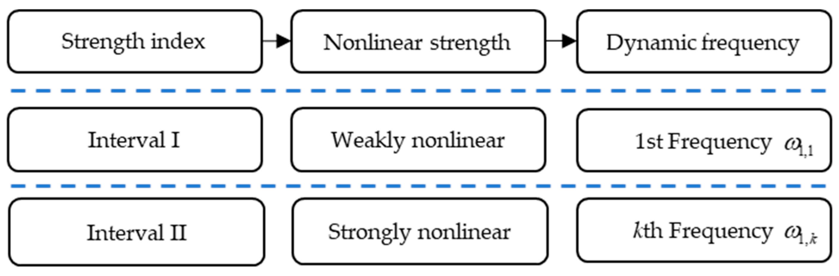
4.2. The Nonlinear Strength Index

In Table 3, a slight difference in the parameter choice will lead to a dramatic change in the nonlinear behavior. Such a change is obviously due to the relationship between the linear and nonlinear parts, which in turn decide the strategies of further computation. Accordingly, one needs an index to classify the strength of nonlinearity so that we can decide to choose the suitable algorithms of computation.

From Equations (43) and (44), the collocation points for the linear and nonlinear Hamilton equations are ${\theta }_0$ and ${\theta }_1$. Suppose ${\theta }_1=\pi /\lambda$, the absolute value $\left|\lambda -4\right|$ accordingly represents the effect of nonlinearity, for ${\theta }_0=\pi /4$. In

Table 4. Nonlinear strength indexes and nonlinear interval.

Groups	G1	G2	G3	G4
Index δ	0.22	0.28	0.43	0.62
Interval	weakly nonlinear		strongly nonlinear

, we outline a new nonlinear strength index $\delta =\left|\lambda -4\right|$ according to different parameter groups. From G₁ to G₄, the enlargement of $\delta$ synchronizes the intensification of the nonlinearity, as well as the loosing accuracy of the first order analytical approximate solutions. Then, two major nonlinear intervals are logically classified, where the boundary values $\delta =0.3$ are a coarse estimate, only for the choice of the following analytical strategies. The nonlinear strength indexes and belonging intervals from G₁ to G₄ are presented in Table 4.

$$\{\begin{array}{ll}\mathrm{I}:0<\delta <0.3& weaklynonlinearinterval,\\ \mathrm{II}:\delta >0.3& stronglynonlinearinterval,\end{array}$$

(46)

In Figure 5, we present the flow chart of approximation computation regarding δ. For example, in interval I, it just requires the first order dynamic frequency for the weakly nonlinear feature; in interval II, it demands the second order or other possible kth order dynamic frequency, $k\ge 2$, and the modified EBM results improve the accuracy of computation, for its strongly nonlinear character.

5. Conclusions

In this paper, we present a new dynamic frequency method to solve the periodic solutions for strongly nonlinear oscillators. Based on the analysis of the energy equation, the analytical approximate solutions with high accuracy are obtained through a limited trigonometric balancing progress. Moreover, we set up the strategies to find the higher-order dynamic frequency approximation as well as the modified EBM. Two examples have been solved and the analytical approximate solutions are presented to illustrate the effectiveness and applicability of the present method.

The principal merits of our approach can be summarized as follows: 1. Unlike the harmonic balance method, the influence of the higher harmonic terms is directly embodied in the expression of dynamic frequency which reduces the cumbersome steps of multiple balancing in HB; 2. the new approach is not only valid for strongly nonlinear conservative oscillators but also for non-conservative systems with limit cycles; 3. the lowest order approximations obtained by the present method are actually of high accuracy; 4. the modified energy balance method is introduced to simplify the procredure of high-order analytical computation; and 5. the nonlinear strength index provides possible choices of the avaliable analytical strategies to the general nonlinear systems.

The entire procedure can be regarded as a foundation for further nonlinear analysis, such as for fractional-order nonlinear systems or fluid-structure interaction [46,47]. These will be the topics for further research.

References

1. Rontó, A.; Rontó, M. Periodic successive approximations and interval halving. Miskolc Math. Notes 2012, 13, 459–482. [Google Scholar] [CrossRef]
2. Rontó, A.; Rontó, M.; Jana, V. A new approach to non-local boundary value problems for ordinary differential systems. Appl. Math. Comput. 2015, 250, 689–700. [Google Scholar] [CrossRef]
3. Rontó, M. Numerical-analytic successive approximation method for nonlinear boundary value problems. Nonlinear Anal. Theor. 1997, 30, 3179–3188. [Google Scholar] [CrossRef]
4. Rontó, M. On two numerical-analytic methods for the investigation of periodic solutions. Period. Math. Hung. 2008, 56, 121–135. [Google Scholar] [CrossRef]
5. Mitropolskii, Y.A.; Moseekov, B.I. Asymptotic Solutions of Partial Differential Equations; Vyshcha Shkola: Kiev, Ukraine, 1976. [Google Scholar]
6. Mickens, R.E. Oscillations in Planar Dynamic Systems; World Scientific: Singapore, 1996. [Google Scholar]
7. Bogolubov, N.N.; Mitropolski, Y.A. Asymptotic Methods in the Theory of Nonlinear Oscillations; CRC Press: New York, NY, USA, 1961. [Google Scholar]
8. Krylov, N.M.; Bogoliubov, N.N. Introduction to Nonlinear Mechanics; Princeton University Press: Princeton, NJ, USA, 1947. [Google Scholar]
9. Mahmoud, G.M. Approximate solutions of a class of complex nonlinear dynamical systems. Phys. A 1998, 253, 211–222. [Google Scholar] [CrossRef]
10. Sandri, G. A new method of expansion in mathematical physics. Il Nuovo Cimento 1965, 36, 67–93. [Google Scholar] [CrossRef]
11. Lindstedt, A. Ueder die integration einer fur die storungstheorie wichtigen differential gleichung. Astron. Nach. 1882, 103, 211–222. [Google Scholar] [CrossRef]
12. Nayfeh, A.H.; Mook, D.T. Nonlinear Oscillations; John Wiley & Sons: New York, NY, USA, 1995. [Google Scholar]
13. Belendez, A.; Pascual, C.; Mendez, D.I.; Neipp, C. Solution of the relativistic (an) harmonic oscillator using the harmonic balance method. J. Sound Vib. 2007, 311, 1447–1456. [Google Scholar] [CrossRef]
14. Garcia-Margallo, J.; Bejarano, J.D. A generalization of the method of harmonic balance. J. Sound Vib. 1987, 116, 591–595. [Google Scholar] [CrossRef]
15. Stokes, A. On the approximation of nonlinear oscillations. J. Differ. Equ. 1972, 12, 535–538. [Google Scholar] [CrossRef]
16. Garcia-Saldana, J.D.; Gasull, A. A theoretical basis for the harmonic balance method. J. Differ. Equ. 2013, 254, 67–80. [Google Scholar] [CrossRef]
17. Alam, M.S. A modified and compact form of Krylov-Bogoliubov-Mitropolskii unified method for solving an nth order nonlinear differential equation. Int. J. Nonlinear Mech. 2004, 39, 1343–1357. [Google Scholar] [CrossRef]
18. Sun, W.P.; Wu, B.S.; Lim, C.W. A modified lindstedt-poincare method for strongly mixed-parity nonlinear oscillators. Trans. ASME. J. Comput. Nonlinear Dyn. 2007, 2, 141–145. [Google Scholar] [CrossRef]
19. Chung, K.W.; Chan, C.L.; Xu, Z.; Mahmoud, G.M. A perturbation-incremental method for strongly nonlinear autonomous oscillators with many degrees of freedom. Nonlinear Dyn. 2002, 28, 243–259. [Google Scholar] [CrossRef]
20. Li, S.; Liao, S.J. An analytic approach to solve multiple solutions of a strongly nonlinear problem. Appl. Math. Comput. 2005, 169, 854–865. [Google Scholar] [CrossRef]
21. Chen, S.H.; Cheung, Y.K. A modified Lindstedt-Poincare method for a strongly non-linear two degree-of-freedom system. J. Sound Vib. 1996, 193, 751–762. [Google Scholar] [CrossRef]
22. Senator, M.; Bapat, C.N. A perturbation technique that works even when the nonlinearity is not small. J. Sound Vib. 1993, 164, 1–27. [Google Scholar] [CrossRef]
23. Amore, P.; Aranda, A. Improved Lindstedt-Poincare method for the solution of the nonlinear problems. J. Sound Vib. 2005, 283, 1115–1136. [Google Scholar] [CrossRef]
24. Belhaq, M.; Lakrad, F. Prediction of homoclinic bifurcation: The elliptic averaging method. Chaos Solitons Fractals. 2000, 11, 2251–2258. [Google Scholar] [CrossRef]
25. Wang, W.; Zhang, Q.C.; Tian, R.L. Asymptotic solutions and bifurcation analysis of the strongly nonlinear oscillation system with two degrees of freedom. J. Vib. Shock 2008, 27, 130–133. [Google Scholar]
26. He, J.H. Preliminary report on the energy balance for nonlinear oscillations. Mech. Res. Commun. 2002, 29, 107–111. [Google Scholar] [CrossRef]
27. Davod, A.G.; Ganji, D.D.; Azami, R.; Babazadeh, H. Application of improved amplitude frequency formulation to nonlinear differential equation of motion equations. Mod. Phys. Lett. B 2009, 23, 3423–3436. [Google Scholar] [CrossRef]
28. Khan, Y.; Mirzabeigy, A. Improved accuracy of He’s energy balance method for analysis of conservative nonlinear oscillator. Neural Comput. Appl. 2014, 25, 889–895. [Google Scholar] [CrossRef]
29. Younesian, D.; Askari, H.; Saadatnia, Z.; Kalami, Y.M. Frequency analysis of strongly nonlinear generalized Duffing oscillators using He’s frequency-amplitude formulation and He’s energy balance method. Comput. Math. Appl. 2010, 59, 3222–3228. [Google Scholar] [CrossRef]
30. Elias-Zuniga, A.; Martinez-Romero, O. Energy method to obtain approximate solutions of strongly nonlinear oscillators. Math. Probl. Eng. 2013, 2012, 620591. [Google Scholar]
31. Chen, Y.Y.; Chen, S.H. Homoclinic and heteroclinic solutions of cubic strongly nonlinear autonomous oscillators by the hyperbolic perturbation method. Nonlinear Dyn. 2009, 58, 417–429. [Google Scholar] [CrossRef]
32. Stoker, J.J. Nonlinear Vibrations in Mechanical and Electrical Systems; Interscience Publishers: New York, NY, USA, 1950. [Google Scholar]
33. Mickens, R.E. Iteration procedure for determining approximate solutions to nonlinear oscillator equations. J. Vib. Shock 1987, 116, 185–187. [Google Scholar]
34. Li, P.S.; Wu, B.S. An iteration approach to nonlinear oscillations of conservative single-degree-of-freedom systems. Acta Mech. 2004, 170, 69–75. [Google Scholar] [CrossRef]
35. Garcia-Saldana, J.D.; Gasull, A. The period function and the harmonic balance method. Bull. Sci. Math. 2015, 139, 33–60. [Google Scholar] [CrossRef]
36. Mickens, R.E. Turly Nonlinear Oscillations; World Scientific: Singapore, 1996. [Google Scholar]
37. Lau, S.L.; Cheung, Y.K. Amplitude incremental variational principle for nonlinear vibration of elastic system. ASME J. Appl. Mech. 1981, 48, 959–964. [Google Scholar] [CrossRef]
38. Wu, B.S.; Li, P.S. A method for obtaining approximate analytic periods for a class of nonlinear oscillators. Meccanica 2001, 36, 167–176. [Google Scholar] [CrossRef]
39. Wu, B.S.; Li, P.S. A new approach to nonlinear oscillations. ASME J. Appl. Mech. 2001, 68, 951–952. [Google Scholar] [CrossRef]
40. Yamgoué, S.B. On the harmonic balance with linearization for asymmetric single degree of freedom non-linear oscillators. Nonlinear Dyn. 2012, 69, 1051–1062. [Google Scholar] [CrossRef]
41. Li, L. Energy method for computing periodic solutions of strongly nonlinear systems-autonomous systems. Nonlinear Dyn. 1996, 9, 223–247. [Google Scholar] [CrossRef]
42. Lev, B.I.; Tymchyshyn, V.B.; Zagorodny, A.G. On certain properties of nonlinear oscillator with coordinate-dependent mass. Phys. Lett. A. 2017, 381, 3417–3423. [Google Scholar] [CrossRef]
43. Wu, Y.; He, J.H. Homotopy perturbation method for nonlinear oscillators with coordinatedependent mass. Results Phys. 2018, 10, 270–271. [Google Scholar] [CrossRef]
44. Ganji, D.D.; Esmaeilpour, M.; Soleimani, S. Approximate solutions to Van der Pol damped nonlinear oscillators by means of He’s energy balance method. Int. J. Comput. Math. 2010, 9, 2014–2023. [Google Scholar] [CrossRef]
45. Ismail, G.M. An analytical technique for solving nonlinear oscillators of the motion of a rigid rod rocking bock and tapered beams. J. Appl. Comput. Mech. 2016, 2, 29–34. [Google Scholar]
46. Ding, H.; Chen, L.Q. Galerkin methods for natural frequencies of high-speed axially moving beams. J. Sound Vib. 2010, 329, 3484–3494. [Google Scholar] [CrossRef]
47. Ding, H.; Chen, L.Q.; Yang, S.P. Convergence of galerkin truncation for dynamic response of nite beams on nonlinear foundations under a moving load. J. Sound Vib. 2012, 331, 2426–2442. [Google Scholar] [CrossRef]
Figure 1. Comparison of analytical approximations and numerical solution for γ = 1 , A = 0.8 in Equation (14).
Symmetry 11 00676 g001
Figure 2. Absolute errors of analytical approximations for different orders (a) the first order approximate solution and (b) the second order approximate solution.
Symmetry 11 00676 g002
Figure 3. Comparison of approximate solutions to Equation (33) for (a) α = 0.1 ; (b) α = 0.3 ; (c) α = 0.5 and (d) α = 0.8 : Runge-Kutta method (red solid line), Homotopy Perturbation method (orange dashed line), the present method (black dotted line).
Symmetry 11 00676 g003
Figure 4. Comparison of approximate solutions of Equation (45) under different sets of parameters: (a) G1; (b) G2; (c) G3; (d) G4; Runge-Kutta method (red solid line), the first order dynamic frequency method (black dotted line), modified energy balance method with a1 (blue dashed line).
Symmetry 11 00676 g004aSymmetry 11 00676 g004b
Figure 5. The skeleton diagram of the approximation strategy.
Symmetry 11 00676 g005