Abstract
During the construction of prefabricated building, there are some problems such as a time consuming, low-level of automation when precast concrete members are assembled and positioned. This paper presents vision-based intelligent assembly alignment guiding technology for columnar precast concrete members. We study the video images of assembly alignment of the hole at the bottom of the precast concrete members and the rebar on the ground. Our goal is to predict the trajectory of the moving target in a future moment and the movement direction at each position during the alignment process by assembly image sequences. However, trajectory prediction is still subject to the following challenges: (1) the effect of external environment (illumination) on image quality; (2) small target detection in complex backgrounds; (3) low accuracy of trajectory prediction results based on the visual context model. In this paper, we use mask and adaptive histogram equalization to improve the quality of the image and improved method to detect the targets. In addition, aiming at the low position precision of trajectory prediction based on the context model, we propose the end point position-matching equation according to the principle of end point pixel matching of the moving target and fixed target, as the constraint term of the loss function to improve the prediction accuracy of the network. In order to evaluate comprehensively the performance of the proposed method on the trajectory prediction in the assembly alignment task, we construct the image dataset, use Hausdorff distance as the evaluation index, and compare with existing prediction methods. The experimental results show that, this framework is better than the existing methods in accuracy and robustness at the prediction of assembly alignment motion trajectory of columnar precast concrete members.
1. Introduction
Planning and decision-making are important abilities for an artificial intelligence system. Motion prediction and guidance based on images is the hot issue in the field of computer vision. With the development of prefabricated buildings, artificial intelligence is gradually being applied to the human-computer interaction system in the construction site of prefabricated buildings to assist in the judgment and operation of some instructions. The research background of this paper is the installation of column-prefabricated members. There is a hole at the bottom of the precast member, and our task is to align the hole to the rebar on the ground. In the process of assembly building construction, after the prefabricated component is hoisted to the designated area, the alignment of the prefabricated component connection hole and the rebar on the ground is a special peg-in-hole assembly problem, as shown in Figure 1. Therefore, it has become the most important problem that restricts the intelligent development of the assembly building construction.
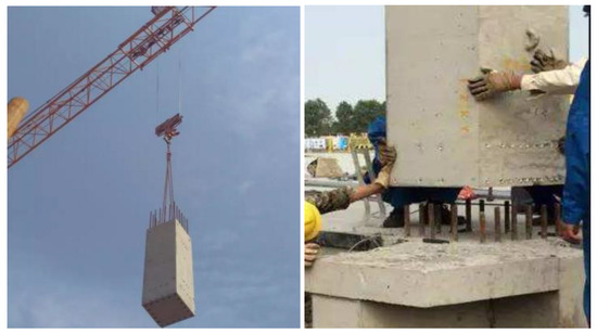
Figure 1.
Assembly of column prefabricated component.
As Figure 1 shows, the angle of the embedded hole at the bottom of the precast concrete members and the reinforcement is close to the ground, which is difficult for human eyes to observe. Therefore, the intelligent guidance technology is very necessary here. So we built a small laboratory to simulate the assembly of column prefabricated components in the laboratory to research the guiding technology. At present, the guiding technology of peg-in-hole assembly is mainly divided into two types: contact and non-contact. Contact alignment mainly relies on sensor feedback data for position adjustment and guidance, while non-contact alignment mainly uses visual data for guidance.
1.1. Assembly Technologies
Zhang [1] used a torque sensor data feedback combined with random search method to search for the hole position at the adjustment phase. This obtains a guiding direction of the next random search in iterations. The purpose of the orientation adjustment is to align the shaft with the hole to reduce torque and finally make the random search converges to a reasonable value. The search phase of this method is time-consuming and sometimes difficult to converge. Visual orientation needs to be calibrated, and there is a calibration error. Kim et al., [2] proposed that visual servo could compensate the calibration error of the camera, and the eye-in-hand positioning system was adopted in this paper. But the axis would usually block the hole when the robot approached it. A visual servo needs image acquisition, image processing, feature extraction and reconstruction of three-dimensional information from two-dimensional information. The data to be processed is huge. It relies on image consistency and is sensitive to the external environment. When the assembly environment changes, it requires three-dimensional remodeling of object position, which is complex and time-consuming. For component assembly, the change of assembly environment or assembly object is a frequent occurrence.
1.2. Computer Vision
In recent years, technologies such as deep learning and computer vision have gradually become research hotspots and have been applied to tasks such as intelligent assembly and automatic fetching. P. Ðurović [3] proposed a two-step hand-eye calibration visual servo system, and a simple grasp planning method based on vision. The method is designed for low-cost visually oriented robots, the positioning function is realized based on a visual servo, the tag tracking and depth information is provided by the rgb-d camera, and there are no encoders or other sensors. However, the rgb-d image of the object obtained by this method is greatly affected by the environment. When the image noise is large, the edge depth information of the object is easily lost. Wan [4] proposed a multi-mode visual intelligence system for mechanical assembly which consists of two stages. The key part of the system is the precision of 3d vision detection, which will be affected when gray-scale distortion occurs, matching problems of special structure covering a scene [5]. Obviously, due to the characteristics of few sensors and simple and convenient application, the intelligent system based on visual images has been applied to various fields [6,7,8]. Cireşan [9] combine various Deep Neural Networks (DNNs) trained on differently preprocessed data into a multi-column DNN, use supervised learning to identify and classify traffic signs. Deep Convolutional Neural Network (DCNN) learning needs a lot of annotated data, ND in order to solve the problem of high cost of image annotation, Wei [10] propose a simple to complex (STC) framework in which only image-level annotations are utilized to learn DCNNs for semantic segmentation. The saliency maps can be automatically obtained by existing bottom-up salient object detection techniques, where no supervision information is needed. However, whether the weak supervision method is effective or not largely depends on the compensation method of information loss in the training process [11]. Wong [12] proposed a colour image enhancement technique introduced in their work aims at maximizing the information content within an image, whilst minimizing the presence of viewing artefacts and loss of detail. Singh [13] presents two novel contrast enhancement approaches using texture regions-based histogram equalization. These methods improve the visual appearance of the image for better visual interpretation to assist in subsequent image-processing tasks (analysis, detection, recognition and prediction).
1.3. Modeling and Prediction Based on Deep Learning
An intelligent vision system should not only have simple image modeling and understanding ability, but also have the ability to perceive and predict based on the existing image information. Jazayeri [14] describes a comprehensive approach to localize target vehicles in a video under various environmental conditions. Subsequently, based on the convolutional neural network, researchers proposed the target detection algorithms such as SSD (Single Shot MultiBox Detector) [15,16] and You Only Look Once(YOLO) [17]. Leng [18] aiming at the problem that a small target is difficult to detect, and the SSD algorithm is improved, used two-way transfer of feature information and feature fusion to enhance the network. Fu [19] combine a state-of-the-art classifier with a fast detection framework. Dominguez [20] uses a convolutional neural network (CNN) to realize the reliable detection of pedestrians in a specific direction. They proposed a cnn-based technology that uses existing pedestrian detection technology to generate a sum difference framework, which is used as the input of CNN networks (such as AlexNet, GoogleNet and ResNet). In recent years, people have done a lot of research on data processing and prediction based on deep learning [15,21,22]. In order to gain the ability to make inferences from complex scenarios, as humans, Walker [23] proposed a simple visual prediction method, which combines intermediate visual elements with the validity of time modeling. It can not only predict possible motion in the scene, but also predict the change of object appearance over time. The CNNs have given the state-of-the-art performance on various two-dimensional image processing and prediction tasks [24,25,26,27,28]. At present, a deep learning framework for motion direction and trajectory prediction is mainly applied in panoramic video head motion prediction [7], and the prediction and planning of the motion path of moving objects [8]. Xu [7] found that deep reinforcement learning (DRL) can be applied to predict head movement (HM) positions, via maximizing the reward of imitating human HM scanpaths through the agent’s actions. Yoo [8] considered moving dynamics of co-occurring objects for path prediction in a scene that includes crowded moving objects. He presented an algorithm to find the future location of any target object by utilizing the unsupervised learning results from the model.
In this paper, we use image processing combined with deep learning technology to predict the motion trajectory and direction of moving targets according to the assembly image sequences, and proposes a visual intelligent guiding technology for peg-in-hole alignment of columnar precast concrete members. As Figure 2, the methods for trajectory prediction contain three components: (1) Image preprocessing, (2) understanding the scene and object detection, (3) and inferring the motion orientation of moving targets based on the information obtained from an image. In this paper, a recognition and prediction framework based on a convolution network is established to solve the prediction problem of assembly trajectory and direction. In this work, we need to capture image sequences in the assembly video operated by experts, automatically learn these prior knowledge, and further plan the motion trajectory. Prior knowledge includes the detection of a target area of interest and the prediction of a moving target’s trajectory and direction.
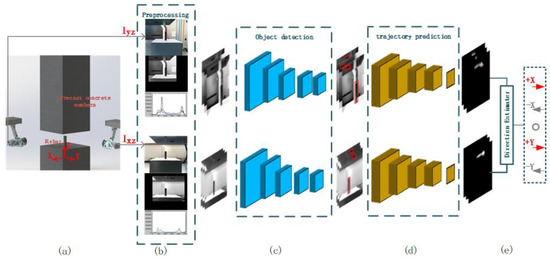
Figure 2.
Total process of our approach: (a) Get the coordinate image Iyz of X direction and Ixz of Y direction. (b) Preprocessing: mask processing and histogram equalization. (c) Object detection framework. (d) Trajectory prediction framework. (e) Direction estimator. The assembly coordinate system X-Y-Z established with the steel bar as the dot.
2. Our Approach
Our goal is to establish a framework to solve the prediction problem of motion trajectory and direction of a moving target. Firstly, we use mask technology and histogram equalization to preprocess the image. Secondly, the target position is detected through the target detection model. The position matching model is used to predict the position and direction of the moving target. As shown in Figure 3, we get the assembly images I = {Iyz, Ixz} in X and Y directions in the assembly coordinate system, define the embedded hole at the bottom of the precast concrete members as moving target C, and define the reinforcement as fixed target B. After the object detection model, we obtain bounding boxes of fixed target B = (xb, yb, wb, hb) and moving target C = (xc, yc, wc, hc). xb, yb, wb, hb are respectively the center point coordinate, the width, and the height of bounding box of fixed target B. xc, yc, wc, hc are respectively the center point coordinate, the width, and the height of the bounding box of moving target C.
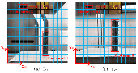
Figure 3.
Coordinate image Iyz of X direction and Ixz of Y direction. The embedded hole at the bottom of the precast member is defined as moving target C, and reinforcement is defined as fixed target B.
The image coordinate systems y-z and x-z are established along the X and Y directions in the assembly coordinate system, respectively, and the images Iyz and Ixz are obtained. We formalize the original scene into a grid diagram, as shown in Figure 3. Ds is composed of a series of adjacent position block diagrams, so that each block corresponds to a specific position Si of the scene. We call Ds the decision area, so as to represent the future appearance position of the moving target. The higher excitation value is, the higher matching probability between the moving target and the position will be. According to Figure 3 (a), the movement direction of the moving target in the X direction in the future can be obtained. Similarly, according to Figure 3 (b), the movement direction of the moving target in the Y direction in the future can be obtained. The end point of the moving target trajectory is matched with the fixed target. Trajectory prediction terminates when the center abscissa of moving target bounding box is equal to the center abscissa of a fixed target bounding box.
Therefore, the trajectory prediction problem of assembly alignment is transformed into position matching and direction judging. Establish the loss function:
R is the cost equation, Si represents the specific position of the block in the image corresponding to the scene.
2.1. Object Detection Network
First, we establish an object detection model. Due to the particularity of the objects tested in this paper, the existing detection algorithms should be improved and optimized to make them adapt to our target detection. The main process of current mainstream detection algorithms [29,30,31] can be divided into the following parts: (1) the depth feature of the whole input image is extracted by the depth neural network; (2) feature capture boxes of different sizes were designed for depth feature maps of different scales. These boxes were matched with the real target frame for training; (3) predicting the target category and the real target frame by extracting the features of depth feature graph corresponding to these feature capture boxes; (4) filtering and outputting the best prediction results.
The object detection model in this paper is improved on the basis of SSD [16], and its detection and recognition process can be solved by the same network. SSD (Single Shot MultiBox Detector) is a method for detecting objects in images using a single deep neural network. It discretizes the output space of bounding boxes into a set of default boxes over different aspect ratios and scales per feature map location. At prediction time, the network generates scores for the presence of each object category in each default box and produces adjustments to the box to better match the object shape.
It can be seen that the input of the target detection model in this paper is the image sequence of the video. Use a basic deep learning model network to extract features from the whole image, and the deconvolution layer is added to the end of the feature layer, which improved detection accuracy of large scale background, especially for small targets. As shown in Figure 4, the object detection network includes conv1, pool1, conv2_2, conv3_2, conv4_2, conv5_2, and DSSD layers. There is a pooling layer behind conv1. The conv2_2 layer was disposed of with 3 × 3 × 256 s2 convolution kernel, where s2 means that convolution step length is 2. The convolution process here uses the atrous algorithm, and then take the convolution operation again with the convolution kernel of 1 × 1 × 128 to get the feature graph for detection and recognition. The next step is to extract the local features from the multi-scale feature graph and use the obtained features to predict the results. All potential targets were detected by feature fusion using the improved SSD, and then the improved SSD detection results were re-evaluated using the improved visual reasoning method. The proposed end-to-end connection allows feature maps of each output layer to contain rich features, details and semantic information [19].
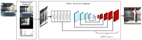
Figure 4.
Object detection network includes conv1, pool1, conv2_2, conv3_2, conv4_2, conv5_2, and DSSD layers. There is a pooling layer behind conv1. The conv2_2 layer was disposed with 3 × 3 × 256-s2 convolution kernel, where s2 means that convolution step length is 2. The convolution process here uses the atrous algorithm.
The SSD training objective is derived from the MultiBox objective but is extended to handle multiple object categories. The overall objective loss function is a weighted sum of the localization loss (loc) and the confidence loss:
where N is the number of matched default boxes. If N = 0, wet set the loss to 0. The localization loss is a Smooth L1 loss between the predicted box (l) and the ground truth box (g) parameters. The weight term α is set to 1 by cross validation.
is used to measure the predictive performance of bounding boxes. represents the deviation between the real target frame of the j-th target and the frame of the feature capture box, , represents the coordinate of the center point of the frame, indicates the width and height of the frame.
is used to measure the recognition performance, indicates whether the i-th box matches the boundary box of the j-th target of the object p.
Due to the particularity of the object extracted in this paper, we reset the proportion of feature capture boxes. Assuming that there are n characteristic graphs, the scale parameters can be expressed as follows:
smin is minimum scale parameter, smax is maximum scale parameter. Since the detection targets in this paper are circular holes and rebar, the length-width ratio parameter of bounding boxes is set to .The bounding boxes include the information of center point coordinates (x,y), width and height (w,h) and confidence.
2.2. Trajectory Prediction Network
We built a reward network to model the interaction among moving targets (holes), fixed targets (rebar), and moving regions in the scene. Intuitively, when the fixed target is on the left side of the moving target, the moving target should be moved to the left. When the fixed target is on the right side of the moving target, the moving target should be moved to the right. In the training phase, we develop a depth context model called the trajectory prediction framework to learn object context information from the sequence of images. As shown in Figure 4, after extracting features from the target position image through the convolutional layer, the two-dimensional array was transformed into a one-dimensional array through the flatten layer. This is because the processing of two-dimensional array by Long Short-Term Memory (LSTM is not only time-consuming, but also requires a large amount of computation. LSTM processes one-dimensional data which have sequence characteristics. After processing is complete, the data are transformed into a two-dimensional array by reshape function and output them as a costmap.
We use multi-layer convolutional neural network to extract the mapping relationship between assembly image sequence features and the trajectory of moving target. In the testing phase, we can get the matching likelihood r of the prediction area and actual area of the moving target:
Image sequence number m ranging from 1 to M. D defines the patch difference, is the central coordinate of the prediction patch, is the center coordinate of the actual patch, and ρ is the standard deviations of Gaussian distributions, as the hyper-parameters.
In our approach, global-shared parameters are updated via an accumulating gradient [30]. we can optimize reward r as follows:
In this paper, global-shared parameters are the weight coefficients of the neural network. represents the gradient. The convolution operation ensures that each pixel has a weight coefficient, which is shared by the whole convolution layer. In the process of training neural networks, they are constantly updated to make the predicted output close to the actual output.
Finally, based on the above equations, RMSProp [7] is applied to optimize rewards in the training data. RMSProp is an adaptative learning rate method that has found much success in practice which proposes to normalize the gradients by an exponential moving average of the magnitude of the gradient for each parameter:
where 0 < α < 1 denotes the decay rate. v is the state variable. The update step is given by
where is the learning rate and is a damping factor.
For the image sequence t = m, we can generate reward equation for Ic by inputting the sliding window into the network:
Rreward(Si) is the reward for each position Si. represents a sliding window. The larger value means the higher reward for that position, namely the higher probability the object will reach that position in the future. represents the forward propagation function, and is learning rate.
Different objects may have same relationships with the different region of the scene. Rreward(Si) is used to establish the cost equation:
α is the excitation attenuation coefficient. η is the equilibrium coefficient. Set it to 5, as the scale of reward r is [0:1].
End point position matching. Firstly, we know the end point of the movement is above the reinforcement instead of touching it. According to the above, as Figure 5, we have formalized the semantic understanding of images into object detection and position matching. By contrast with those mentioned in papers [7,8] earlier, the image reward modeling in our paper is not only related to the moving target, but also with the fixed target. In this paper, aiming at the uncertainty of the visual context model in the prediction of the path ending point, the end point position matching equation is established as the constraint term of the loss function according to the principle of pixel matching of the moving target and fixed target. When the abscissa of moving target Ic in the image is equal to the abscissa of fixed target Ib, we consider that this point is the optimal endpoint position in the decision region DS. Set the end point position matching equation as follows:
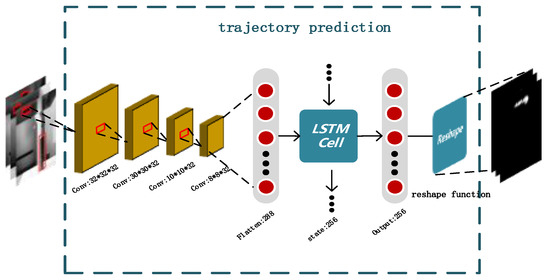
Figure 5.
Prediction network: after extracting features from the target position image through the convolutional layer, the two-dimensional array was transformed into a one-dimensional array through the flatten layer. Long Short-Term Memory (LSTM) processes one-dimensional data which have sequence characteristics. After processing is complete, the data are transformed into a two dimensional array by reshape function and output them as costmap.
When t = M, the end point position of the trajectory . This equation indicates that the moving target point whose abscissa is closest to the abscissa of the fixed target in the trajectory is the optimal endpoint, and the predict trajectory is closest to the real trajectory.
According to the above mentioned formulas (6) and (7), we describe the loss function of the trajectory as the following equation:
is cost equation, is Constraint term, we call this the endpoint position matching equation. According to experience, is set to 0.2.
Direction estimator. Determine the motion direction of each predicted position, and establish the direction discriminant equation as follows:
is the abscissa of the moving target at time t, is the abscissa of the fixed target. is the motion direction of the moving target in the assembly coordinate system. We give the trajectory prediction algorithm as Table 1.

Table 1.
Trajectory prediction algorithm.
3. Experiments
3.1. Dataset
We build CNNs based on the TensorFlow. In this section, we set up the experimental platform as shown in Figure 6, and establish the image data set of the hole and reinforcement.
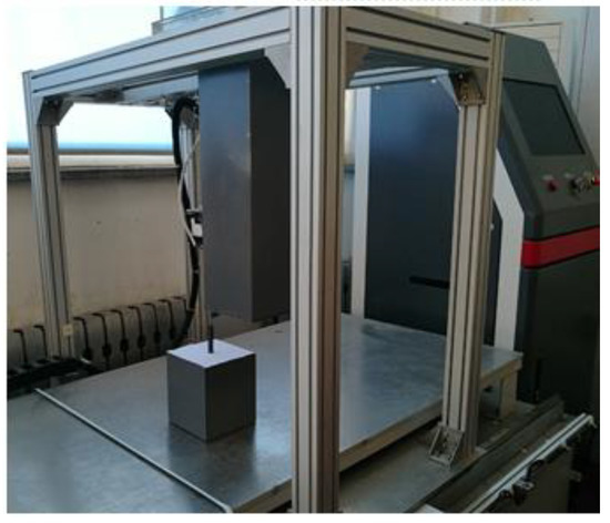
Figure 6.
Laboratory furniture.
We divide peg-in-hole alignment motions into 9 types according to their relative positions, as shown in Figure 6. The database contains 120 video sequences. We intercept 7500 associated images from video sequences and conduct clipping processing to adapt to our network and mark the targets in images manually. We store tag files in annotations files, which contain information about the location of the target. We store the training and test images in the Images file. The training and validation data sets accounted for 60% and the test data set accounted for 40%.
As in Figure 7, we placed two cameras aligned with the axis of the reinforcement. However, the camera placement process needs some positioning equipment to assist it, which can not only ensure the accuracy of data acquisition but also increase the flexibility of placement. In this paper, we use the electronic level ruler for construction to assist the camera placement. The electronic level ruler for construction is an intelligent inclination measuring instrument developed by using digital angle sensor and many modern technologies. It has the function of measuring absolute angle, relative angle, slope and level. The electronic level ruler for construction is placed on the platform to make it vertical to the reinforcement, and draw the vertical line, place the camera on the vertical line and the distance and height are determined according to the image.
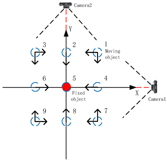
Figure 7.
Location of reinforcement and hole. The blue dotted line in the figure represents the location of the moving target (hole), red dot represent fixed targets (rebar). Camera1 and Camera2 are placed respectively in the X and Y directions of the assembly coordinate system.
3.2. Preprocessing
Because the contrast and brightness of the training samples are not consistent, the image often appears bright or dark (as shown in Figure 8), which will have a great impact on the recognition effect of the network. Histogram equalization is used for some images to enhance the training effect. Histogram equalization is to transform the gray histogram of the original image from a relatively concentrated gray range into a uniform distribution within a gray range. Histogram equalization is to stretch the image non-linearly and reassign the pixel value of the image, so that the number of pixels in a certain gray scale is approximately the same.
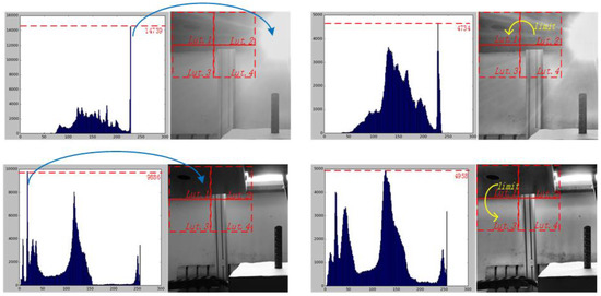
Figure 8.
The left side of the graph is the image and histogram before processing, and the right side is the image and histogram after processing. In the first line, the maximum number of pixels before processing is 14,739, and the maximum number of pixels after processing is 4734. In the second line, the maximum number of pixels before processing is 14,739, and the maximum number of pixels after processing is 4734. As can be seen from the figure, the processed image has a more balanced distribution of pixels. The yellow arrow indicates that an image block whose average pixel value exceeds the intensity limit allocates redundant pixels to its adjacent image blocks.
We use r and s to denote the gray level of the original image and the gray level of the histogram after equalization. For images, the normalized gray level was distributed in the range of . In the [0,1] interval, r is transformed as follows:
The inverse transformation from s to r is expressed in the following form:
The probability density of r is , and the probability density of s can be calculated from :
The transformation function is expressed as:
ω is integral variable and is the cumulative distribution function of r.
Calculate the derivative of r in the formula:
Take the result into (12), we can get:
It can be seen that the probability density of the variable s in its definition domain is evenly distributed after transformation. Therefore, using the cumulative distribution function of r as the transformation function, we can produce a gray level image with uniform probability density.
Processing flow: Step 1. The image boundary is extended so that it can be exactly segmented into subblocks. Assume that the area of each sub-block is tileSizeTotal, The subblock coefficient is . Handle the default limit limit = MAX (1, limit × tileSizeTotal/256);
Step 2. For each subblock, calculate the histogram;
Step 3. Use the preset limit value to limit the gray level of each subblock histogram, and count the number of pixels in the histogram that exceeds limit value;
Step 4. Calculate the cumulative histogram tileLut for each subblock, tileLut[i] = sum[i] × LutScale; sum[i] represents the number of pixels in the cumulative histogram; LutScale ensures that tileLut has a value of (0, 255).
Step 5. Traversing each point of the original image, consider the tileLut of subblock of this point and the right, lower and lower right subblocks, take the original gray value as the index to get 4 values, and then do the bilinear interpolation to get the gray value after the transformation of the point.
3.3. Training
We input the sorted image sequence into the target detection network in groups, obtain the significant target position, and then input it into the direction matching network. The cost map of the trajectory of a moving target is generated as the output of the trajectory prediction network. Finally, the results of motion direction were output after direction estimator.
- (1)
- Input the image sequence with target annotation into the object detection network, and supervised learning is used to train and output images with significant target frames.
- (2)
- After grouping and sorting the significant target image sequences, they are input into the trajectory prediction network for training and feature extraction. Calculate reward from the reward estimator with (3), which measures how close the prediction region to the ground-truth region. Generate cost map.
- (3)
- Obtain the motion directions through the direction estimator.
3.4. Results
Trajectory prediction. Figure 9 shows some qualitative results generated by our method on different positions of the evaluation set. The cost map indicates the higher probability of moving target appearing in some places, and the trajectory of moving target in the future is formed by connecting the higher probability regions. It can be seen from the cost map that the predicted motion trajectory not only changes in the abscissa of the image, but also changes in the ordinate, and breakpoints will occur when the ordinate of the trajectory changes. This is because during the alignment of the moving target (hole) and fixed target (reinforcement), the movement of the moving target in the perpendicular direction to the camera will change its y-coordinate projection in the image coordinate system, but the change ratio of the y-coordinate projection in the image is significantly smaller than that of the x-coordinate projection. Visually, the predicted paths are close to our human’s inference. In general, our framework is able to predict the trajectory and direction of motion correctly.
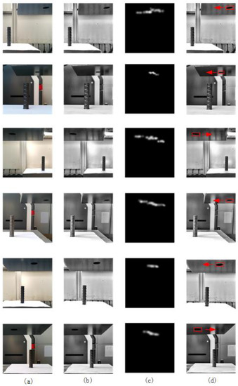
Figure 9.
(a) Represents the original image processed by mask. (b) Represents the gray image after histogram equalization processing. (c) Represents costmap of motion trajectory. (d) Represents the result of direction estimator.
Confusion matrix. In order to show the prediction performance of the network, we use a confusion matrix to record data. The confusion matrix is a situation analysis table which summarizes the prediction results of the model in machine learning. The records in the data set are aggregated in the form of a matrix according to the two criteria of real classification and predicted classification. We represent the prediction results of the network model for each trajectory point in the form of binary classification, as shown in Figure 10.
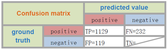
Figure 10.
The rows of the matrix represent the ground truth, and the columns of the matrices represent the predicted values. TP = number of true positives, TN = number of true negatives, FN = number of false negatives, and FP = number of false positives.
From Figure 10, we can see that the number of true positives is highest, and the number of false negatives is more than number of false positives, which shows the missed detections are more than the false detections. Due to the large number of true negatives, we do not give the statistics of TN.
Closed loop trajectory. Although previous experiments have described the predicted trajectory at different positions, the analysis of the closed-loop trajectory of the moving target in the assembly alignment task is also of great significance. In this set of experiments, we performed this evaluation by depicting two sets of three-dimensional trajectories based on the predicted trajectories.
The results that have been obtained are represented in Figure 11. The green trajectory in the figure is the line from the moving target point to the fixed target point, which is also the ground truth trajectory. The red curve represents the trajectory we predicted. It can be seen from the results that the trajectory we predicted can connect the moving target point with the fixed target point, which indicates that the assembly work can be successfully completed according to the trajectory we predicted. In addition, it can be seen that the predicted trajectory curve is not very different from the ground truth trajectory, which indicates that our prediction method can adapt to different assembly conditions and can complete assembly operations efficiently.
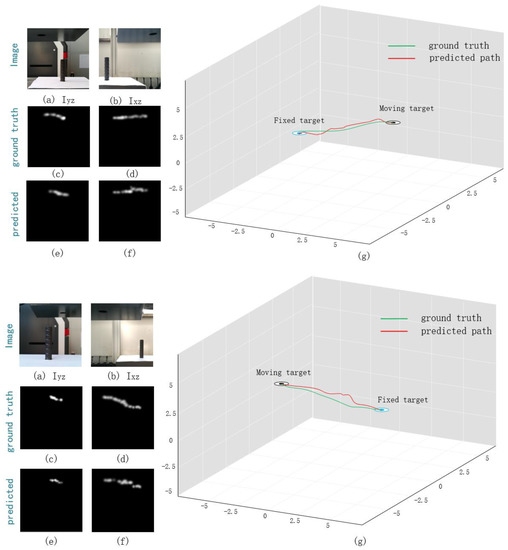
Figure 11.
Closed loop trajectories of two groups of assembly motions: (a) image of Iyz; (b) image of Ixz; (c) ground truth trajectory of Iyz; (d) ground truth trajectory of Ixz; (e) predicted trajectory of Iyz; (f) predicted trajectory of Ixz; (g) closed loop trajectory.
Contrast Experiment: Since there are no works on the motion trajectory prediction and modeling of peg-in-hole alignment of precast concrete members, we can only compare the method in this paper with the two existing prediction methods [7,8] in our data set. Since the existing prediction methods are different from the prediction tasks in this paper, the methods and parameters provided by them are used for experiments. The results are shown in Figure 12. The first row are images after mask processing, and it can be seen that the images processed by the mask remove the most useless background.
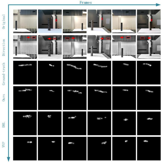
Figure 12.
Some qualitative comparison results. Each column represents a sample. First row represents the image after the mask processing. Second row represents the direction discrimination result. The third row represents ground-truth trajectory. The other rows respectively show the predicted trajectories generated by different approaches: ours, deep reinforcement learning (DRL) and Visual Value Prediction (VVP).
As Figure 12 is shown, the second row are the grayscale images processed by histogram equalization, which contain the result of direction discrimination. The third row shows the actual trajectory images manually annotated. We mark the trajectory points from different expert videos and that is why the points of ground truth row have different intensities. Brighter points indicate that these points appear more frequently in all expert videos, while darker points indicate that these points appear less frequently all expert videos. The fourth row shows the cost maps generated by our method, in this paper, the excitation value r of each position in the image is extracted by using the sliding window, and then the corresponding cost value of each position is calculated by using the cost equation (16). When the predicted position of the moving target is close to the actual position, the cost value of this position is relatively low. Therefore, the location with a high pixel value in the cost map indicates that the moving target (hole) will have a high probability to appear at this location in the future. It can be seen from Figure 12 that the predicted trajectory is roughly the same as the actual trajectory, and the end position of the predicted trajectory is more accurate compared with the other two methods, which also indicates the correctness of the end point pixel matching method used in this paper. But there are some breakpoints in the middle part of the trajectory, and the breakpoint part usually occurs where the ordinate of the trajectory changes. This indicates that the movement of the moving target (hole) in the perpendicular direction to the camera reduces the prediction accuracy of the network, while the movement of the moving target (hole) in the parallel direction to the camera has no influence on the prediction accuracy.
The fifth row shows the trajectory prediction images generated by the [7] method. The breakpoint condition of this trajectory is serious, and the predicted trajectory has a low matching degree with the actual trajectory. The sixth row are the trajectory prediction images generated by the [8] method. It can be seen that this method is not suitable for the trajectory prediction of peg-in-hole alignment. It can be seen from the comparison images that the predicted trajectory generated by the method in this paper has the highest matching degree with the actual trajectory, and it is obviously better than the other two methods on the trajectory prediction of peg-in-hole alignment.
Hausdorff distance. In order to make an explicit quantitative comparison between our method and the existing methods, in this paper, Hausdorff distance [32] is used as the evaluation metric to measure the matching degree between the predicted trajectory and the actual trajectory. Hausdorff distance is a measure to describe the similarity between two sets of points. It is a definition form of the distance between two sets of points: Suppose there are two sets A = {a1, …, ap} and B = {b1, …, bq}, the Hausdorff distance between the two sets of points is defined as
‖·‖ is the normal form of distance between point set A and point set B.
The quantitative comparison results are shown in Table 2. It can be seen from the table that the Hausdorff distance between the predicted trajectories proposed in this paper and the actual trajectories is the smallest, which indicates that their matching degree is the highest. In order to further verify the validity of the end point position matching equation, an experimental result which removes the end point position matching equation is shown as Ours(w/o). It can be seen from the results that after removing this equation, the Hausdorff distance of Ours(w/o) increases and the matching degree decreases, which is close to the result of DRL. This indicates that the end point position matching equation will significantly enhance the prediction performance of our network.
Table 2.
Quantitative comparison results.
Success rate is the fraction or percentage of success among a number of tests. Some assembly operations need to be completed outdoors. The effect of wind load on assembly operations is considered here. When the wind speed reaches a certain level, it will cause the members to sway, which will affect the success rate of the assembly. We test it under different wind speeds, and count the results of the experiments, and compar the success rate of several methods, to give a much better indication of the usability, as in Table 3.
Table 3.
Success rate under different wind speed.
Visual servo as a traditional method of visual guidance is added for comparison. It can be seen from the table that our method has the highest success rate, but with the increase of wind speed, the success rate gradually decreases, but is still higher than the other methods. This shows that the wind speed has a great influence on the method. In this paper, a neural network is developed to imitate the assembly process of human beings. This emphasizes the interaction between the vision system and its environment. It does not use other sensors for closed-loop control. We hope to improve its assembly success rate through continuous training, and ultimately make it have the assembly ability close to human beings.
4. Conclusions
In this paper, a deep learning framework is proposed to solve the trajectory prediction problem of the moving target (hole at the bottom of precast concrete members). We build an object detection model, trajectory prediction model and specific inference algorithms to predict the trajectory and motion direction of the moving target. In addition, the proposed object detection was combined with the LSTM network to model the moving target image sequence, and at the same time to carry out the deep feature learning of visual representation, which greatly improved the ability to understand the assembly scene.
(1) Aiming at the problem of complex backgrounds, difficult to detect small targets, and influence of the sunlight in assembly images, we use mask and adaptive histogram equalization to preprocess images. Additionally, we analyze the influence of different wind speeds on the success rate of assembly testing. Based on the image sequence, a unified image coordinate system is established and the image quality is greatly improved.
(2) Aiming at the low position precision of trajectory prediction based on the context model, we propose the end point position matching equation according to the principle of end point pixel matching of the moving target and fixed target, as the constraint term of the loss function to improve the prediction accuracy of the network.
(3) Hausdorff distance is introduced as an indicator in the comparative experiment to evaluate the performance of the model in the task of predicting the assembly alignment motion trajectory, and analyze the characteristics and the causes of breakpoints in the trajectory. The results show that the method proposed in this paper has higher prediction accuracy and robustness in the aspect of motion prediction of precast concrete members compared with the existing methods.
Author Contributions
Authors K.Z. and S.T. conceived and designed the model for research and pre-processed and analyzed the data and the obtained inferences. Authors H.S. processed the data collected and wrote the paper. Author S.T. checked and edited the manuscript. The final manuscript has been read and approved by all authors.
Funding
This research was funded by The National Key R & D Program of China, grant number 2017YFC0703903, 2017YFC0704003 and the National Natural Science Foundation of China, grant number 51705341, 51675353.
Acknowledgments
The authors are grateful to the editors and the anonymous reviewers for providing us with insightful comments and suggestions throughout the revision process.
Conflicts of Interest
The authors declare no conflict of interest.
References
- Zhang, X.; Zheng, Y.; Ota, J.; Huang, Y. Peg-in-Hole Assembly Based on Two-phase Scheme and F/T Sensor for Dual-arm Robot. Sensors 2017, 17, 2004. [Google Scholar] [CrossRef] [PubMed]
- Kim, Y.L.; Song, H.C.; Song, J.B. Hole detection algorithm for chamferless square peg-in-hole based on shape recognition using F/T sensor. Int. J. Precis. Eng. Manuf. 2014, 15, 425–432. [Google Scholar] [CrossRef]
- Ðurović, P.; Grbić, R.; Cupec, R. Visual servoing for low-cost SCARA robots using an RGB-D camera as the only sensor. Automatika: Časopis za Automatiku, Mjerenje, Elektroniku, Računarstvo i Komunikacije 2018, 58, 495–505. [Google Scholar] [CrossRef]
- Wan, W.; Lu, F.; Wu, Z.; Harada, K. Teaching Robots to Do Object Assembly using Multi-modal 3D Vision. Neurocomputing 2017, 259, 85–93. [Google Scholar] [CrossRef]
- Teng, Z.; Xiao, J. Surface-Based Detection and 6-DoF Pose Estimation of 3-D Objects in Cluttered Scenes. IEEE Trans. Robot. 2016, 32, 1347–1361. [Google Scholar] [CrossRef]
- Kitani, K.; Ziebart, B.; Bagnell, J.; Hebert, M. Activity forecasting. In Proceedings of the Computer Vision–ECCV 2012, Florence, Italy, 7–13 October 2012. [Google Scholar]
- Xu, M.; Song, Y.; Wang, J.; Qiao, M.; Huo, L.; Wang, Z. Predicting Head Movement in Panoramic Video: A Deep Reinforcement Learning Approach. IEEE Trans. Pattern Anal. Mach. Intell. 2018, 1. [Google Scholar] [CrossRef]
- Yoo, Y.; Yun, K.; Yun, S.; Hong, J.; Jeong, H.; Young Choi, J. Visual Path Prediction in Complex Scenes with Crowded Moving Objects. In Proceedings of the 2016 IEEE Conference on Computer Vision and Pattern Recognition (CVPR), Las Vegas, NV, USA, 27–30 June 2016; pp. 2668–2677. [Google Scholar]
- CireşAn, D.; Meier, U.; Masci, J.; Schmidhuber, J. Multi-column Deep Neural Network for Traffic Sign Classification. Neural Netw. 2012, 32, 333–338. [Google Scholar] [CrossRef] [PubMed]
- Wei, Y.; Liang, X.; Chen, Y.; Shen, X.; Cheng, M.M.; Feng, J.; Zhao, Y.; Yan, S. STC: A Simple to Complex Framework for Weakly-Supervised Semantic Segmentation. IEEE Trans. Pattern Anal. Mach. Intell. 2015, 39, 2314–2320. [Google Scholar] [CrossRef]
- Hong, S.; Kwak, S.; Han, B. Weakly Supervised Learning with Deep Convolutional Neural Networks for Semantic Segmentation: Understanding Semantic Layout of Images with Minimum Human Supervision. IEEE Signal Process. Mag. 2017, 34, 39–49. [Google Scholar] [CrossRef]
- Wong, C.Y.; Liu, S.; Liu, S.C.; Rahman, M.A.; Lin, S.Ch.; Jiang, G.; Kwok, N.; Shi, H. Image contrast enhancement using histogram equalization with maximum intensity coverage. J. Mod. Opt. 2016, 63, 1618–1629. [Google Scholar] [CrossRef]
- Singh, K.; Vishwakarma, D.K.; Walia, G.S.; Kapoor, R. Contrast enhancement via texture region based histogram equalization. J. Mod. Opt. 2016, 63, 1440–1450. [Google Scholar] [CrossRef]
- Jazayeri, A.; Cai, H.; Zheng, J.Y.; Tuceryan, M. Vehicle Detection and Tracking in Car Video Based on Motion Model. IEEE Trans. Intell. Transp. Syst. 2011, 12, 583–595. [Google Scholar] [CrossRef]
- Lecun, Y.; Bengio, Y.; Hinton, G. Deep learning. Nature 2015, 521, 436. [Google Scholar] [CrossRef] [PubMed]
- Liu, W.; Anguelov, D.; Erhan, D.; Szegedy, C.; Reed, S.; Fu, C.Y.; Berg, A.C. SSD: Single Shot MultiBox Detector. In Proceedings of the European Conference on Computer Vision, Amsterdam, The Netherlands, 11–14 October 2016. [Google Scholar]
- Redmon, J.; Divvala, S.; Girshick, R.; Farhadi, A. You Only Look Once: Unified, Real-Time Object Detection. In Proceedings of the IEEE Conference on Computer Vision and Pattern Recognition, Las Vegas, NV, USA, 27–30 June 2016. [Google Scholar]
- Leng, J.; Liu, Y. An enhanced SSD with feature fusion and visual reasoning for object detection. Neural Comput. Appl. 2018. [Google Scholar] [CrossRef]
- Fu, C.Y.; Liu, W.; Ranga, A.; Tyagi, A.; Berg, A.C. DSSD: Deconvolutional Single Shot Detector. arXiv 2017, arXiv:1701.06659. [Google Scholar]
- Dominguez-Sanchez, A.; Cazorla, M.; Orts-Escolano, S. Pedestrian Movement Direction Recognition Using Convolutional Neural Networks. IEEE Trans. Intell. Transp. Syst. 2017, 18, 3504–3548. [Google Scholar] [CrossRef]
- Phan, N.; Dou, D.; Wang, H.; Kil, D.; Piniewski, B. Ontology-based Deep Learning for Human Behavior Prediction with Explanations in Health Social Networks. Inf. Sci. 2017, 384, 298–313. [Google Scholar] [CrossRef] [PubMed]
- Wen, M.; Zhang, Z.; Niu, S.; Sha, H.; Yang, R.; Yun, Y.; Lu, H. Deep-Learning-Based Drug-Target Interaction Prediction. J. Proteome Res. 2017, 16, 1401–1409. [Google Scholar] [CrossRef]
- Walker, J.; Gupta, A.; Hebert, M. Patch to the Future: Unsupervised Visual Prediction. In Proceedings of the 2014 IEEE Conference on Computer Vision and Pattern Recognition, Columbus, OH, USA, 23–28 June 2014. [Google Scholar]
- Mnih, V.; Kavukcuoglu, K.; Silver, D.; Rusu, A.A.; Veness, J.; Bellemare, M.G.; Graves, A.; Riedmiller, M.; Fidjeland, A.K.; Ostrovski, G.; et al. Human-level control through deep reinforcement learning. Nature 2015, 518, 529–533. [Google Scholar] [CrossRef] [PubMed]
- Pfeiffer, M.; Schaeuble, M.; Nieto, J.; Siegwart, R.; Cadena, C. From Perception to Decision: A Data-driven Approach to End-to-end Motion Planning for Autonomous Ground Robots. In Proceedings of the 2017 IEEE International Conference on Robotics and Automation (ICRA), Singapore, 29 May–3 June 2017. [Google Scholar]
- Lv, Y.; Duan, Y.; Kang, W.; Li, Z.; Wang, F.Y. Traffic Flow Prediction With Big Data: A Deep Learning Approach. IEEE Trans. Intell. Transp. Syst. 2015, 16, 865–873. [Google Scholar] [CrossRef]
- Szegedy, C.; Liu, W.; Jia, Y.; Sermanet, P.; Reed, S.; Anguelov, D.; Erhan, D.; Vanhoucke, V.; Rabinovich, A. Going deeper with convolutions Computer Vision and Pattern Recognition. In Proceedings of the 2015 IEEE Conference on Computer Vision and Pattern Recognition (CVPR), Boston, MA, USA, 7–12 June 2015. [Google Scholar]
- Lin, Y.; Dai, X.; Li, L.; Wang, F.Y. Pattern Sensitive Prediction of Traffic Flow Based on Generative Adversarial Framework. IEEE Trans. Intell. Transp. Syst. 2018, 1–6. [Google Scholar] [CrossRef]
- Kruthiventi, S.S.; Ayush, K.; Babu, R.V. DeepFix: A Fully Convolutional Neural Network for predicting Human Eye Fixations. IEEE Trans. Image Process. 2017, 26, 4446–4456. [Google Scholar] [CrossRef] [PubMed]
- Vondrick, C.; Khosla, A.; Malisiewicz, T.; Torralba, A. Visualizing Object Detection Features. Int. J. Comput. Vis. 2015, 119, 145–158. [Google Scholar] [CrossRef]
- Wang, W.; Shen, J.; Member, S. Video Salient Object Detection via Fully Convolutional Networks. IEEE Trans. Image Process. 2017, 27, 38–49. [Google Scholar] [CrossRef] [PubMed]
- Huang, S.; Li, X.; Zhang, Z.; He, Z.; Wu, F.; Liu, W.; Tang, J.; Zhuang, Y. Deep Learning Driven Visual Path Prediction from a Single Image. IEEE Trans. Image Process. 2016, 25, 5892–5904. [Google Scholar] [CrossRef] [PubMed]
© 2019 by the authors. Licensee MDPI, Basel, Switzerland. This article is an open access article distributed under the terms and conditions of the Creative Commons Attribution (CC BY) license (http://creativecommons.org/licenses/by/4.0/).