Article

Weights-Based Image Demosaicking Using Posteriori Gradients and the Correlation of R–B Channels in High Frequency

School of Mechanical, Electrical and Information Engineering, Shandong University, Weihai 264209, China
*
Author to whom correspondence should be addressed.
Symmetry 2019, 11(5), 600; https://doi.org/10.3390/sym11050600
Submission received: 26 March 2019 / Revised: 20 April 2019 / Accepted: 23 April 2019 / Published: 26 April 2019

Abstract

:
In this paper, we propose a weights-based image demosaicking algorithm which is based on the Bayer pattern color filter array (CFA). When reconstructing the missing G components, the proposed algorithm uses weights based on posteriori gradients to mitigate color artifacts and distortions. Furthermore, the proposed algorithm makes full use of the correlation of R–B channels in high frequency when interpolating R/B values at B/R positions. Experimental results show that the proposed algorithm is superior to previous similar algorithms in composite peak signal-to-noise ratio (CPSNR) and subjective visual effect. The biggest advantage of the proposed algorithm is the use of posteriori gradients and the correlation of R–B channels in high frequency.

Graphical Abstract

1. Introduction

Simplifying processes and considering equipment costs, typical digital cameras usually use a single image sensor (e.g., CCD or CMOS) to capture the color image information. In a single-sensor digital camera with color filter array (CFA), only one of the red (R), blue (B), and green (G) elements can be sampled at each pixel location, while the rest elements need to be reconstructed by interpolation. The process of interpolation is called demosaicking [1], which is essential for digital cameras to generate the full-color images. Bayer pattern [2] CFA is the most common CFA, as shown in Figure 1. Half of the pixels in the Bayer pattern CFA are G pixels, for the reason that the G components contain more image details than the R and B components.
To generate the full-color images, certain original demosaicking algorithms have been proposed and applied to digital cameras. One of the original demosaicking algorithms was bilinear interpolation algorithm [3], which can process images at a high speed because of its low computational complexity. The algorithm in [3] performs well in smooth regions, but serious color artifacts appear when processing image edges.
To generate clearer full-color images, certain improved algorithms utilizing the correlation between adjacent pixels have been proposed in the literature [4,5,6,7]. More adjacent pixels are used compared to that of the work in [3]. Malvar et al. [4] used a linear filter to recover the missing components. The linear filter uses nine or eleven adjacent pixels. Luo et al. [5] lowered the computational complexity of the work in [4] by reducing the number of filter coefficients. Wang et al. [6] proposed an improved linear interpolation algorithm by correcting the bilinear interpolation [3] with correction values. Zhou et al. [7] further applied the correlation among the three primary color channels (R, G, B) on the basis of the bilinear interpolation algorithm [3]. However, the algorithms in [4,5,6,7] also cause color artifacts and distortions when processing image edges.
The algorithms in [3,4,5,6,7] work well only when the color differences are constant in small areas, but they all fail in edge regions where the color differences change rapidly. To further improve the quality of reconstructed images and mitigate the color artifacts and distortions in image edges, some other types of interpolation algorithms have been proposed and developed [8,9,10,11]. The algorithms in [8,9,10,11] first identify edge directions with edge indicators, and then the missing components are estimated along the edges rather than across the edges. Edge indicators are the key to the performance of image reconstruction. Adams and Hamilton [8] proposed an adaptive color plan (ACP) interpolation algorithm which applies chrominance information (R or B) and luminance information (G) to calculate the edge indicators. Based on the work in ACP [8], Lee et al. [9] used additional diagonal information to calculate the edge indicators more accurately. Menon et al. [10] proposed demosaicing with directional filtering (DWDF) and a posteriori decision. The algorithm in [10] determines the interpolation direction by making a hard direction decision. Furthermore, Menon et al. [10] adopted the posteriori idea when recovering the missing G components, which gave great inspiration to our work. Chen and Chang [11] proposed an improved edge detecting method for image demosaicking to mitigate the color artifacts and distortions.
To further mitigate the color artifacts and distortions in image edges, some demosaicking algorithms, which use multidirectional weights, have been proposed in the literature [12,13,14,15,16,17,18]. Zhang and Wu [12] proposed a weights-based algorithm using a directional linear minimum mean square-error estimation (DLMMSE) technique. Firstly, the missing components are estimated adaptively by DLMMSE in the horizontal and vertical directions, and then the directional estimations are combined with weights to generate the missing pixel values. Shi et al. [13] proposed a region-adaptive demosaicking (RAD) algorithm exploiting the weights of multidirectional information and the high execution speed of bilinear interpolation [3]. The input image is divided into two kinds of regions: edge and smooth. Different methods are applied to different regions. However, the way of calculating weights in [13] is inappropriate, which causes color artifacts and distortions. Chung and Chan [14] proposed using integrated gradients (IG) extracted directly from color differences ( G R or G B ) to estimate the missing components. Pekkucuksen and Altunbasak [15] proposed a gradient-based threshold-free (GBTF) color filter array interpolation algorithm. The algorithm in [15] combines estimations from every direction without setting thresholds. Zhang et al. [16] proposed an effective image reconstruction scheme using local directional interpolation and nonlocal adaptive thresholding (LDI-NAT). The missing components are first estimated with multidirectional weights, and then the estimations are enhanced by a non-local adaptive threshold filter. Chen et al. [17] proposed an improved weights-based interpolation algorithm based on a voting strategy. Firstly, the interpolation directions are determined by the voting strategy, and then the missing components are estimated along the determined interpolation direction with a weights-based method. Wu et al. [18] proposed using directional predictors and classifiers based on polynomial interpolation to recover the missing components in mosaic images. The algorithm in [18] works well at the cost of increasing computational complexity.
In recent years, some interpolation algorithms have been proposed and greatly developed [19,20,21,22,23,24,25]. Kiku et al. [19] proposed a residual interpolation (RI) algorithm by introducing guide filter [20] into the GBTF. In [21], Kiku et al. applied the minimized Laplace energy to RI and proposed a minimized Laplacian residual interpolation (MLRI) algorithm. Yu et al. [22] further improved the MLRI by using horizontal and vertical weights. To design a high-performance algorithm, Wang and Jeon [23] combined multidirectional interpolation with guide filter. Monno et al. [24] proposed an adaptive residual interpolation (ARI) algorithm, which adaptively combines the two RI-based algorithms (RI and MLRI) and selects an appropriate iteration number at each pixel. The algorithm in [24] can achieve better performance in image reconstruction compared to the two original RI-based algorithms (RI and MLRI). Thomas and Farup [25] developed a diffusion-based demosaicing algorithm in different versions and tested it on different periodic and random mosaics. In particular, an ordinary least squares regression analysis was performed on test images to evaluate the effectiveness of the algorithm in [25], which inspired our work. The algorithms in [19,20,21,22,23,24,25] outperform the conventional color difference interpolation algorithms in [8,9,10,11,12,13,14,15,16,17,18].
The proposed algorithm, which adopts the posteriori idea and exploits the great correlation of R–B channels in high frequency, is based on the work in [8,16]. We introduce the posteriori idea into ACP [8] when recovering the missing G components. The correlation of R/B channels in high frequency is used for R/B interpolation at B/R positions. Compared with other algorithms in related literature [8,10,12,13,14,16], the proposed algorithm has better performance to reconstruct the full-color images.
Note that the presence of noise in data not only deteriorates the visual quality of captured images, but also often causes serious demosaicking artifacts [26]. In this paper, we do not consider the presence of noise, nor the texture classification [27]. In the case of noisy images, a denoising procedure [28] would be an unavoidable step.
The remainder of this paper is organized as follows. Section 2 starts with a brief review of ACP [8] and the process of R/B interpolation at B/R positions in LDI-NAT [16]. Section 3 introduces the proposed algorithm. Experimental results and performance analyses are provided in Section 4. Finally, conclusions and remarks on possible future work are given in Section 5.

2. Related Work

2.1. The Outline of G Interpolation in ACP

The process of G interpolation in ACP [8] is shown in Figure 2. Firstly, directional filters are used to estimate the G components at R/B positions in the horizontal and vertical directions. The directional filter applied is [ 0.25 , 0.5 , 0.5 , 0.5 , 0.25 ] , which is a finite impulse response (FIR) filter. In the Bayer-sampled image as shown in Figure 1, the G estimations in the horizontal and vertical directions, G h and G v , are calculated as follows [8]:
G h ( i , j ) = 1 2 [ G ( i , j 1 ) + G ( i , j + 1 ) ] + 1 4 [ 2 R ( i , j ) R ( i , j 2 ) R ( i , j + 2 ) ] ,
G v ( i , j ) = 1 2 [ G ( i 1 , j ) + G ( i + 1 , j ) ] + 1 4 [ 2 R ( i , j ) R ( i 2 , j ) R ( i + 2 , j ) ] ,
where i and j indicate the row and the column of the positions, respectively. After the G values are estimated in the horizontal and vertical directions, respectively, the following two equations are used to calculate the gradients [8]:
D h ( i , j ) = | R ( i , j 1 ) R ( i , j + 1 ) | + | 2 G ( i , j ) G ( i , j 1 ) G ( i , j + 1 ) | ,
D v ( i , j ) = | R ( i 1 , j ) R ( i + 1 , j ) | + | 2 G ( i , j ) G ( i 1 , j ) G ( i + 1 , j ) | ,
where D h and D v indicate the gradients in the horizontal and vertical directions, respectively. Finally, select G h or G v as the estimated G value G ( i , j ) by comparing the D h and D v values. The details are as follows [8]:
G ( i , j ) = { G v ( i , j ) ,   if   D h ( i , j ) > D v ( i , j ) G h ( i , j ) ,   if   D h ( i , j ) D v ( i , j ) .

2.2. The Process of R/B Interpolation at B/R Positions in LDI-NAT

Figure 3 shows the process of B interpolation at R positions in LDI-NAT [16]. The steps of interpolation are briefly described below. Note that all the G values have been recovered and are available. Firstly, the color differences are defined as G B in the northwest (NW), northeast (NE), southwest (SW), and southeast (SE) directions. Then, the gradients of color differences in the NW, NE, SW, and SE directions are calculated with the diagonal information of the three primary channels (R, G, B). Next, the reciprocals of gradients are defined as the weights in the NW, NE, SW, and SE directions, respectively. The final color difference estimations can be generated by combining the weights with the color differences. Finally, the G values are added to the final color difference estimations to recover the B components. The R interpolation at B positions is the same as above.

3. The Proposed Algorithm

3.1. The Outline of the Proposed Algorithm

Since the algorithm in ACP recovers the missing components along the edges rather than across the edges, it performs better than the bilinear algorithm [3]. However, it exists a problem that the process of interpolation in ACP is always carried out in one direction, horizontal or vertical, while the actual image edge direction is not necessarily horizontal or vertical, which will lead to color aliasing.
Combining the estimations of different directions with weights is a solution to the problem mentioned above. The effective combination of weights and directional estimations is the key. Therefore, it is essential for the interpolation algorithm to obtain weights effectively. However, we find that the gradients calculated by the method in ACP [8] cannot be used as weights directly, or it will cause serious color artifacts and distortions. To match the weights with the directional estimations, a novel weights-based demosaicking algorithm that applies the posterior idea and the great correlation of R–B channels in high frequency when calculating the gradients and weights at each pixel is proposed.
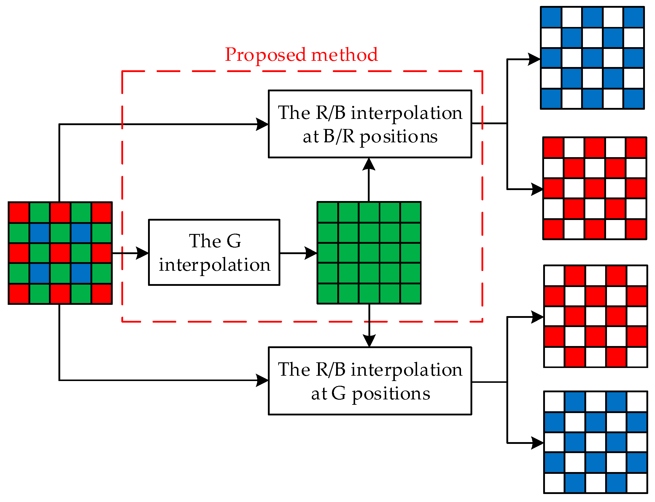
The outline of the proposed algorithm is shown in Figure 4. Firstly, the proposed algorithm recovers the G components by adopting the posteriori idea. Then, the R/B components at G positions are recovered by the same method as in [8]. Finally, the correlation of R–B channels in high frequency is used to recover the missing R/B components at B/R positions. The novel part of the proposed algorithm is marked by a red dotted line in Figure 4.

3.2. The G Interpolation at R/B Positions

It is vital to recover the missing G components because the human eyes are more sensitive to the green color and the number of G pixels are twice that of the R or B pixels. The quality of G interpolation directly affects the final interpolation effect. Therefore, the missing G components are interpolated first. The complete process of G interpolation at R positions (the process of G interpolation at B positions is the same) is shown in Figure 5.
Firstly, the directional estimations G h and G v are calculated by the same method as in ACP [8], as shown in Equation (1) and Equation (2), respectively. The 5 × 5 image block is adopted, as shown in Figure 1. Then, the directional gradients need to be calculated appropriately. This is a crucial step because weights are obtained based on the gradients. Note that it is the most important factor for a successful interpolation algorithm to obtain the weight suitable for the estimation of each direction. The gradients calculated by Equation (3) and Equation (4) are independent of the directional estimations G h and G v , attributing the poor matching between the weights and direction estimations. To make the weights match the estimations better, the correlation between the gradients and estimations needs to be increased. For this reason, the posteriori idea is introduced into the calculation of gradients. To be more specific, we replace the original G values with G h and G v when calculating the gradients. Equation (3) and Equation (4) are modified as follows, respectively:
D h ( i , j ) = | R ( i , j 1 ) R ( i , j + 1 ) | + | 2 G h ( i , j ) G h ( i , j 1 ) G h ( i , j + 1 ) | ,
D v ( i , j ) = | R ( i 1 , j ) R ( i + 1 , j ) | + | 2 G v ( i , j ) G v ( i 1 , j ) G v ( i + 1 , j ) | .
The posteriori gradients in the horizontal and vertical directions, D h and D v , are available now. Next, the weights in the horizontal and vertical directions are calculated. We have the following considerations: (i) Where the gradient is large, the color changes rapidly, and the weight in this direction should be small; where the gradient is small, the color changes slowly and the weight should be large. That is to say, the bigger the gradient is, the smaller the weight in this direction will be, and vice versa. (ii) The neighboring gradient values can be involved to the calculation of weights. Based on the two considerations mentioned above, the weights in the horizontal and vertical directions, W h and W v , are defined as:
W h ( i , j ) = 1 ( a = i 2 i + 2 b = j 2 j + 2 D h ( a , b ) ) 2 ,
W v ( i , j ) = 1 ( a = i 2 i + 2 b = j 2 j + 2 D v ( a , b ) ) 2 ,
where a and b indicate the row and the column in the 5 × 5 image block, respectively. Finally, average the horizontal estimation G h and vertical estimation G v according to different weights. The G interpolation equation is given as follows:
G ( i , j ) = G h ( i , j ) × W h ( i , j ) + G v ( i , j ) × W v ( i , j ) W h ( i , j ) + W v ( i , j ) .
All the G values can be recovered by applying the steps above to the R/B positions.

3.3. The R/B Interpolation at G Positions

After the G components are recovered completely, the R/B components at G positions need to be interpolated. To keep the computational complexity low, we use the same method as in ACP [8]. Considering a 5 × 5 image block centered on the G pixel, the interpolation equations are given as follows [8]:
R ( i , j ) = 1 2 [ R ( i , j 1 ) + R ( i , j + 1 ) ] + 1 4 [ 2 G ( i , j ) G ( i , j 2 ) G ( i , j + 2 ) ] ,
B ( i , j ) = 1 2 [ B ( i 1 , j ) + B ( i + 1 , j ) ] + 1 4 [ 2 G ( i , j ) G ( i 2 , j ) G ( i + 2 , j ) ] .

3.4. The R/B Interpolation at B/R Positions

In this section, a novel method for recovering R/B components at B/R positions is introduced, which is shown in Figure 6. Considering a 5 × 5 image block as shown in Figure 1, the interpolation steps at R 13 pixel are as follows. Note that all the G values and the R/B values at the G positions are available. Firstly, the color differences are redefined in the proposed algorithm. Conventional algorithms [15,16,19,21,22] define the color differences as G R or G B , but we calculate the color differences by R B or B R . Because the correlation between the B components and the R components in high frequency is more than the G components. Menon et al. proved this in [10]. Furthermore, the color differences in the proposed algorithm are calculated along the north (N), south (S), west (W), and east (E) directions rather than the four diagonal directions (NW, NE, SW, and SE), which is different from LDI-NAT [16]. For the reason that a pixel is closer to adjacent pixels in its N, S, W, and E directions than it is in its NW, NE, SW, and SE directions, the correlation in N, S, W, and E directions is greater than in its NW, NE, SW, and SE directions. Therefore, the color differences in the N, S, W, and E directions, d RB N , d RB S , d RB W , and d RB E , are defined as:
d RB N = B 8 R 8 ,
d RB S = B 18 R 18 ,
d RB W = B 12 R 12 ,
d RB E = B 14 R 14 .
Then, the gradients are calculated along the N, S, W, and E directions. We have the following considerations: (i) Both the center pixels and the neighboring pixels need to be used to calculate the gradients. (ii) The central pixels contribute more than the neighboring pixels. (iii) The additional information from the B channel needs to be used for more accurate estimates because of the great correlation existing in R–B channels. Based on the considerations mentioned above, the gradients are defined as:
RB N = | B 8 B 18 | + | R 3 R 13 | + 1 2 | G 2 G 12 | + 1 2 | G 4 G 14 | ,
RB S = | B 8 B 18 | + | R 23 R 13 | + 1 2 | G 22 G 12 | + 1 2 | G 24 G 14 | ,
RB W = | B 12 B 14 | + | R 11 R 13 | + 1 2 | G 16 G 18 | + 1 2 | G 6 G 8 | ,
RB E = | B 12 B 14 | + | R 15 R 13 | + 1 2 | G 10 G 8 | + 1 2 | G 20 G 18 | ,
where RB N , RB S , RB W , and RB E indicate the gradients in the N, S, W, and E directions, respectively. Next, the weights θ X are defined as the reciprocals of gradients, which can be expressed as:
θ X = 1 RB X ,   X ( N , S , W , E ) ,
where θ X indicates the weights in the four directions (N, S, W, and E) at the R 13 pixel.
The color differences and weights in the N, S, W, and E directions are available after the above steps. The final color difference estimation, d RB , can be calculated by combining the color differences with the weights, which can be expressed as:
d RB = θ X × d RB X θ X , X ( N , S , W , E ) .
Finally, the missing B component at the R 13 pixel can be recovered by adding the final color difference estimation d RB to the R 13 pixel value:
B 13 = R 13 + d RB .
The steps to interpolate the R components at the B pixels are the same as above.

4. Experimental Results and Performance Analyses

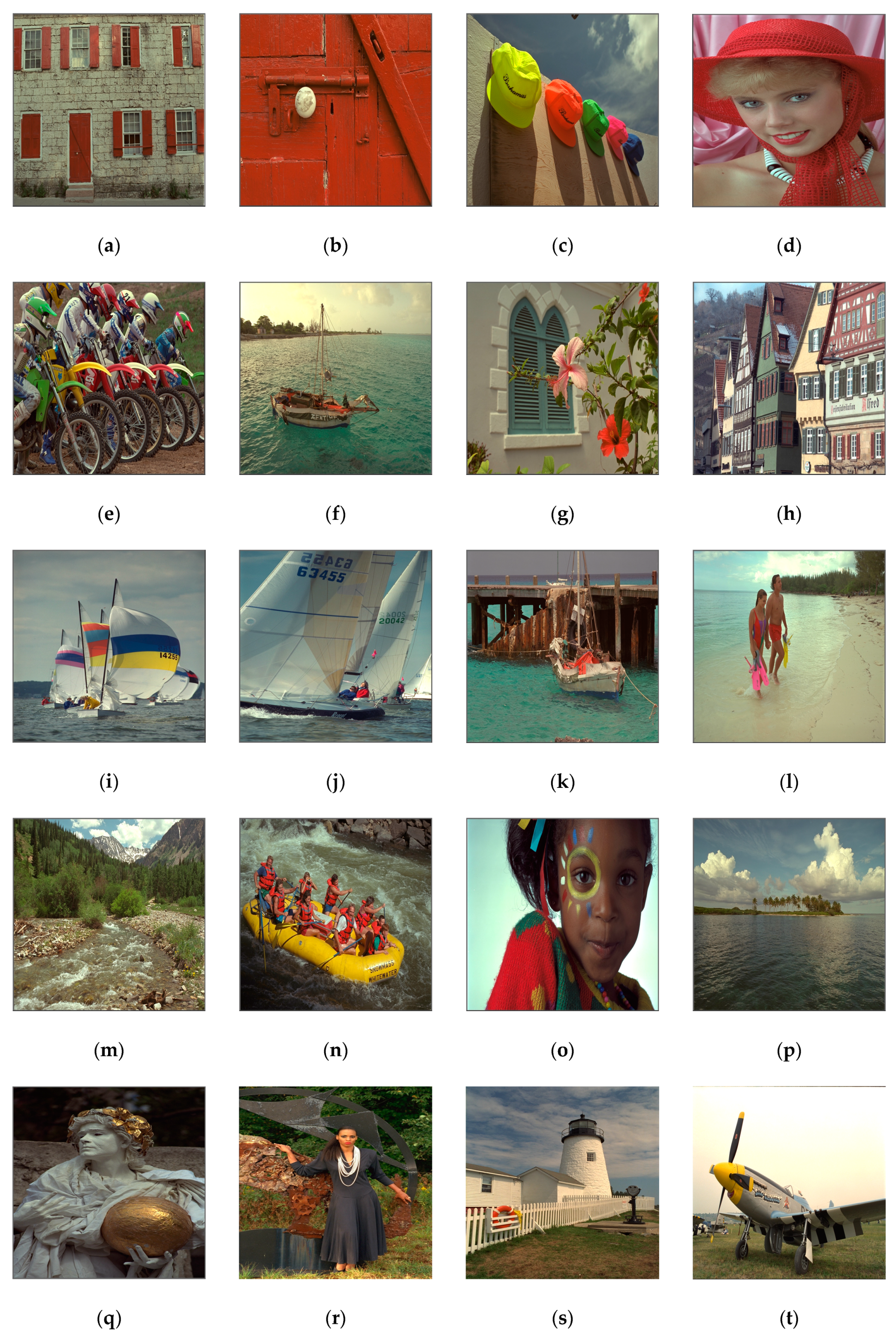
To evaluate the effectiveness of the proposed algorithm in image reconstruction, we used MATLAB R2017b with an Intel Core i7-5500U and 2.40 GHz CPU computer to test the Kodak dataset [29] that contains 24 color images. The 24 color images of the Kodak dataset are shown in Figure 7. Each image is either 768 × 512 or 512 × 768 in size. Note that though all the images in Figure 7 are compressed for display, our experiments still used the original Kodak images.
To evaluate the quality of reconstructed images, we used the composite peak signal-to-noise ratio (CPSNR), which is a commonly used evaluation standard. We compared the proposed algorithm with ACP [8], DWDF [10], DLMMSE [12], RAD [13], IG [14], and LDI-NAT [16]. Compared to the two original algorithms (ACP [8] and LDI-NAT [16]), the proposed algorithm has two improvements. Therefore, the comparisons in the case of with/without each improvement were also needed. The original G interpolation and the original R/B interpolation at the B/R positions (OAO), the improved G interpolation and the original R/B interpolation at B/R positions (IAO), and the original G interpolation and the improved R/B interpolation at B/R positions (OAI) were involved in the evaluation. The results of CPSNR are shown in Table 1. The best result of each image was marked in bold. Two decimal digits were retained.
Additionally, inspired by the work in [25], an ordinary least squares regression analysis that can identify possible errors was performed. To be specific, we performed CPSNR fitting between the proposed algorithm and the other nine algorithms, respectively, and computed the p values ( p ). Experimental results show that all the p values are less than 10 4 . The smaller the p value is, the more convincing the comparisons between the proposed algorithm and the other nine algorithms are.
Furthermore, the structural similarity index (SSIM), as an index to measure the similarity between the reconstructed image and the original image, was also widely applied to evaluate the effectiveness of interpolation algorithms. However, according to the work in [25], the correlation between the CPSNR and SSIM is high. Therefore, there is no reason to calculate the SSIM if the CPSNR is available. Meanwhile, it is beneficial to avoid large tables.
Combining the results in Table 1 and the p values, we have the following analyses. In the results of CPSNR from Table 1, the proposed algorithm had different degrees of improvement of CPSNR in 18 out of 24 images compared to the other nine algorithms. Especially in Figure 7b, the CPSNR of the proposed algorithm was at least 0.86 dB higher than that of the other nine algorithms. Furthermore, the average CPSNR of IAO, OAI, and the proposed algorithm reached 1.64 dB, 0.58 dB, and 1.95 dB higher than that of OAO ( p < 10 4 ), respectively. These results demonstrate that the two improvements have significant effects, especially the combination of the two. The proposed algorithm did not generate the best results in all the 24 images, but the average CPSNR of the proposed algorithm was the highest among the ten algorithms, reaching 0.60 dB and 0.64 dB higher than that of IG [14] and LDI-NAT [16] ( p < 10 4 ), respectively. Furthermore, what is worth mentioning again is that all the p values were less than 10 4 , which demonstrates that the comparisons are convincing. Therefore, the proposed algorithm actually has better performance to reconstruct the full-color images compared to the other nine algorithms.
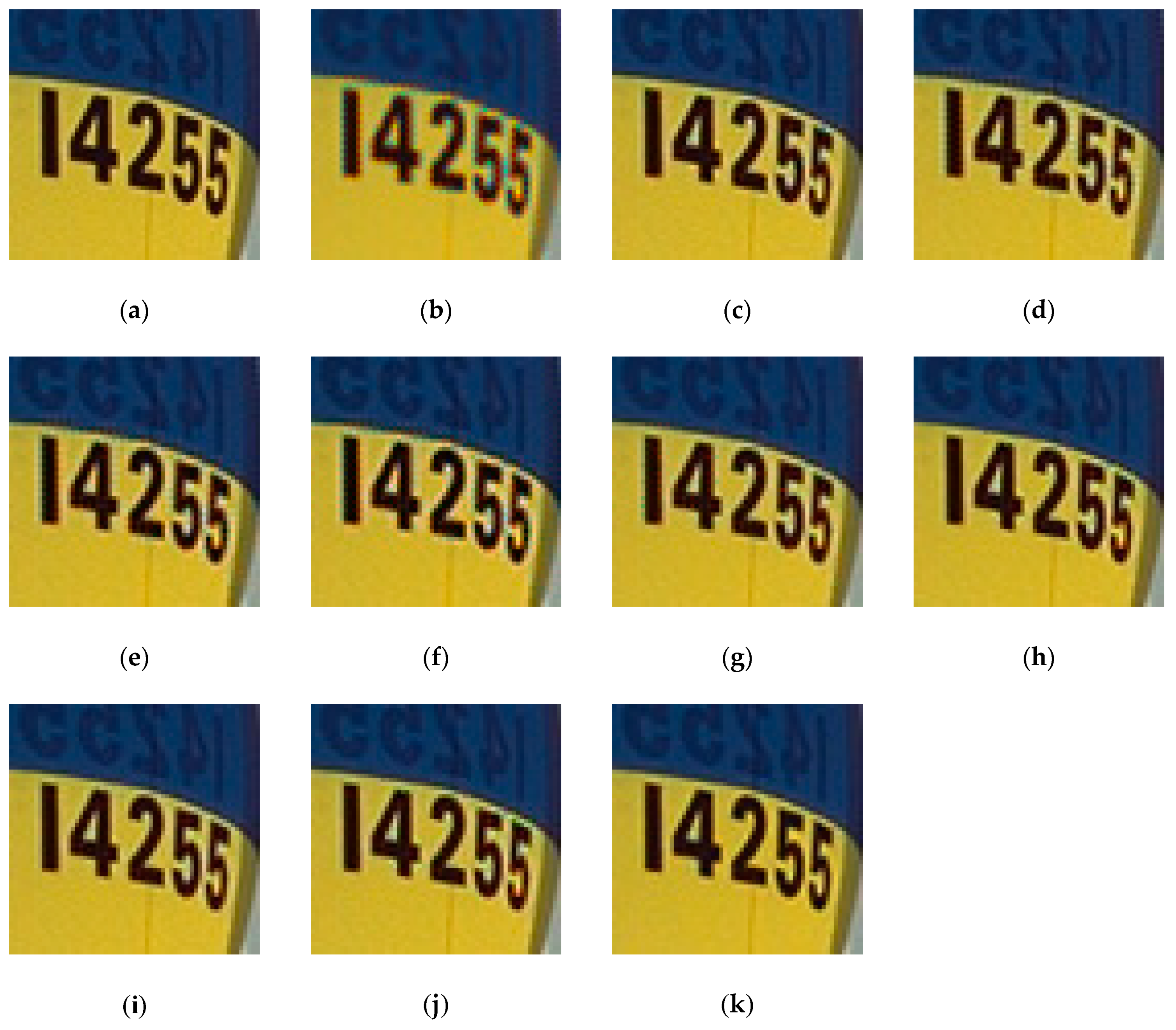
In addition to objective evaluations, visual effect is also an important standard to evaluate the interpolation effectiveness. To show a visual comparison of reconstructed images processed by different algorithms, we reconstructed an image by the ten different algorithms mentioned above. The position in Figure 7i that has been marked by a yellow box in Figure 8 contains many edge regions that are prone to color artifacts and distortions. Therefore, Figure 7i was selected as the test image. Furthermore, we magnified the position of the yellow box in Figure 8 to show the comparisons of visual effect more clearly. The pixels contained in the yellow box are 60 × 60 in size, starting at (385,390). The reconstructed images of the enlarged region of the yellow box processed by the ten different algorithms are shown in Figure 9.
The image processed by the proposed algorithm has slight color artifacts and distortions at the edges of the number part, as shown in Figure 9k, but the color artifacts and distortions are more serious visually in the images processed by the other nine algorithms, as shown in Figure 9b–j. The image processed by the proposed algorithm also preserves more details. The visual comparisons of reconstructed images demonstrate that the proposed algorithm has a better effect in image interpolation when compared to the other nine algorithms, especially in reconstruction of details.

5. Conclusions and Remarks on Possible Future Work

In this paper, we propose a weights-based demosaicking algorithm that applies the posterior idea and the great correlation of R–B channels in high frequency. To reconstruct the G components at the R/B positions, the G values in the horizontal and vertical directions are first estimated. Then, the gradients are calculated by a novel posteriori method in the horizontal and vertical directions. The weights are obtained based on the posterior gradients in the horizontal and vertical directions. Finally, the weights and G estimations are combined to generate the full G image. After interpolating the R/B components at the G positions by the same method as in ACP [8], another novel weights-based method is applied to recover the missing R/B components at the B/R positions. Firstly, the color differences are calculated in the N, S, W, and E directions by using the great correlation of R–B channels in high frequency. Then, additional B/R channel information is added to the calculation of gradients. The weights are obtained based on the gradients. Finally, the weights and color differences are combined to generate the final color difference estimations that are added to the B/R pixel values to recover the missing R/B components at the B/R positions. Experimental results show that our algorithm performs well not only in the objective experimental measurement but also in the subjective visual effect.
However, the R/B interpolation at the G position is still processed in one direction, which will negatively affect the interpolation effect. Therefore, we will focus on how to improve the R/B interpolation effect at the G positions in the future work.

Author Contributions

M.X., C.W., and W.G. conceived the algorithm and designed the experiments; M.X. and W.G. performed the experiments; M.X., C.W., and W.G. analyzed the results; W.G. drew the block diagrams; M.X. and W.G. drafted the manuscript; M.X., C.W., and W.G. revised the manuscript. C.W. supervised the project. All authors read and approved the final manuscript.

Funding

This work was supported by the National Natural Science Foundation of China (No. 61702303); the Shandong Provincial Natural Science Foundation, China (No. ZR2017MF020); the 13th student research training program (SRTP) at Shandong University (Weihai), China; and the 10th undergraduate research apprentice program (URAP) at Shandong University (Weihai), China.

Acknowledgments

The authors thank Shiyue Chen, Ran Liu, Xinghong Hu, Wenjie Wu, Yusen Zhang, and Zihan Wang for their help in revising this paper.

Conflicts of Interest

The authors declare no conflict of interest.

References

  1. Menon, D.; Calvagno, G. Color image demosaicking: An overview. Signal Process. Image Commun. 2011, 26, 518–533. [Google Scholar] [CrossRef]
  2. Bayer, B.E. Color imaging array. U.S. Patent 3,971,065, 20 July 1976. [Google Scholar]
  3. Longere, P.; Zhang, X.M.; Delahunt, P.B.; Brainard, D.H. Perceptual assessment of demosaicing algorithm performance. Proc. IEEE 2002, 90, 123–132. [Google Scholar] [CrossRef] [Green Version]
  4. Malvar, H.S.; He, L.W.; Cutler, R. High-quality linear interpolation for demosaicing of Bayer-patterned color images. In Proceedings of the IEEE International Conference on Acoustics, Speech, and Signal Processing, Montreal, QC, Canada, 17–21 May 2004; pp. 485–488. [Google Scholar]
  5. Luo, X.; Sun, H.J.; Chen, Q.P.; Chen, J.; Wang, Y.J. Real-time demosaicing of Bayer pattern images. Chin. J. Opt. Appl. Opt. 2010, 3, 182–187. [Google Scholar]
  6. Wang, D.Y.; Yu, G.; Zhou, X.; Wang, C.Y. Image demosaicking for Bayer-patterned CFA images using improved linear interpolation. In Proceedings of the 7th International Conference on Information Science and Technology, Da Nang, Vietnam, 16–19 April 2017; pp. 464–469. [Google Scholar]
  7. Zhou, X.; Yu, G.; Yu, K.; Wang, C.Y. An effective image demosaicking algorithm with correlation among Red-Green-Blue channels. Int. J. Eng. Trans. B 2017, 30, 1190–1196. [Google Scholar]
  8. Adams, J.E.; Hamilton, J.F. Adaptive color plan interpolation in single sensor color electronic camera. U.S. Patent 5,629,734, 13 May 1997. [Google Scholar]
  9. Lee, J.; Jeong, T.; Lee, C. Improved edge-adaptive demosaicking method for artifact suppression around line edges. In Proceedings of the Digest of Technical Papers International Conference on Consumer Electronics, Las Vegas, NV, USA, 10–14 January 2007; pp. 1–2. [Google Scholar]
  10. Menon, D.; Andriani, S.; Calvagno, G. Demosaicing with directional filtering and a posteriori decision. IEEE Trans. Image Process. 2007, 16, 132–141. [Google Scholar] [CrossRef] [PubMed]
  11. Chen, W.J.; Chang, P.Y. Effective demosaicking algorithm based on edge property for color filter arrays. Digit. Signal Process. 2012, 22, 163–169. [Google Scholar] [CrossRef]
  12. Zhang, L.; Wu, X.L. Color demosaicking via directional linear minimum mean square-error estimation. IEEE Trans. Image Process. 2005, 14, 2167–2178. [Google Scholar] [CrossRef] [PubMed] [Green Version]
  13. Shi, J.; Wang, C.Y.; Zhang, S.Y. Region-adaptive demosaicking with weighted values of multidirectional information. J. Commun. 2014, 9, 930–936. [Google Scholar] [CrossRef]
  14. Chung, K.H.; Chan, Y.H. Low-complexity color demosaicing algorithm based on integrated gradients. J. Electron. Imaging 2010, 19, 021104. [Google Scholar] [CrossRef] [Green Version]
  15. Pekkucuksen, I.; Altunbasak, Y. Gradient based threshold free color filter array interpolation. In Proceedings of the 17th IEEE International Conference on Image Processing, Hong Kong, China, 26–29 September 2010; pp. 137–140. [Google Scholar]
  16. Zhang, L.; Wu, X.L.; Buades, A.; Li, X. Color demosaicking by local directional interpolation and nonlocal adaptive thresholding. J. Electron. Imaging 2011, 20, 023016. [Google Scholar] [Green Version]
  17. Chen, X.D.; Jeon, G.; Jeong, J. Voting-based directional interpolation method and its application to still color image demosaicking. IEEE Trans. Circuits Syst. Video Technol. 2014, 24, 255–262. [Google Scholar] [CrossRef]
  18. Wu, J.J.; Anisetti, M.; Wu, W.; Damiani, E.; Jeon, G. Bayer demosaicking with polynomial interpolation. IEEE Trans. Image Process. 2016, 25, 5369–5382. [Google Scholar] [CrossRef] [PubMed]
  19. Kiku, D.; Monno, Y.; Tanaka, M.; Okutomi, M. Residual interpolation for color image demosaicking. In Proceedings of the 20th IEEE International Conference on Image Processing, Melbourne, VIC, Australia, 15–18 September 2013; pp. 2304–2308. [Google Scholar]
  20. He, K.M.; Sun, J.; Tang, X.Q. Guided image filtering. IEEE Trans. Pattern Anal. Mach. Intell. 2013, 35, 1397–1409. [Google Scholar] [CrossRef] [PubMed]
  21. Kiku, D.; Monno, Y.; Tanaka, M.; Okutomi, M. Minimized-Laplacian residual interpolation for color image demosaicking. In Proceedings of the SPIE-IS and T Electronic Imaging - Digital Photography X, San Francisco, CA, USA, 3–5 February 2014; pp. 1–8. [Google Scholar]
  22. Yu, K.; Wang, C.Y.; Yang, S.; Lu, Z.W.; Zhao, D. An effective directional residual interpolation algorithm for color image demosaicking. Appl. Sci. 2018, 8, 680. [Google Scholar] [CrossRef]
  23. Wang, L.; Jeon, G. Bayer pattern CFA demosaicking based on multi-directional weighted interpolation and guided filter. IEEE Signal Process. Lett. 2015, 22, 2083–2087. [Google Scholar] [CrossRef]
  24. Monno, Y.; Kiku, D.; Tanaka, M.; Okutomi, M. Adaptive residual interpolation for color and multispectral image demosaicking. Sensors 2017, 17, 2787. [Google Scholar] [CrossRef] [PubMed]
  25. Thomas, J.B.; Farup, I. Demosaicing of periodic and random color filter arrays by linear anisotropic diffusion. J. Imaging Sci. Technol. 2018, 62, 050401. [Google Scholar] [CrossRef]
  26. Zhang, L.; Lukac, R.; Wu, X.L.; Zhang, D. PCA-based spatially adaptive denoising of CFA images for single-sensor digital cameras. IEEE Trans. Image Process. 2009, 18, 797–812. [Google Scholar] [CrossRef] [PubMed]
  27. Djeddi, M.; Ouahabi, A.; Batatia, H.; Basarab, A.; Kouamé, D. Discrete wavelet for multifractal texture classification: Application to medical ultrasound imaging. In Proceedings of the 17th IEEE International Conference on Image Processing, Hong Kong, China, 26–29 September 2010; pp. 637–640. [Google Scholar]
  28. Ahmed, S.S.; Messali, Z.; Ouahabi, A.; Trepout, S.; Messaoudi, C.; Marco, S. Nonparametric denoising methods based on Contourlet transform with sharp frequency localization: Application to low exposure time electron microscopy images. Entropy 2015, 17, 3461–3478. [Google Scholar] [CrossRef]
  29. Eastman Kodak Company. Kodak lossless true color image suite—Photo CD PCD0992. Available online: http://r0k.us/graphics/kodak/index.html (accessed on 25 April 2019).
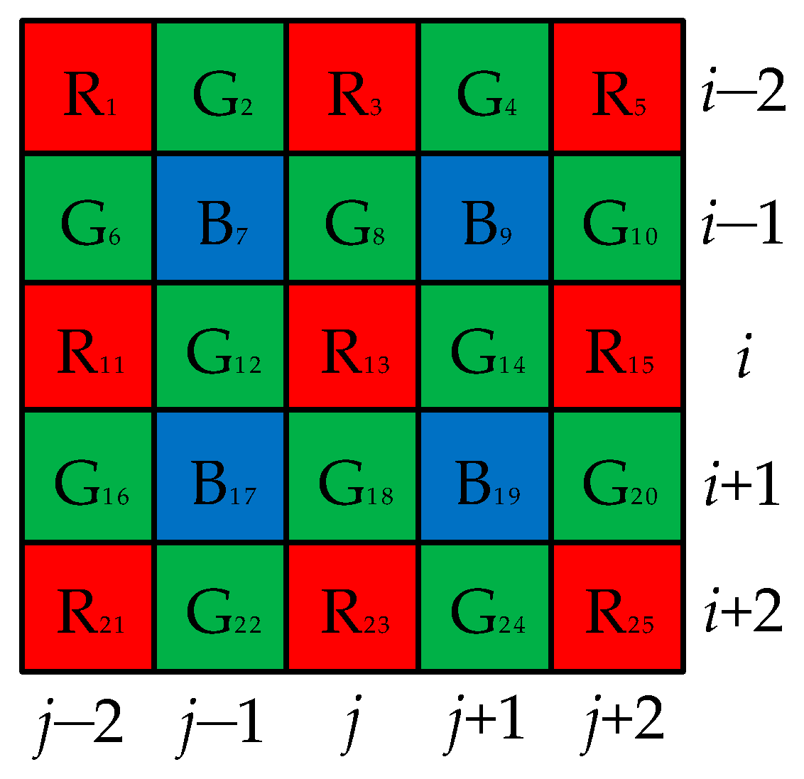
Figure 1. Color filter array (Bayer pattern).
Symmetry 11 00600 g001
Figure 2. The outline of G interpolation in ACP.
Symmetry 11 00600 g002
Figure 3. The process of B interpolation at R positions in LDI-NAT.
Symmetry 11 00600 g003
Figure 4. The outline of the proposed algorithm.
Symmetry 11 00600 g004
Figure 5. The process of G interpolation at R positions using the proposed algorithm.
Symmetry 11 00600 g005
Figure 6. The B interpolation at the R position in the proposed algorithm.
Symmetry 11 00600 g006
Figure 7. Kodak dataset.
Symmetry 11 00600 g007aSymmetry 11 00600 g007b
Figure 8. The original image marked by a yellow box.
Symmetry 11 00600 g008
Figure 9. Visual comparison of reconstructed images: (a) the enlarged region of the yellow box; (b) reconstructed by ACP; (c) reconstructed by DWDF; (d) reconstructed by DLMMSE; (e) reconstructed by RAD; (f) reconstructed by IG; (g) reconstructed by LDI-NAT; (h) reconstructed by OAO; (i) reconstructed by IAO; (j) reconstructed by OAI; (k) reconstructed by the proposed algorithm.
Symmetry 11 00600 g009
Table 1. The CPSNR (dB) of the Kodak images.
ImagesACP
[8]
DWDF
[10]
DLMMSE
[12]
RAD
[13]
IG
[14]
LDI-NAT
[16]
OAOIAOOAIProposed
Figure 7a34.0235.2734.9834.3635.4435.8234.0736.2134.6536.51
Figure 7b38.9340.2238.5738.8337.2140.1938.9440.3839.7841.24
Figure 7c39.2641.6640.1239.2341.5141.4840.4541.8141.1441.85
Figure 7d38.7639.8737.9038.2938.9040.1739.0440.4439.6640.83
Figure 7e34.1736.1436.9834.6936.2737.0034.9737.0235.3737.08
Figure 7f33.8637.5636.1533.9937.1436.2735.2037.3935.9837.63
Figure 7g41.5341.1440.6640.8640.8841.4540.3041.2741.0541.94
Figure 7h32.1033.8133.2931.7833.8533.8232.4133.5433.0033.69
Figure 7i41.9341.3141.9340.5241.4740.7539.1640.5439.6442.08
Figure 7j41.1941.0640.8640.8741.3841.1639.4541.4440.2341.95
Figure 7k35.5637.9836.0535.8338.0037.9836.2638.3937.0738.75
Figure 7l40.5542.2239.9838.9941.5741.0840.3642.1141.4242.55
Figure 7m30.4131.6431.3731.2032.0932.0330.4932.6230.9632.70
Figure 7n35.6236.3437.1035.5636.7537.1435.8436.9836.1337.00
Figure 7o36.8738.8235.9536.2238.4338.8637.5039.3438.2039.42
Figure 7p39.2141.4840.8938.6440.7939.2438.5041.0239.3141.04
Figure 7q37.8539.7039.6838.5041.1439.9238.5440.0539.1340.06
Figure 7r34.4734.7134.2035.1435.5535.2933.8635.7834.2235.81
Figure 7s37.7138.1338.1737.5138.5838.1536.7838.7137.4138.82
Figure 7t37.1237.9537.8137.1038.9939.2837.8639.2738.4339.66
Figure 7u34.6236.4334.6935.0037.0237.0835.5737.4636.0337.71
Figure 7v35.7136.6536.1236.0437.8937.5436.2737.6736.7938.08
Figure 7w39.8640.8740.5239.3242.6242.3341.4541.5940.9841.61
Figure 7x31.5430.0632.3932.5234.2133.1631.9833.7532.5833.81
Average36.7937.9637.5636.7138.2438.2036.8938.5337.4738.84