Multi-Phase and Integrated Multi-Objective Cyclic Operating Room Scheduling Based on an Improved NSGA-II Approach

Abstract

The operating room (OR) is an important department in a hospital, and the scheduling of surgeries in ORs is a challenging combinatorial optimization problem. In this paper, we address the problem of multiple resource allocation of ORs and propose a surgery scheduling scheme for OR units. To solve this problem, a multi-phase and integrated multi-objective linear programming model is proposed. The first phase of the proposed model is a resource allocation model, which mainly focuses on the allocation of ORs for each surgical specialty (SS). Based on the results of the first phase, the second phase is the cyclic Master Surgical Schedule model, which aims to schedule the surgeries in each SS. The proposed models are solved by the Non-dominated Sorting Genetic Algorithm II (NSGA-II), which was improved. Finally, two numerical experiments based on practical data are provided to verify the effectiveness of the proposed models as well as to evaluate the performance of the improved NSGA-II. Our final results illustrate that our proposed model can provide hospital managers with a series of “optimal” solutions to effectively allocate relevant resources and ORs for surgeries, and they show that the improved NSGA-II has high computational efficiency and is more suitable in solving larger-scale problems.

1. Introduction

Operating room (OR) scheduling is a notoriously intricate and diverse process, considering the involved content and amount of resources [1]. This includes a determination of the operation time and optimization of the allocation of various operation resources required by the ORs and various surgical specialties (SSs) in order to complete the whole operation process. Hospital managers usually try to meet conflicting goals, such as OR utilization, efficiency, patients’ waiting times, the quality of treatment, and labor, realizing that making everything satisfying is difficult and even impossible sometimes. This can explain why patients waiting, uneven utilization, and operations delays often occur in ORs. Therefore, the OR optimization of a hospital is an urgent problem for hospital administrators to solve [2]. Most OR scheduling decisions are simple strategies based on qualitative approaches [3,4], while more and more researchers have paid an interest to quantitative approaches during the past decades. Among them, mathematical models and methods for operations research are most commonly used [4]. Below, we introduce some of the key characteristics of OR planning and scheduling problems.

For different surgeries, the types of surgery can be generally divided into three types: elective, emergency, and urgent [5]. Emergency surgeries usually need to be carried out within two hours of going to the hospital, and they need to be carried out immediately. Elective surgeries can be arranged in advance.

In addition, OR scheduling methods can be divided into block scheduling and open scheduling [6]. Block scheduling means that OR time is expressed in a block way. Usually half a day or one day of an OR is represented as a block to be allocated to the required SS, and open scheduling is mainly based on the needs of surgeons for OR time. Over the years of research experience by scholars, it has been found that block scheduling can not only arrange OR scheduling more reasonably, but can also let surgeons know the surgical time in advance. It can also improve the efficiency of OR scheduling. Block scheduling can be divided into three main phases.

The first phase is primarily a time planning problem (TPP). The problem is the allocation of OR time between SSs based on the availability of OR resources. The distribution process can be based on historically similar OR costs, income, and OR utilization. This phase is called "advance scheduling" in the literature [7]. Blake and Carter [8] proposed a mathematical model based on two linear programming methods in order to enable a hospital to break even, while ensuring the surgeon’s income and minimizing the impact of these external factors on the ORs. Dexter et al. [9] addressed the economic impact of OR scheduling by combining relevant financial indicators and the uncertainty of the workload in the ward.

When an OR time is assigned to each SS in the first phase, the second phase is mainly based on the results of the first phase of the master surgical schedule (MSS), in which the elective patients must be scheduled in each assigned OR. At present, research results on MSS are quite rich, and the focus of this attention is different. There is much research that has focused on OR utilization, OR openings, overtime and idle time costs, patient waiting times, and patient and medical staff preferences. Guinet and Chaabane [10] turned the MSS problem into a generalized surgical assignment problem in order to reduce patient waiting times and overtime in ORs. Ozkarahan [11] solved a surgical problem among multiple ORs, the optimization goal of which was unused and over-utilized OR resources: This mainly used the goal planning method. We have observed that some research still treats multi-objective as a single one in OR scheduling issues even if the importance of considering multiple conflicting goals has already been realized. Actually, multi-objective mathematical programming models have been considered by lots of authors (e.g., [12,13,14,15]), while most solution approaches have been almost on a single objective. For example, some have given each objective a weight (the objective program approach [16]), and some have approached the issue using boundary objective functions and hierarchical solving methods [17], which combine objective functions into a single one. We find that the disadvantage is that there exists a dependency on the objective function when the user decides to assign a weighting factor. Thus, we should know about relative importance before combining all of the objectives into one. In addition, users can change the weights used to define several solutions. The third phase is mainly based on the second phase of an MSS: The goal is to determine the optimal sequence for surgical cases. The two phases are referred to as “allocation scheduling” [7]. More works considering both advance and allocation scheduling can be found in References [18,19,20,21,22,23,24,25,26,27,28,29,30,31,32,33].

Although much attention has already been paid to OR scheduling problems, we also have found some open issues: For patients, it is important to reduce patient waiting time and to schedule as many surgeries as possible during the planning period to improve patient satisfaction. However, although most researchers are aware of the seriousness of this problem, they mainly have focused on the time a patient waits for surgery on the day of surgery [34], and we should be aware of optimizing the waiting time for all patients: Increasing surgeries and the number of scheduled surgeries is crucial. For hospital administrators, improving the utilization rate of ORs and maintaining a balanced working time is also a problem worthy of study to increase hospital income and improve the satisfaction of medical staff. In addition, when solving such problems, many of the optimization models that have been established have single objectives, but some papers have applied multi-objective optimization methods, such as References [35,36].

In order to solve the challenges presented above, this paper considers conflicting objectives such as patients, hospital SSs, and ORs to conduct our research. Then, we used a multiphase OR scheduling method and established a multi-objective integer programming model to specify appropriate decisions for hospital OR scheduling. Pareto solutions ensure that standards cannot be improved without deteriorating other standards. Therefore, we propose an improved genetic algorithm approach to find a non-dominant Pareto solution in a reasonable time. As far as we know, (1) some papers have involved multiple decision-making levels, but (2) only one paper [37] has constructed a Pareto boundary through a genetic algorithm.

The remaining part of the paper is as follows. In Section 2, we present a multi-phase and multi-objective integer linear programming model (MILPM). In Section 3, we introduce two approaches to solve the proposed models in detail. In Section 4, two numerical experiments based on practical data and comparison discussion are provided. Finally, in Section 5, a conclusion completes and sums up the paper.

2. Multiphase and Integrated Multi-Objective Linear Programming Model

When scheduling for multiple SSs and multiple ORs, decision-makers find it difficult to know in advance how to allocate OR time to SSs and arrange surgeries once OR time is allocated to SSs. It is not a simple problem to allocate OR time to SSs because of the following reasons: (1) An allocation to an SS may not be exactly the scattered time period it needs, but an entire OR block, and it is not necessarily assigned to the specified block; and (2) the time allocated to SSs may be affected by the availability of resources and professional equipment in the ORs.

Thus, due to the reasons above, the procedure of OR scheduling is very complicated. In this process, not only should ORs, patients, and other factors be considered, but also the constraints of OR resources should be comprehensively considered. Therefore, the problem of OR scheduling can be transformed into multi-constraint and multi-objective optimizing problems. According to a more effective idea, hospital OR scheduling is divided into two phases: The first phase is an OR resource allocation model. The goal is to optimize the allocation of OR resources to each SS during the planning period. The second phase is the master surgical schedule model. Based on the OR time having been allocated to SSs in the previous phase, the specific surgery schedule of each SS is worked out.

2.1. Problem Description

The main problem to be solved in our paper is the allocation of ORs between different SSs belonging to the same hospital department, and then the surgical arrangements within a single SS. In the surgical department of a hospital, there is a Surgery Management Center (SMC) that arranges surgeries for the entire department. In a scheduling period (this paper considers three days), each SS has a patient waiting list. This list can include new arrivals and unscheduled surgeries from the last period, and this paper only considers elective surgery. Before the start of the period, the SS reports the surgical information to be performed to the SMC for the next three days. The information about the surgeries mainly includes patients’ personal information, examination statuses, and deadlines for the surgeries. The SMC assigns each SS to available ORs for the next period according to the report information of the patient waiting list for each SS, and then each SS arranges the OR and surgical time for each patient according to the urgency of the patient’s condition (the deadline of the surgery), according to the available ORs.

As with most papers in this field, in order to apply the method proposed in this paper to a real hospital scene, the paper made the following assumptions before the modeling: (a) The surgery time is transformed into the number of ORs to be allocated; (b) this paper considers the use of mixed public ORs, all of which are of the same grade; (c) the requirements for the surgery to be performed in each SS are at the same phase of health requirements or lower for the phase of hygiene; (d) the duration of the surgery in this paper includes preoperative and postoperative time; (e) the ORs are fully resourced before the surgery begins; (f) in this paper, we mainly consider elective surgeries (in hospitals, extra ORs are usually reserved to arrange for emergencies and outpatients); (g) doctors can predict the length of surgery and the time of the latest surgery according to the patient’s condition; and (h) before the start of surgery (i.e., when the patient is admitted to the hospital), the doctor judges the patient’s latest operation time based on disease type characteristics and an examination report of the initial patient, so in order to treat the patient in time, each patient must be operated on before the latest deadline.

2.2. Operating Room Resource Allocation Model (Phase 1)

The Operating Room Resource Allocation Model is formulated based on the following rule: For an OR department in a hospital, each SS reports specific information about patients to the SMC in a period. The SMC allocates ORs to each SS according to the surgical time required by each SS.

When establishing the model, we first designed the problem notations used in the model, which are described in

Table 1. Problem notations in Phase 1. OR: operating room; SS: surgical specialty.

Symbol	Description
M	set of surgical specialties
m	index for surgical specialties in M
T	scheduling period
K	set of ORs
H	normal open hours per OR per day
Maxk	maximum overtime allowed per day per OR
RT	total time required by each SS during the scheduling period
rtm	time required by the SS m during the scheduling period
profitm	surgical benefit per unit time of the SS m
costm	the overtime cost of the SS m
allocm	the number of ORs assigned to the SS m
Minm	the minimum OR time requirement for the SS m during the scheduling period

.

The formulation of the model and notations are as follows.

The objective function $optf\left(x\right)=\left[f_1\left(x\right),f_2\left(x\right)\right]$ is

$$\max {\displaystyle \sum _{m=1}^{M}profi{t}_{m}r{t}_m},$$

(1)

$$\min {\displaystyle \sum _{m=1}^M\left(r{t}_m-H\ast allo{c}_m\ast T\right)\cos t_m},$$

(2)

Subject to

$${\displaystyle \sum _{m=1}^M}H\ast allo{c}_m\ast T\le \left(H+Ma{x}_k\right)\ast K\ast T\forall m,m=1,2,\dots ,M,$$

(3)

$${\displaystyle \sum _{m=1}^{M}allo{c}_m}\le K,$$

(4)

$$allo{c}_m\ge 1\forall m,m=1,2,\dots ,M,$$

(5)

$$H\ast allo{c}_m\ast T\ge Mi{n}_m,\forall m,m=1,2,\cdots ,M.$$

(6)

The objective function Equation (1) maximizes the income of each SS, and the function in Equation (2) aims to minimize the overtime cost when the allocated time cannot meet the demand of the SS. The constraint in Equation (3) is that the total OR time allocated to each SS cannot exceed the total open time of the ORs. The constraint in Equation (4) ensures that the total ORs allocated to SSs cannot exceed the ORs provided. The constraint in Equation (5) means that at least one OR should be allocated to each SS. The constraint in Equation (6) is that the total OR time allocated to each SS must meet the minimum requirements.

2.3. Multiobjective Cyclic Master Surgery Schedule (MSS) Model (Phase 2)

After the first phase has been assigned (ORs to each SS), the results of the first phase are taken as the maximum resource limit when scheduling the patient waiting list for each SS in the second phase.

The cyclic schedule method is used in the industry to arrange the surgeries for SSs among ORs, and is a kind of dynamic scheduling method. This refers to the way in which production scheduling is carried out dynamically in one time period after another as the schedule optimization time goes by. Cyclic scheduling can be carried out either on the basis of the original static scheduling or directly, and the ultimate goal is to get optimal or suboptimal scheduling within the current optimization area.

On the basis of the above assumptions, the specific process of the cyclic schedule is as follows:

Step 1. Because only elective surgeries are considered here, the SSs in a hospital get all of the surgeries that need to be conducted in the next period (three days), and the surgeons mark the patients’ deadlines for the surgeries and the standard duration of the surgeries through patient severity and the results of the examinations (so that the initial surgery pool-L₁ in the schedule is obtained).

Step 2. First of all, the scheme needs to pick out the surgeries from the initial surgery pool-L₁ on the first day and then arrange a suitable OR and surgical sequence for them. The process uses an integrated multi-objective model with four specific indicators selected: (1) the number of surgeries arranged every day, (2) the total OR overtime, (3) the total OR idle time, and (4) the equilibrium rate between ORs in order to select the surgeries and make the specific surgery schedule.

Before establishing the model, the notations used in the model were obtained (described in

Table 2. Problem notations in Phase 2.

Symbol	Description
Im	set of surgeries in SS m
im	index for surgery in Im
K	set of ORs
k	index for OR in K
Nk	the number of surgeries scheduled in OR k
nk	the nth surgery in OR k
$tim{e}_i^m$	the duration of surgery im
$d{d}_i^m$	the deadline of surgery im
Tnormal	the normal working hours in the OR
Topenk	the open hours in OR k for one day
Tover	the overtime in all ORs during the day
Toverk	the overtime of OR k
Num	the total number of surgeries scheduled during the day

). The decision variables are defined as follows:

$$arrang{e}_{i^{m}k{n}^k}=\{\begin{array}{ll}1& \mathrm{if}\mathrm{surgery}{i}^m\mathrm{is}\mathrm{selected}\mathrm{and}\mathrm{arranged}\mathrm{in}\mathrm{the}n\mathrm{th}\mathrm{order}\mathrm{in}\mathrm{OR}k\\ 0& \mathrm{Otherwise}\end{array}.$$

The mathematic model is described as follows:

Objective function $optf\left(x\right)=\left[f_1\left(x\right),f_2\left(x\right),f_3\left(x\right)\right]$ is

$$\max {\displaystyle \sum _{i^m=1}^{I^m}{\displaystyle \sum _{k=1}^K{\displaystyle \sum _{n^k=1}^{N^k}arrang{e}_{i^{m}k{n}^k}}}},$$

(7)

$$\min \left|\left({\displaystyle \sum _{i^m=1}^{I^m}{\displaystyle \sum _{k=1}^K{\displaystyle \sum _{n^k=1}^{N^k}arrang{e}_{i^{m}k{n}^k}tim{e}_i^m-T_{normal}}}}\right)\right|,$$

(8)

$$\min {\displaystyle \sum _{k=1}^K\left|\left({\displaystyle \sum _{i^m=1}^{I^m}arrang{e}_{i^{m}k{n}^k}tim{e}_i^m-\frac{{\displaystyle \sum _{i^m=1}^{I^m}arrang{e}_{i^{m}k{n}^k}tim{e}_i^m}}{K}}\right)\right|},$$

(9)

Subject to

$$variabl{e}_{i^m}=\{\begin{array}{ll}1& whend{d}_i^m\le 1\\ 0& whend{d}_i^m>1\end{array}\forall i^m,i^m=1,2,\dots ,I^m,$$

(10)

$${\displaystyle \sum _{k=1}^K{\displaystyle \sum _{n^k=1}^{N^k}arrang{e}_{i^{m}k{n}^k}\ge variabl{e}_{i^m}}}\forall i^m,i^m=1,2,\dots ,I^m,$$

(11)

$${\displaystyle \sum _{k=1}^K{\displaystyle \sum _{n^k=1}^{N^k}arrang{e}_{i^{m}k{n}^k}\le 1}}\forall i^m,i^m=1,2,\dots ,I^m,$$

(12)

$${\displaystyle \sum _{i^m=1}^{I^m}{\displaystyle \sum _{n^k=1}^{N^k}arrang{e}_{i^{m}k{n}^k}\ast tim{e}_i^m}}\le Tope{n}_k+Tove{r}_k\forall k,k=1,2,\dots ,K,$$

(13)

$${\displaystyle \sum _{i^m=1}^{I^m}arrang{e}_{i^{m}k{n}^k}\le 1}\forall k,k=1,2,\dots ,K\forall n^k,n^k=1,2,\dots ,N^k,$$

(14)

$${\displaystyle \sum _{i^m=1}^{I^m}arrang{e}_{i^{m}k\left(n^k+1\right)}\le {\displaystyle \sum _{i^m=1}^{I^m}arrang{e}_{i^{m}k{n}^k}}}\forall k,k=1,2,\dots ,K\forall n^k,n^k=1,2,\dots ,N^k.$$

(15)

The first objective function, Equation (7), aims to maximize the number of scheduled patients in all ORs in a certain SS, and the second one, Equation (8), minimizes underutilization and overall overtime cost in the OR. The third one, Equation (9), aims for a balance between the ORs according to the standard deviation of the OR working time. The constraint in Equation (10) is the 0–1 variable. It seems that when the deadline is more than 1 day, $variabl{e}_{i^m}$ equals 0: Otherwise, it is 1. The constraint in Equation (11) means that when the deadline for the surgery (latest completion time) is 1 day, the surgery must be completed on the same day. The constraint in Equation (12) prevents the surgery from being repeatedly arranged within the ORs. The constraint in Equation (13) indicates that the total time of the surgeries scheduled in an OR cannot exceed the maximum OR open time. The constraint in Equation (14) ensures that at most one surgery can be performed in one OR in the same period of time. The constraint in Equation (15) assures that the next surgery can be performed only after the current one has been completed in an OR.

Step 3. When surgeries are scheduled on the first day, they are removed from the surgery pool-L₁, and the deadlines for unscheduled surgeries are reduced by one day, $d{d}_i^m=d{d}_i^m-1$. The unselected surgeries form a new surgery pool-L₂. The next two days in the period cycle through the above steps. Through the above three steps in the daily cycle, one can get a cyclic master surgery schedule.

3. Solution Approaches

For a mathematical programming model with multi-objectives, a general purpose model with a wide range of applications is shown below:

$$\max F(x)s.t.G(x)\le 0,H\left(x\right)=0,$$

(16)

where x represents decision variables that are vectors, and a vector with k objective functions forms $F\left(x\right)={\left[f_1\left(x\right),f_2\left(x\right),f_3\left(x\right),\dots ,f_k\left(x\right)\right]}^{\prime }$. Finally, for constraints, G(x) denotes inequalities, and H(x) denotes equality.

The solutions for multi-objective models are very broad. We conduct two approaches here to solve the models: the Goal Programming Approach (GPA) with ILOG CPLEX and the improved Non-dominated Sorting Genetic Algorithm II (NSGA-II) with MATLAB.

3.1. Goal Programming Approach (GPA)

When using the GPA to solve a multi-objective model, we must optimize the high-priority objectives first and then optimize the low-priority objectives. Thus, the Analytic Hierarchy Process (AHP) is proposed to determine the priority of the objectives.

3.1.1. Determining the Priority of the Objectives via AHP

AHP is a decision approach that decomposes decision-making elements into goals, criteria, and programs. On this basis, qualitative and quantitative analysis methods are used. The implementation of AHP is mainly divided into three steps: (1) build a hierarchical model, (2) construct a judgment matrix and calculate the weights of the four objectives, and (3) test the consistency of the judgment matrix.

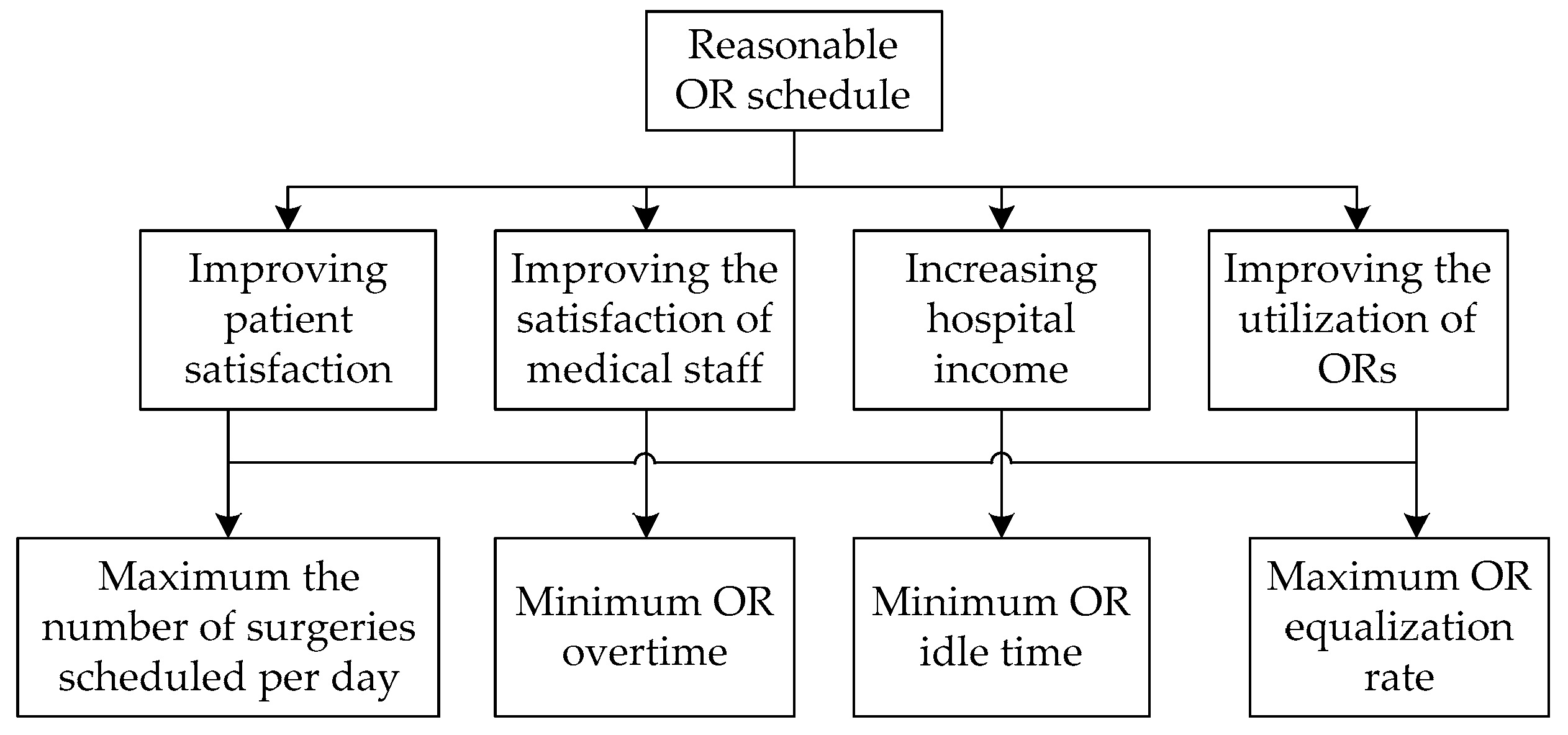
First, by dividing the decision objectives, the factors considered, and the decision objects into the objective layer, the standard layer, and the decision layer according to the mutual relationship between them, the hierarchical structure diagram is drawn (Figure 1). In this section, minimizing overtime and idle time should be considered separately, and the three objectives can be divided into four.

Second, the most important step is to construct a comparison judgment matrix by pairwise comparison to obtain the priority of each objective. We need to make a pairwise comparison between the elements of each layer to construct a comparison judgment matrix. For one element, we get the pairwise comparison judgment matrix $A={\left(a_{ij}\right)}_{n\times n}$, where a_ij represents the relative importance scale between the two indicators. The relative importance scales are mainly based on 1 to 9 and their reciprocals as a scale to reflect their importance. The method of scaling is shown in

Table 3. Scale method for judging matrix elements.

Scale	Meaning
1	the same importance compared to two factors
3	one is slightly more important than the other
5	one is significantly more important than the other
7	one is obviously strongly more important than the other
9	one is extremely more important than the other
2, 4, 6, 8	the median value of the above two adjacent judgments
1, 1/3, 1/5, etc.	the judgment comparing the factors i with j is aij, the judgment of the factor j, and i is aji = 1/aij

.

In our paper, according to the scores of the doctors and nurses in the hospital SMC, the importance of the comparison between the indicators is made, and then the comparison matrix of the layers is compared according to the 1–9 matrix. The final judgment matrix comparing the decision-making layers is shown in

Table 4. Judgment matrix.

Objectives	(1)	(2)	(3)	(4)	Relative Importance
the number of surgeries scheduled per day	1	3	5	6	0.5761
OR overtime	1/3	1	2	3	0.2224
OR idle time	1/5	1/2	1	2	0.1251
OR equalization rate	1/6	1/3	1/2	1	0.0764

: That is, the pairwise comparison of the two pairs is performed in the 4 x 4 judgment matrix. First, the values in the judgment matrix are multiplied by rows, and then the values obtained in the first step are raised to the fourth power. Next, these values are normalized: That is, the relative importance ω_i of these four indicators is obtained.

Last, a consistency check of the judgment matrix is required when the relative importance is obtained. The indicators for checking the consistency are C.I. = (λ − n)/(n − 1), where λ is the largest eigenvalue. For all $a_{ij}=1$, there is ${\displaystyle {\sum }_{i=1}^n{\lambda }_i=n}$, and n is the matrix dimension. This stipulates that when C.I. = 0, there is complete consistency, and when C.I. is close to 0, there is satisfactory consistency. The larger the C.I., the more serious the inconsistency is. From above, it can be concluded that C.I. = 0.0045 is close to 0, so it can be said that the consistency of the judgment matrix is acceptable.

Therefore, the priority of the objectives can be obtained, that is, the maximum number of surgeries scheduled per day, minimum OR overtime, minimum OR idle time, and maximum OR equalization rate. The priority is P₁ > P₂ > P₃ > P₄.

3.1.2. Transforming Models via GPA

The main idea of the GPA is to treat the objective functions and constraints all as constraints and then divide the constraints into two categories. One is treated with strict equality or inequality constraints that should be satisfied, and the other is called a flexible constraint that can be satisfied without strict requirements. For models in Phase 2, Equations (10–15) are the first one. Besides, four objectives can be viewed as four flexible constraints. For flexible constraints, we convert them into an equality constraint by setting a deviation variable.

A deviation variable represents the difference between the calculated value and the objective value, $f_i\left(x\right)$ and ${\widehat{f}}_i\left(x\right)$, respectively: If $f_i\left(x\right)>{\widehat{f}}_i\left(x\right)$, then $d_i^{+}=f_i\left(x\right)-{\widehat{f}}_i\left(x\right)$ and $d_i^{-}=0$. That is, $d_i^{+}$ is the part of $f_i\left(x\right)$ exceeding ${\widehat{f}}_i\left(x\right)$, so that $d_i^{+}$ is a positive deviation variable. If $f_i\left(x\right)<{\widehat{f}}_i\left(x\right)$, then $d_i^{-}={\widehat{f}}_i\left(x\right)-f_i\left(x\right)$ and $d_i^{+}=0$. That is, $d_i^{-}$ is the part of $f_i\left(x\right)$ that does not reach ${\widehat{f}}_i\left(x\right)$, so $d_i^{-}$ is called a negative deviation variable. If $f_i\left(x\right)<{\widehat{f}}_i\left(x\right)$, then $d_i^{+}=d_i^{-}=0$.

For practical problems, if the calculated value $f_i\left(x\right)$ desires to exceed the objective value ${\widehat{f}}_i\left(x\right)$ as much as possible, the negative deviation variable is minimized, $\min \left\{d_i^{-}\right\}$, while on the contrary, the positive deviation variable is minimized, $\min \left\{d_i^{+}\right\}$. If $f_i\left(x\right)$ is as close as possible to ${\widehat{f}}_i\left(x\right)$, while minimizing positive and negative deviation variables, $\min \left\{d_i^{-}+d_i^{+}\right\}$.

Consequently, the four flexible constraints are converted into the following expressions:

(1) Arranging as many surgeries as possible every day to make them exceed the number of surgeries “Num”, as is possible,

$$\{\begin{array}{l}\min \left\{d_1^{-}\right\}\\ {\displaystyle \sum _{i^m=1}^{I^m}{\displaystyle \sum _{k=1}^K{\displaystyle \sum _{n^k=1}^{N^k}arrang{e}_{i^{m}k{n}^k}}+}}{d}_1^{-}=Num\end{array};$$

(17)

(2) Guaranteeing there is no overtime in the ORs, as is possible,

$$\{\begin{array}{l}\min \left\{d_2^{+}+d_2^{-}\right\}\\ {\displaystyle \sum _{i^m=1}^{I^m}{\displaystyle \sum _{k=1}^K{\displaystyle \sum _{n^k=1}^{N^k}arrang{e}_{i^{m}k{n}^k}\ast tim{e}_i^m}}}-T_{normal}+d_2^{-}-d_2^{+}=0\end{array}whenthereisovertimeinORs;$$

(18)

(3) Guaranteeing there is no idle time in the ORs, as is possible,

$$\{\begin{array}{l}\min \left\{d_3^{+}+d_3^{-}\right\}\\ T_{normal}-{\displaystyle \sum _{i^m=1}^{I^m}{\displaystyle \sum _{k=1}^K{\displaystyle \sum _{n^k=1}^{N^k}arrang{e}_{i^{m}k{n}^k}\ast tim{e}_i^m}}}+d_3^{-}-d_3^{+}=0\end{array}whenthereisidletimeinORs;\mathrm{and}$$

(19)

(4) Making the total utilization time between the ORs as uniform as possible,

$$\{\begin{array}{l}\min \left\{d_4^{+}+d_4^{-}\right\}\\ {\displaystyle \sum _{i^m=1}^{I^m}\left|\left({\displaystyle \sum _{n^k=1}^{N^k}arrang{e}_{i^{m}k{n}^k}\ast tim{e}_i^m}-\frac{{\displaystyle \sum _{k=1}^K{\displaystyle \sum _{n^k=1}^{N^k}arrang{e}_{i^{m}k{n}^k}\ast tim{e}_i^m}}}{K}\right)\right|}+d_4^{-}-d_4^{+}=0\end{array}.$$

(20)

The corresponding objective function is as follows:

$$\min Z=P_1\left(d_1^{-}\right)+P_2\left(d_2^{+}+d_2^{-}\right)+P_3\left(d_3^{+}+d_3^{-}\right)+P_4\left(d_4^{+}+d_4^{-}\right).$$

(21)

3.2. Improved Nondominated Sorting Genetic Algorithm II (NSGA-II)

For the general formulation of multi-objective mathematical programming in Section 3, there are n design variables. Combining the design variables, the collection of these combinations constitutes the search space. In the search space, if there is a region that satisfies all the constraints, then this region becomes a feasible domain, denoted by X.

When using the Pareto optimization to process the multi-objective models, for each solution x∈X corresponding to the vector objective function $F\left(x\right)=\left[f_1\left(x\right),f_2\left(x\right),f_3\left(x\right),\dots ,f_k\left(x\right)\right]$, the trade-off is generally made in the k objective functions at the time of selection. If a multi-objective function has only two objective functions f₁ and f₂, we define the solution x₁ to dominate x₂ as follows: $\left[f_1\left(x_1\right)\ge f_1\left(x_2\right)\wedge f_2\left(x_1\right)>f_2\left(x_2\right)\right]\vee \left[f_1\left(x_1\right)>f_1\left(x_2\right)\wedge f_2\left(x_1\right)\ge f_2\left(x_2\right)\right]$. If all solutions are not dominated by any other solutions in X, then this set constitutes the Pareto optimal front. However, in general, it can only be local Pareto optimality, and there is no guarantee that global Pareto optimality will be obtained. We use the following definitions to describe this more clearly:

Definition 1.

For the vector objective function $F\left(x\right)=\left[f_1\left(x\right),f_2\left(x\right),f_3\left(x\right),\dots ,f_k\left(x\right)\right]$, there are two decision vector variables $x_1,x_2\in X$. $F\left(x_1\right)\succ F\left(x_2\right)$ means that $F\left(x_1\right)$ dominates $F\left(x_2\right)$, if and only if $f_i\left(x_1\right)\ge f_i\left(x_2\right),\forall i=1,\dots ,k$, and $\exists j\in \left\{1,\dots ,k\right\}:f_j\left(x_1\right)>f_j\left(x_2\right)$, where $f_i\left(x\right)$ and $f_j\left(x\right)$ are the objective function values for the ith and jth objective;

Definition 2.

For the vector objective function $F\left(x\right)=\left[f_1\left(x\right),f_2\left(x\right),f_3\left(x\right),\dots ,f_k\left(x\right)\right]$, if point $x^{\ast }$ is defined as globally Pareto optimal if and only if $F\left(x\right)\succ F\left(x^{*}\right)$, $x\in X,x\ne x^{*}$ does not exist. Where $F\left(x^{*}\right)$ is globally efficient, this means that $F\left(x^{*}\right)$ is efficient in the entire feasible space, and $F\left(x^{*}\right)$ is called a globally efficient point. The image of the set of globally efficient points is called a Pareto front;

Definition 3.

For the vector objective function $F\left(x\right)=\left[f_1\left(x\right),f_2\left(x\right),f_3\left(x\right),\dots ,f_k\left(x\right)\right]$, if point $x^{\ast }$ is defined as locally Pareto optimal if and only if there exists an open neighborhood $B\left(x^{\ast }\right)$ of $x^{\ast }$, and there is no $F\left(x\right)>F\left(x^{\ast }\right)$ when $x\in B\left(x^{\ast }\right)\cap X$. $F\left(x^{\ast }\right)$ is called locally efficient, which means that $F\left(x^{\ast }\right)$ is efficient in the locally feasible space. The image of the set of locally efficient points ($F\left(x^{\ast }\right)$) is called a local Pareto front.

When dealing with multi-objective programming models, heuristic algorithms are often used, and genetic algorithms are ones in which good solutions can be obtained. Among them, we chose the Non-dominated Sorting Genetic Algorithm II (NSGA-II) to deal with our models, which was proposed by Srinivas and Deb [38] on the basis of a non-dominated sorting genetic algorithm (NSGA). The NSGA ([39]) is a non-dominated algorithm used to solve multi-objective optimization, and its basic principle is mainly based on a genetic algorithm. The algorithm is efficient, but there are also some application deficiencies, such as its lack of elitism, its computational complexity, and the selection of optimal parameter values ${\sigma }_{share}$ for sharing parameters. In response to some of the shortcomings of the NSGA mentioned above, Reference [38] developed an improved version of the NSGA, called the NSGA-II, which is a more expensive dominated sorting algorithm that improves the deficiencies of the NSGA and is now the most widely used. Simultaneously, it is one of the heuristic evolutionary algorithms that find Pareto optimal solutions for multi-objective programming models.

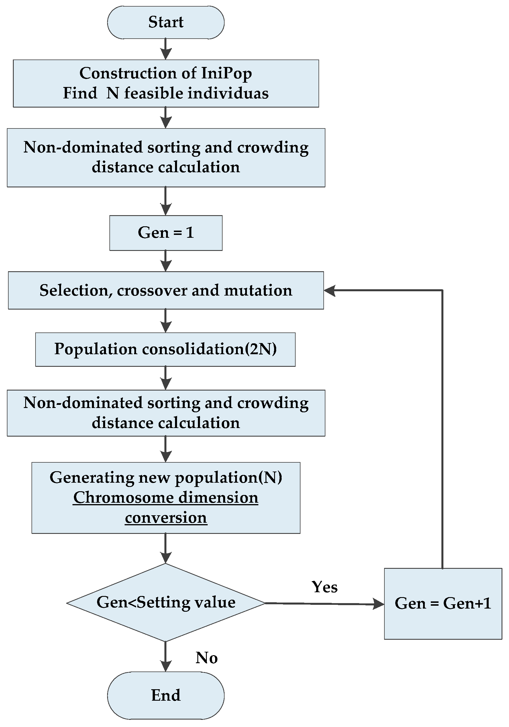
The NSGA-II is based on an elite principle, and it adopts an explicit diversity retention mechanism and emphasizes non-dominated solutions. Initial populations of size N are generated randomly, and then a first-generation offspring population is obtained by the selection, crossover, and mutation of the genetic algorithm after non-dominant sequencing. Second, it is different from the first generation in following generations. It mainly combines the populations of the parent and the offspring, and after they are quickly non-dominated, it calculates the crowding degree of the individual in the non-dominant layer. The appropriate individuals are selected by non-dominant relationships and the results of individual crowding degrees to form a new population. At last, a new subpopulation is created by the basic operation of the genetic algorithm. Then these operations repeat until the conditions for program termination are satisfied. The specific implementation process of the NSGA-II is depicted in Figure 2.

Before we started the formal experiment, we did some preliminary pre-experimental calculations. We found that when the generations of the iteration are too high, for example, 100,000, the NSGA-II usually cannot find a feasible solution because the dimension of the search space is too high. Moreover, for most evaluation functions, the decision variables are one-dimensional, but in our paper, $arrang{e}_{i^{m}k{n}^k}$ is three-dimensional. Therefore, in order to improve the performance of the NSGA-II in finding a Pareto solution, we designed the following improved algorithm. The following is a detailed description of some of the key steps in the proposed algorithm.

3.2.1. Initial Population

In order to improve the quality of the Pareto solution and reduce the optimization time, we improved the initialization phase and defined a new initialization process, mainly by adding constraints to randomly generate the initial population IniPop. More specifically, the constraints in (10–15) are imposed on the initialization function, so that the generated chromosomes are the feasible solutions that satisfy the proposed model constraints, thus forming the initial population of N feasible solutions. The initial population generated affects the convergence of the algorithm: It is also better and more meaningful than the purely randomly generated population of the NSGA-II, and IniPop is also a good seed for the solution of the next generation. On the basis of initialization, the population evolves until the defined number of generations. The pseudo code of the construction process of the initial population IniPop is shown in

Table 5. Construction Algorithm of IniPop.

Algorithm: Construction of IniPop

Data: N

Result: IniPop of N individuals

i: =0;

IniPop = Φ;

While i! = N do

/* imposed the constraints */

/* find the chromosomes randomly */

Find a chromosomei as a feasible solution (or suboptimal) satisfying the constraints;

IniPop = IniPop ∪ chromosomei;

i: = i+1;

end

.

3.2.2. Non-Dominant Sorting and Crowding Distance Calculation

The initial population is sorted using a non-dominated sort. This process returns the sorting value and the crowding distance corresponding to each individual, which is a two-column matrix, and adds sorting values and crowding distances to the chromosome matrix. What is obtained at last is a population matrix that already contains rank and crowding distance and that has been sorted by sorting rank.

3.2.3. Selection, Crossover, and Mutation

The selection process uses a tournament selection approach, which randomly selects two individuals at a time and preferentially selects individuals with a high ranking. If the ranking is the same, it prefers to select individuals with a large crowding distance.

The crossover algorithm selects the simulated binary crossover (SBX). SBX mainly simulates the principle of a single-point crossover based on binary strings and applies it to chromosomes expressed in real numbers. The two parent chromosomes are cross-operated to produce two progeny chromosomes, so that the relevant pattern information of the parent chromosome is protected in the subchromosomes. The mutation uses a general polynomial mutation.

3.2.4. Generating New Populations (Elite Strategy)

The elite strategy keeps the good individuals in the parent directly within the offspring to prevent the obtained Pareto optimal solution from being lost. First, the parent population $C_i$ and the child population $D_i$ are synthesized into a population $R_i$. Then, a new parent population $C_{i+1}$ from the population $R_i$ is generated according to the following rules:

(1) According to the order of Pareto rank from low to high, the whole layer population is put into the parent population $C_{i+1}$ until a layer of the individual cannot be put into the parent population $C_{i+1}$;

(2) The individuals of the layer are sorted according to the crowding distance from large to small and then placed in the parent population $C_{i+1}$ until the parent population $C_{i+1}$ fills up.

3.2.5. Evaluation Function Stage

Generally, a chromosome is one-dimensional, but in our paper, the decision variable $arrang{e}_{i^{s}k{n}^k}$ is three-dimensional. Thus, we proposed a new conversion method after generating a new population (replace chromosome): When a new population is generated, we convert one-dimensional variables into three-dimensional variables using the corresponding rules of the design based on solid geometry properties. The one-dimensional vectors are divided into multidimensional cube vectors of $i^s\ast k\ast n^k$ in order to calculating fitness values.

Meanwhile, after the feasible chromosomes undergo crossover, mutation, and other processes, they may be not feasible. Thus, in order to get a completely feasible solution again, we judge if the obtained chromosomes are feasible in the evaluation function calculation stage. If they meet all the constraints, the evaluation objective values are calculated, and if not, they re-enter initialization.

4. Case Study and Computational Results

In terms of the series of surgical scheduling problems described in Section 2.1, the following cases were used to verify the comparison: (1) Based on the GPA, (2) based on the improved NSGA-II, and (3) based on the actual scheduling of the hospital, thereby verifying the pros and cons of each approach.

In this section, we verify the correctness of the proposed MILPM (1)–(15) and evaluate the effectiveness of the proposed algorithms through two case experiments. First, we used a case to verify the models for Phases 1 and 2 and the proposed GPA solution. Then another case was used to demonstrate the superiority and effectiveness of the improved NSGA-II approach for solving multi-objective models in Phase 2.

The case study involved the SSs of a hospital in Beijing, China. In the public OR department, there were 16 public ORs (one of which was a special OR) that could be allocated to 10 SSs, so 15 ORs were available. The normal opening time of each OR was 8 h per day. However, when a surgery was not completed, overtime work was allowed, and the extra work was paid. The data were collected from October 2018 to November 2018 for a period of one month, with about 1200 elective patients admitted for treatment. The data mainly included the date of admission, the surgery date, the type of illness, the surgery’s start and end time, the attending doctors and nurses, and OR cost, etc.

4.1. Case 1: The Exact Algorithm (GPA)

Generally, each SS could get surgery data 3 days in advance, so the period of allocation was 3 days. In order to match the actual situation, we selected a total of 85 cases of surgeries in the hospital on 15, 16, and 17 October 2018 for discussion in case 1.

4.1.1. Computational Results of Phases 1 and 2

Phase 1. According to the data, for the next 3 days, the available time of 15 ORs in the hospital was 360 h, and the planned surgery time of 10 SSs was 381.32 h, exceeding the 360 h that the ORs could provide. The total minimum demand was 360 h, which was equal to the total OR time of 360 h, which could meet the minimum demand of the SSs, so these data were feasible.

We summarize the raw data for each SS in

Table 6. Raw data for each SS in Phase 1.

Surgical Specialty	Surgery Time		Income per Unit	Overtime Cost	Number of ORs (New)
	Total Time (h)	Minimum Time (h)
Gynecology	36.11	33	978	600	1
Otorhinolaryngology	26.41	22	547	342	1
Hepatobiliary	43.29	38	324	212	1
Orthopedics	27.73	23	923	322	1
Stomatology	30.11	26	567	122	1
Urology	29.01	28	1200	860	1
General surgery	30.78	29	300	120	1
Neurosurgery	56.63	54	250	100	3
Pediatrics	48.26	46	344	200	2
Oncology	52.99	50	134	100	3

: total estimated duration of surgery, income per unit time, overtime cost unit time, and number of ORs allocated to each SS. The estimated duration here mainly includes (1) anesthesia time before the surgery starts, (2) operation time in the OR, and (3) anesthesia recovery time after surgery. The estimated duration depends on the complexity of the procedure and the experience of the medical staff. All models were coded on a 64-bit PC by using ILOG CPLEX 12.8.

Table 7. Computational results for each SS in Phase 1.

Surgical Specialty	Surgery Time		Income per Unit	Overtime Cost	Number of ORs (New)
	Total Time (h)	Minimum Time (h)
Gynecology	36.11	33	978	600	2
Otorhinolaryngology	26.41	22	547	342	1
Hepatobiliary	43.29	38	324	212	2
Orthopedics	27.73	23	923	322	1
Stomatology	30.11	26	567	122	1
Urology	29.01	28	1200	860	1
General surgery	30.78	29	300	120	1
Neurosurgery	56.63	54	250	100	2
Pediatrics	48.26	46	344	200	2
Oncology	52.99	50	134	100	2

reports the computational results.

Phase 2. In our case study, 10 instances were generated corresponding to 10 different SSs based on Phase 1. As in the above, OR time allocation was completed in Phase 1. On this basis, the 10 instances are listed in

Table 8. Problem instances.

Instance	OR	OR Time (h)*3 days	Patient List	Total Surgery Time (h)	Mean Surgery Time (h)
I1	2	16*3	9	36.11	4.01
I2	1	8*3	6	26.41	4.40
I3	2	16*3	9	43.29	4.81
I4	1	8*3	6	27.73	4.62
I5	1	8*3	9	30.11	3.35
I6	1	8*3	5	29.01	5.80
I7	1	8*3	5	30.78	6.16
I8	2	16*3	15	56.63	3.78
I9	2	16*3	8	48.26	6.03
I10	2	16*3	13	52.99	4.08

.

In our models, the solution idea of the cyclic schedule was that it was necessary to select the surgeries from the initial surgery pool L₁ (patient list) and schedule them on the first day. Then the remaining surgeries constituted a new surgical pool L₂. After that, we selected surgeries from L₂ and arranged them on the second day according to the first day’s schedule, and so on, so as to realize the essence of the cyclic schedule. Our scheduling period was 3 days. All surgical cases we considered were elective and the surgical duration was predicted by surgeons, so this schedule would take a three-day cycle.

The solution idea of the GPA was to give the objective priority according to its importance and find the optimal solution of the next priority objective according to the optimal solution of the previous priority objective until the common optimal solution was found. All transformed models were solved by using ILOG CPLEX 12.8. Because the models had four objectives, the final results were gotten after four computations.

Instance 10 was chosen to be presented here. There were 13 surgeries arranged over 3 days in the patient list (Instance 10), as shown in Table 7. First, we selected surgeries from the patient list and arranged them for the first day, then did the same for the second day and the third day. Others besides Instance 10 were done in the same way. The original schedule and the results for Instance 10 are presented in

Table 9. The original schedule of Instance 10.

Day in Period	OR	Surgery Serial Number	Duration of Surgery (h)	Total Surgery Time (h)
1	1	1	3.57	8.33
		2	1.75
		3	1.00
		4	2.01
	2	5	4.58	4.58
	3	6	9.87	9.87
2	1	7	4.74	8.32
		8	1.25
		9	2.33
	2	10	4.33	4.33
	3	11	8.00	8.00
3	1	12	3.89	9.56
		13	5.67
	2 and 3	unscheduled	-	-

and

Table 10. The results of Instance 10.

Day in Period	OR	Surgery Serial Number	Duration of Surgery (h)	Total Surgery Time (h)
1	1	10	4.33	8.22
		12	3.89
	2	1	3.57	9.16
		8	1.25
		4	2.01
		9	2.33
2	1	5	4.58	9.32
		7	4.74
	2	6	9.87	9.87
3	1	11	8.00	8.00
	2	13	5.67	8.42
		3	1.00
		2	1.75

.

4.1.2. Comparison and Discussion of GPA Solutions with Real Schedules

As for OR allocation results among SSs, which are presented in Table 7, the total number of ORs was equal, but other indexes changed. It can be seen from Figure 3 that the idle ratio and the overtime ratio decreased, while net income increased, which proved that OR efficiency increased in the new allocation scheme.

According to the results in Table 10 about Instance 10, 6 surgeries were arranged on the first day, 3 surgeries on the second day, and 4 surgeries on the third day. The specific scheduling results are shown in the Gantt chart in Figure 4 and are compared to the original hospital schedule plan in Figure 5. The red blocks represent the first day, the blue represent the second day, and the green represent the third day.

In the above, we can see that the total number of scheduled surgeries was the same, but OR utilization and equilibrium varied too much. For the second objective in the models, the overtime and idle time are the differences between the total time for each OR over the three days and the normal opening time (8 h). As shown in

Table 11. Comparison of various indicators (overtime and idle time).

	OR	1	2	3
Day 1	Original	0.33	−3.42	1.87
	New	0.22	1.16	-
Day 2	Original	0.32	−3.67	-
	New	1.32	1.87	0.00
Day 3	Original	1.56	−8.00	−8.00
	New	0.00	0.42	-

, when comparing the total OR time to the standard time, it can be seen that the original schedule had a long overtime and idle time. The total idle time was 23.34 h, and the OR utilization rate was 67.58%. There was no idle time after optimization, the overtime was relatively small, and it was relatively balanced. Simultaneously, the OR utilization rate was 89.61%, which achieved a basic optimization goal, improved the OR utilization rate, and increased hospital income.

For the third objective (minimizing the working time equalization rates among ORs), we first conducted a qualitative analysis. Figure 6, Figure 7 and Figure 8 are plotted for comparison according to the total time of each OR in the three days before and after the optimization. As shown in the figures, the curve of the original schedule changed greatly, and the utilization rate of each OR was different. Besides, there was a load difference in each OR, and this difference was embodied in the fact that some of the ORs had too many patients, resulting in a crowded situation, while the others were relatively idle. This service efficiency was uneven, which inevitably resulted in low overall service efficiency and unimproved patient satisfaction. The reason for the imbalance in the utilization rate of the ORs was that the SSs had adopted the principle of FCFS, and there was no comprehensive scheduling of the ORs according to the specific situation.

After optimization, the whole curve was relatively smooth. It seems that the utilization rate among the ORs was approximately the same, the completion time between the ORs was balanced, and the equalization rate was significantly improved. Besides a qualitative analysis by line chart, SPSS 19.0 was used to describe the statistical characteristics of the OR time before and after the optimization for a quantitative analysis.

According to the results of the descriptive statistics in

Table 12. Variance analysis of total OR time.

State	N	Minimum Value	Maximum Value	Mean Value	Variance
Original	3	0.00	9.87	5.89	13.24
New	2	8.00	9.87	8.83	0.44

, the standard deviation was 0.44 after optimization, which was significantly smaller than the pre-optimization of 13.24. It can be concluded that the equilibrium rate between ORs significantly improved, and the mean OR time was closer to that of the real ORs. All of these results proved the effectiveness of the proposed models and the GPA.

As described in the introduction in Section 1, besides the three objectives considered in this paper, patient waiting time is also a key indicator considered in the OR scheduling research field today. However, patient waiting time in the optimized scheme obtained in Instance 10 seems to have been more than before. This was because we considered OR cost and other factors in Phase 1, and the number of assigned ORs to an SS was reduced from the previous 3 to 2. Then, in Phase 2, although the number of surgeries scheduled, the overtime and idle time in the ORs, and the OR balance rate for the optimized scheme were similarly better than those of the original scheme, patient waiting time was not satisfactory. In order to verify the optimization of patient waiting time in our optimized scheme, we assumed that Instance 10 was assigned 3 ORs in Phase 1, and then we recalculated the models through the GPA proposed in Phase 2. The resulting Gantt chart is shown in Figure 9.

From Figure 9, we found that when patient waiting time was the measured standard and OR cost was not particularly important, we could open three ORs. As a result, all of the surgeries in the SS could be completed within 2 days in our solution, significantly reducing patient waiting time and increasing patient satisfaction.

4.2. Case 2: The Heuristic Algorithm (Improved NSGA-II)

In Section 4.1, some small-sized cases were discussed in detail. Especially in Phase 2, there was a multi-objective model, and while using the GPA and CPLEX is sometimes subjective, this approach may not solve the large-sized cases. In response to these shortcomings, we conducted another experiment to verify the application of the improved NSGA-II approach. Based on the situation, the real data generated realistic random instances to study more complex SSs and ORs, and the constructed instances were allocated ORs (so Phase 1 could be omitted). To investigate the interaction between objective functions and how management strategies affected patient lists and OR efficiency, we conducted different experiments. Meanwhile, the computational results with two approaches are presented below and discussed.

4.2.1. Data Description, Experiment Design, and Model Coding

In our computational experiments, by using the real surgical data obtained from a top three hospital in Beijing, we randomly generated the number of ORs allocated to each SS in Phase 1 according to the nth power of 2 and selected the actual surgical information of 10, 100, or 1000 patients to form the test cases. Then, 9 different sets of benchmark instances were generated. This was done by considering three different SS sizes (2, 8, and 16 ORs) and three different waiting lists according to 10, 100, or 1000 surgical cases for each SS. In more detail, we refer to these sets as (a, b, c), where a is the SS size, b is the waiting list, and c is the SS (i.e., (2, 10, 1) refers to an instance with 2 ORs and 10 surgical cases on the waiting list of an SS). The nine instances were (2, 10, 1), (8, 10, 1), (16, 10, 1), (2, 100, 1), (8, 100, 1), (16, 100, 1), (2, 1000, 1), (8, 1000, 1). and (16, 1000, 1).

The scheduling of each procedure was encoded with a binary chromosome. After the three-dimensional chromosomes were tiled into one-dimensional chromosomes, in each OR, the position of each chromosome represented the surgical sequence in which the surgery was arranged in the OR (example shown in Figure 10).

Table 13. Parameter settings.

Parameter Values of the Improved NSGA-II
pop = 200
gen = 5000
Tour = 2
mu = 20
mum = 20
crossover rate = 0.9
mutation rate = 1/k

lists some of the parameter values we used in the calculation of the experiment, where the mutation rate = 1/k, where k is the length of the string of the relevant instance. At the same time, MILPM (7–15) was coded in MATLAB R2016a. When the program ran the set generation, the program terminated.

4.2.2. Experiment Results and Analysis

As for our cases, the problem we solved was based on the description in Section 2.1. In this section, mainly in order to verify the effectiveness of the improved NSGA-II approach for solving large-scale multi-objective problems, the problem we consider is mainly about Phase 2 scheduling in a single SS in a scheduling period. First we selected surgeries from the patient waiting list, and then we arranged the specific ORs and times for them. In this section, the idea that we are ignoring Phase 1 is also reflected in the process of generating test cases in Section 4.2.1. The experimental framework proposed in this paper was based on the complexity and characteristics of the proposed correlation models and nine scene instances based on actual background features. The specific instance descriptions are presented in

Table 14. Experiment design: identifier of the experiment.

Instance (SS Size, Waiting Lists, One SS)	Number of Constraints	Length of Chromosomes (m)	Max Surgery Time (h)	Min Surgery Time (h)	Mean Surgery Time (h)
(2, 10, 1)	40	200	8.35	1.92	4.02
(8, 10, 1)	100	800	6.75	2.12	4.41
(16, 10, 1)	180	1,600	10.58	2.45	4.81
(2, 100, 1)	400	40,000	14.33	1.80	4.62
(8, 100, 1)	1,000	80,000	7.83	1.74	3.35
(16, 100, 1)	1,800	160,000	9.27	4.59	5.82
(2, 1000, 1)	4,000	4,000,000	9.25	3.50	6.16
(8, 1000, 1)	10,000	8,000,000	7.23	0.41	3.78
(16, 1000, 1)	18,000	16,000,000	11.33	1.24	6.03

.

Maximizing the number of scheduled patients in all ORs in a certain SS, minimizing underutilization and overall overtime cost in the ORs, and aiming to balance between the ORs according to the standard deviation of the OR working time were the optimization bases. Considering the basic condition of the patient waiting list in each SS, each scheduling schedule defined four aspects: (1) the number of ORs (i.e., OR time) allocated for each SS (already solved in Phase 1), (2) the surgeries selected from the surgery pool, (3) appointed ORs for the selected surgeries, and (4) the surgical sequence in each OR.

Our computational experiments were performed on MATLAB R2016a with a 2.8 GHz 64-bit PC by running the NSGA-II. After computation with sufficient generations, a set of Pareto solutions could be obtained, called the Pareto front, which was a trade-off between the three objectives and could represent a set of OR scheduling schemes. In general, since different scheduling schemes may have had the same objective function value, the number of solutions obtained was smaller than the actual population N. In order to prove the validity of the proposed method, we selected the first 10 solutions of the output in the example (16, 100, 1) and show the details in

Table 15. First 10 non-dominated Pareto solutions for (16, 100, 1).

Objective Function	Schedules										Min	Max
	1	2	3	4	5	6	7	8	9	10
(max) Objective 1	22	35	16	16	25	34	37	37	33	39	16	39
(min) Objective 2	7.67	22.43	6.04	5.34	14.54	19.93	21.13	23.43	20.06	31.56	5.34	31.56
(min) Objective 3	0.296	1.161	0.474	0.238	2.471	2.523	2.519	2.633	2.419	2.903	0.238	2.903

.

Actually, we could get a set of Pareto solutions in this case. For this paper, we selected the first 10 feasible solutions in order from the output results for a concrete display. For a set of feasible solutions, they had three conflicting objectives: the number of scheduled surgeries, the overtime in the ORs, and the idle time in the ORs. In the decision-making process, this is mainly based on the preferences of hospital managers to make balanced choices among these three objectives. If the manager wants to arrange as many surgeries as possible to improve patient satisfaction, then he/she can select the one with a maximum value of Objective 1: The maximum number of scheduled surgeries is the priority measure, and the solution with a maximum value of Objective 1 is selected as the optimal solution. On the other hand, if the hospital measures the surgical cost of the ORs and the satisfaction of the medical staff, the minimum value of Objective 2 is the considered solution when selecting the optimal solution. If the surgical time in each OR should be consistent in the surgical department, the hospital managers should select the solution with the minimum value of Objective 3 as the optimal solution.

By observing Table 15, we can see that for OR scheduling scheme 10, the number of scheduled surgeries was the largest. If only the patient’s satisfaction was considered, scheme 10 could be chosen as the best solution, but this was at the expense of increasing the overtime and free time in the ORs. Besides, the OR imbalance rate also reached a maximum. On the other hand, for scheme 4, the optimal value of Objective 2 was achieved, but Objective 1 was the worst value here. At the same time, there was a similar phenomenon between Objective 3 and Objective 1. However, it was gratifying that OR utilization seemed to be more balanced when there was less overtime and idle time in the ORs, but there were some anomalies, as in scheme 1.

Table 16. Computational results: minimum and maximum values of the three objective functions and CPU time (in min).

Instance (SS Size, Waiting Lists, One SS)	(Max) Objective 1		(Min) Objective 2		(Min) Objective 3		CPU Time/Min
	Min	Max	Min	Max	Min	Max
(2, 10, 1)	8	10	3.88	5.78	0.083	1.472	6
(8, 10, 1)	8	10	98.50	113.01	0.079	0.991	7
(16, 10, 1)	9	10	267.30	301.69	0.071	1.688	11
(2, 100, 1)	13	16	2.07	12.41	0.112	4.654	21
(8, 100, 1)	50	56	10.05	30.08	0.097	1.066	32
(16, 100, 1)	33	39	5.34	23.55	0.238	2.903	50
(2, 1000, 1)	14	15	13.55	24.368	0.076	5.966	98
(8, 1000, 1)	57	62	3.18	10.12	0.107	3.994	150
(16, 1000, 1)	98	102	4.72	34.51	0.067	1.554	230

summarizes the maximum and minimum values of each objective function and their calculation times in nine instances. As we found and expected, the optimization of one objective was always accompanied by the loss of other objectives: This is the meaning of Pareto optimization.

The above methods we propose could be used to generate a Pareto solution that could be used to balance the multiple criteria we considered: maximizing the scheduled surgery time, minimizing overtime and idleness in the ORs, and increasing the balance rate of the ORs, etc. The basic principle of a Pareto solution is that there is no guarantee that the objective value will be optimized without worsening other criteria. A histogram can be intuitive in helping decision-makers understand content. Figure 11 and Figure 12 show the first five non-dominated solutions of (8, 100, 1), which were characterized by 8 ORs and 100 surgeries in an SS. Figure 11 shows the respective objective function values for the five scheduling schemes, and Figure 12 shows a comparison of each objective function value in each scheme.

4.2.3. Comparison and Discussion

To complete and show the main differences in all of the objectives, we now discuss the performance of the proposed GPA and improved NSGA-II approaches in the benchmark instances. The idea of the GPA was to show the main differences with a single objective: We solved the transformed models by maximizing objective function 1, minimizing objective function 2, and minimizing objective function 3 based on benchmark instances by running ILOG CPLEX 12.8. In order to verify the validity of the proposed improved NSGA-II, we chose the best values of Objective 1, Objective 2, and Objective 3 from Pareto solutions to compare to those of the exact solutions in the GPA. The found feasible solutions are reported in

Table 17. Comparison between the GPA and the improved NSGA-II approach.

Instance (SS Size, Waiting Lists, One SS)	GPA				Improved NSGA-II
	Objective 1	Objective 2	Objective 3	CPU Time	(Max) Objective 1	(Min) Objective 2	(Min) Objective 3	CPU Time
(2, 10, 1)	10	7.56	2.764	0.566	10	3.88	0.083	6
(8, 10, 1)	10	132.70	1.063	0.578	10	98.50	0.079	7
(16, 10, 1)	10	312.40	1.759	0.822	10	267.30	0.071	11
(2, 100, 1)	12	3.93	2.663	2	16	2.07	0.112	21
(8, 100, 1)	45	12.10	2.731	9	56	10.05	0.097	32
(16, 100, 1)	89	8.71	4.564	12	39	5.34	0.161	50
(2, 1000, 1)	-	-	-	Unsolved	15	13.55	0.076	98
(8, 1000, 1)	-	-	-	Unsolved	62	3.18	0.107	150
(16, 1000, 1)	-	-	-	Unsolved	102	4.72	0.067	230

, where each row of the table reports the three objective values over nine realizations belonging to the benchmark set. The first column in the table shows the name of the benchmark set (a, b, c). Columns 2–5 report the performance indexes of the GPA, while in the next columns (6–9) we report the same performance indexes for the improved NSGA-II approach. More specifically, columns 2, 3, and 4 show the values of each objective value. Column 5 reports the CPU time required by the GPA where the gap is zero. Columns 6, 7, and 8 show the best values of the three objective functions of the solutions found by the improved NSGA-II approach. Finally, column 9 indicates the CPU time required to compute the heuristic solution: the improved NSGA-II.

As for the first objective function, the values between the two approaches were the same (10, 10, and 10) when there were small-sized instances (e.g., (2, 10, 1), (8, 10, 1), and (16, 10, 1)), because when the patient list was 10, there were enough ORs to serve patients correspondingly. When the instance size increased, the scheduled patients (with the improved NSGA-II) were 16, 56, 39, 15, 62, and 102, which were bigger values than those with the GPA. Moreover, when the instance size increased to a certain scale, the models could not be solved by the GPA. On the other hand, the OR overtimes and idle times of the second objective function solved by the GPA were 7.56, 132.70, 312.40, 3.93, 12.10, and 8.71, which was worse than with the proposed improved NSGA-II approach. The same was true for the third objective function. In addition, the GPA used less CPU time than the proposed approach did for small-sized instances (e.g., (2, 10, 1), (8, 10, 1), etc.). This exceeded the computing power of the GPA when the large-scale instances were created (e.g., (2, 1000, 1), (8, 1000, 1), etc.), but the proposed improved NSGA-II approach showed good computing performance for the models.

We also describe the several indexes specifically in Figure 13. The first, Figure 13a, describes the first objective function values between the two approaches. The second, Figure 13b, describes the second objective function, and Figure 13c describes the third one. The last describes the CPU time. For the GPA, the objective values that could not be calculated were uniformly set to 0, indicating that they did not exist. Obviously, the approaches that we propose had better results in all of the objectives and high computational efficiency in solving large-scale problems.

Besides the better performance of the values of all objective functions and CPU time, the advantages of our proposed improved NSGA-II approach were mainly reflected in the decision solution sets. For Pareto collections with more non-dominated solutions, the decision support scheme (DSS) in this paper helps decision-makers make better choices from multiple solutions. For example, non-dominant solutions can perform an integrated analysis based on different objective values, thereby increasing the visual analysis of different solutions, as shown in Figure 11 and Figure 12. Hospital managers can choose the appropriate schedule easily on the basis of the situation and the requirements. How the OR is allocated, how SS requests are met, and which patient graphical representations are arranged help in studying how the schedules differ between them. A more complex DSS can analyze OR overtime, free time, and underutilized changes by selecting different schedules. Other more complex DSS functions can be defined and implemented to make decisions easier.

5. Conclusions

The key to effectively solving OR scheduling problems is to balance surgical needs and available OR resources in an economical and effective way. To this end, we proposed a multiphase OR scheduling approach that addresses two different decision levels, allowing for updates to the waiting list status, availability of the ORs, and staff hours during the next planning period.

The designed OR resource allocation model and the integrated multi-objective cyclic OR scheduling model produce a set of optimal decisions that link conflicting objectives within the SSs with hospital managers and patients. On the basis of completion of OR time allocation, the number of surgical arrangements is maximized, and overtime and idle time in the ORs are reduced to increase utilization of the ORs. In fact, we solved the problems of OR time allocation, the master surgery schedule, and other issues in an integrated and independent way.

In the process of solving the models, we put forward the GPA combined with the AHP to accurately solve the MSS model and compared the solution results to the actual OR schedule of a hospital, verifying the effectiveness of the models and the solution approach. In addition, due to the convergence shortcomings of the NSGA-II, we proposed an improved genetic algorithm to overcome this problem effectively in the solution. The improved algorithm defines a new initialization process to construct a new initial population with a suitable set of feasible chromosomes that meet the constraints that are the seeds of evolutionary computation. In the evaluation phase, we determined whether the chromosomes with a cross-mutation met the constraints. At the same time, conformance constraints were retained, and nonconformance constraints were reinitialized and supplemented. The resulting set of possible Pareto solutions could balance conflicting objectives while ensuring that the criteria could not be improved without destroying other criteria. Different solutions have different qualities and costs of service, and the overall evaluation of different solutions allows managers to make better choices.

In our paper, there were some assumptions about the uncertainty of the ORs and surgeries (such as uncertainties about surgical duration, the patients arriving, and the ORs’ other resources) in order to further develop a more effective OR scheduling model system. The optimization method and algorithm developed in this paper can consider other resources (e.g., the availability of beds, recovery beds, medical staff, and other factors) and different optimization objectives in evaluating the performance of a scheme.

In addition, dynamic uncertainty is an important point that we should consider. The surgical time of a hospital has great uncertainty. The duration of a surgery is affected by many factors, such as the skill level of the doctor, the degree of fatigue, and the physical state of the patient. Meanwhile, due to the frequent occurrence of emergency surgery, the OR schedule is unstable. Thus, our next step is to pay attention to these issues.

In addition, we will also conduct an in-depth study of the NSGA-III, applying it to an OR schedule to improve the accuracy of the solutions.

References

1. Bharathwaj, V.; Pratik, J.P.; Rosalyn, S.; April, B.; Jennie, G. A dual bin-packing approach to scheduling surgical cases at a publicly-funded hospital. Eur. J. Oper. Res. 2013, 224, 583–591. [Google Scholar]
2. Cao, X.T.; Dong, J.; Song, F. Discussion of Statistical Indexes and Methods Reflecting the Using Efficiency of Operating Room. Chin. J. Heal. Static. 2003, 20, 82–83. [Google Scholar]
3. Sieber, T.J.; Leibundgut, D.L. Operating room management and strategies in Switzerland: results of a survey. Eur. J. Anaesthesiol. 2002, 19, 415–423. [Google Scholar] [CrossRef]
4. Cardoen, B.; Demeulemeester, E.; Beliën, J. Operating room planning and scheduling: A literature review. Eur. J. Oper. Res. 2010, 201, 921–932. [Google Scholar] [CrossRef]
5. Lamiri, M.; Xie, X.; Dolgui, A.; Grimaud, F. A stochastic model for operating room planning with elective and emergency demand for surgery. Eur. J. Oper. Res. 2008, 185, 1026–1037. [Google Scholar] [CrossRef]
6. Ozcan, Y.A. Quantitative Methods in Health Care Management. J. Oper. Res. Soc. 2009, 58, 1119–1120. [Google Scholar]
7. Magerlein, J.M.; Martin, J.B. Surgical demand scheduling: A review. Health Serv. Res. 1978, 13, 418–433. [Google Scholar]
8. Blake, J.T.; Carter, M.W. A goal programming approach to strategic resource allocation in acute care hospitals. Eur. J. Oper. Res. 2002, 140, 541–561. [Google Scholar] [CrossRef]
9. Dexter, F.; Ledolter, J.; Wachtel, R.E. Tactical decision making for selective expansion of operating room resources incorporating financial criteria and uncertainty in subspecialties’ future workloads. Anesth. Analg. 2005, 100, 1425–1432. [Google Scholar] [CrossRef] [PubMed]
10. Guinet, A.; Chaabane, S. Operating theatre planning. Int. J. Prod. Econ. 2003, 85, 69–81. [Google Scholar] [CrossRef]
11. Ozkarahan, I. Allocation of surgeries to operating rooms using goal programming. J. Med. Syst. 2000, 24, 339–378. [Google Scholar] [CrossRef]
12. Testi, A.; Tanfani, E.; Torre, G.A. Three-phase approach for operating theatre schedules. Health Care Manag. Sci. 2007, 10, 163–172. [Google Scholar] [CrossRef] [PubMed]
13. Ogulata, S.; Erol, R.A. Hierarchical multiple criteria mathematical programming approach for scheduling general surgery operations in large hospitals. J. Med. Syst. 2003, 27, 259–270. [Google Scholar] [CrossRef] [PubMed]
14. Cardoen, B.; Demeulemeester, E.; Beliën, J. Optimizing a multiple objective surgical case sequencing problem. Int. J. Prod. Econ. 2009, 119, 354–366. [Google Scholar] [CrossRef]
15. Beliën, J.; Demeulemeester, E.; Cardoen, B. A decision support system for cyclic master surgery scheduling with multiple objectives. J. Sched. 2009, 12, 147–161. [Google Scholar] [CrossRef]
16. Marler, R.T.; Arora, J.S. The weighted sum method for multi-objective optimization: new insights. Struct Multidisc. Optim. 2010, 41, 853–862. [Google Scholar] [CrossRef]
17. Meskens, N.; Duvivier, D.; Hanset, A. Multi-objective operating room scheduling considering desiderata of the surgical team. Dec. Support. Syst. 2013, 55, 650–659. [Google Scholar] [CrossRef]
18. Zhao, Z.; Li, X. Scheduling elective surgeries with sequence-dependent setup times to multiple operating rooms using constraint programming. Oper. Res. Health Care 2014, 3, 160–167. [Google Scholar] [CrossRef]
19. Bosch, P.M.; Dietz, D.C. Minimizing expected waiting in a medical appointment system. IIE Trans. 2000, 32, 841–848. [Google Scholar] [CrossRef]
20. Raphael, E.C.; Finardi, E.C.; Silva, E.L.; Santos, M.L. Comparing stochastic optimization methods to solve the medium-term operation planning problem. Comput. Appl. Math. 2011, 30, 289–313. [Google Scholar]
21. Guerriero, F.; Guido, R. Operational research in the management of the operating theatre: a survey. Health Care Manag. Sci. 2011, 14, 89–114. [Google Scholar]
22. Gupta, D. Surgical suites’ operations management. Prod. Oper. Manag. 2010, 16, 689–700. [Google Scholar] [CrossRef]
23. Sandberg, W.S.; Daily, B.; Egan, M.; Stahl, J.E.; Goldman, J.; Wiklund, R. Deliberate perioperative systems design improves operating room throughput. Anesthesiology 2005, 103, 406–408. [Google Scholar] [CrossRef]
24. Lamiri, M.; Frédéric, G.; Xie, X. Optimization methods for a stochastic surgery planning problem. Int. J. Prod. Econ. 2009, 120, 400–410. [Google Scholar] [CrossRef]
25. Pulido, R.; Aguirre, A.M.; Ortegamier, M.; Álvaro, G.; Carlos, A.M. Managing daily surgery schedules in a teaching hospital: a mixed-integer optimization approach. BMC Health Serv. Res. 2014, 14, 1472–1485. [Google Scholar] [CrossRef]
26. McIntosh, C.; Dexter, F.; Epstein, R.H. The impact of service-specific staffing, case scheduling, turnovers, and first-case starts on anesthesia group and operating room productivity: a tutorial using data from an Australian hospital. Anesth. Analg. 2006, 103, 1499–1516. [Google Scholar] [CrossRef]
27. Kuo, P.C.; Schroeder, R.A.; Mahaffey, S.; Bollinger, R.R. Optimization of operating room allocation using linear programming techniques. J. Am. Coll. Surg. 2003, 197, 889–895. [Google Scholar] [CrossRef]
28. Jebali, A.; Hadjalouane, A.; Ladet, P. Operating rooms scheduling. Int. J. Prod. Econ. 2006, 99, 52–62. [Google Scholar] [CrossRef]
29. Wang, S.; Roshanaei, V.; Aleman, D.M.; Urbach, D.R. A discrete event simulation evaluation of distributed operating room scheduling. IIE Trans. Health. Syst. Eng. 2016, 6, 236–245. [Google Scholar] [CrossRef]
30. Guo, M.; Wu, S.; Li, B.; Song, J.; Rong, Y. Integrated scheduling of elective surgeries and surgical nurses for operating room suites. Flex Serv. Manuf. J. 2016, 28, 166–181. [Google Scholar] [CrossRef]
31. Guillermo, D.; Rey, P.A.; Wolff, P. Solving the operating room scheduling problem with prioritized lists of patients. ANN Oper. Res. 2016, 258, 395–414. [Google Scholar]
32. Gupta, D.; Natarajan, M.K.; Gafni, A.; Wang, L.; Shilton, D.; Holder, D.; Yusuf, S. Capacity planning for cardiac catheterization: a case study. Health Pol. 2007, 82, 1–11. [Google Scholar] [CrossRef]
33. Hans, E.; Wullink, G.; Vanhoudenhoven, M.; Kazemier, G. Robust surgery loading. Eur. J. Oper. Res. 2008, 185, 1038–1050. [Google Scholar] [CrossRef]
34. Guido, R.; Conforti, D. A hybrid genetic approach for solving an integrated multi-objective operating room planning and scheduling problem. Comput. Oper. Res. 2017, 87, 270–282. [Google Scholar] [CrossRef]
35. Chen, S.Z.; Zhang, X.; Peng, L.G.; Zhang, D.H.; Sun, J.; Liu, Y.Z. Multi-objective optimization of rolling schedule based on cost function for tandem cold mill. J. Cent. South. Univ. 2014, 21, 1733–1740. [Google Scholar] [CrossRef]
36. Cardoen, B.; Demeulemeester, E.; Beliën, J. Operating room planning and scheduling problems: a classification scheme. Int. J. Health Manag. Inform. 2010, 13, 71–83. [Google Scholar]
37. Marques, C.; Eugénia, M. Bicriteria elective surgery scheduling using an evolutionary algorithm. Oper. Res. Health Care 2015, 7, 14–26. [Google Scholar] [CrossRef]
38. Kalyanmoy, D.; Amrit, P.; Sameer, A.; Meyarivan, T. A Fast Elitist Multi-Objective Genetic Algorithm: NSGA-II. IIE Trans. Evol. Comput. 2002, 6, 182–197. [Google Scholar]
39. Srinivas, N.; Kalyanmoy, D. Multi-objective Optimization Using Nondominated Sorting in Genetic Algorithms. Evol. Comput. 1994, 2, 221–248. [Google Scholar] [CrossRef]
Figure 1. Hierarchical structure diagram in Phase 2.
Symmetry 11 00599 g001
Figure 2. Non-dominated Sorting Genetic Algorithm II (NSGA-II) solution approach.
Symmetry 11 00599 g002
Figure 3. Some indexes before and after optimization.
Symmetry 11 00599 g003
Figure 4. Scheduling Gantt chart in Instance 10 via Goal Programming Approach (GPA) (2 allocated ORs).
Symmetry 11 00599 g004
Figure 5. Scheduling Gantt chart in Instance 10.
Symmetry 11 00599 g005
Figure 6. Comparison of the total time in each OR before and after scheduling (Day 1).
Symmetry 11 00599 g006
Figure 7. Comparison of the total time in each OR before and after optimization (Day 2).
Symmetry 11 00599 g007
Figure 8. Comparison of the total time in each OR before and after optimization (Day 3).
Symmetry 11 00599 g008
Figure 9. Scheduling Gantt chart in Instance 10 via GPA (3 allocated ORs).
Symmetry 11 00599 g009
Figure 10. Presentation of a surgical schedule encoded with a binary chromosome.
Symmetry 11 00599 g010
Figure 11. A synoptic representation of the five non-dominated solutions of (8, 100, 1).
Symmetry 11 00599 g011
Figure 12. Comparison of the three objective values of the five non-dominated solutions of (8, 100, 1).
Symmetry 11 00599 g012
Figure 13. Several indexes in different instance sizes between two approaches.
Symmetry 11 00599 g013aSymmetry 11 00599 g013b