The Symmetry in the Noise-Perturbed Mandelbrot Set

Abstract

This paper investigates the destruction of the symmetrical structure of the noise-perturbed Mandelbrot set (M-set). By applying the “symmetry criterion” method, we quantitatively compare the damages to the symmetry of the noise-perturbed Mandelbrot set resulting from additive and multiplicative noises. Because of the uneven distribution between the core positions and the edge positions of the noise-perturbed Mandelbrot set, the comparison results reveal a paradox between the visual sense and quantified result. Thus, we propose a new “visual symmetry criterion” method that is more suitable for the measurement of visual asymmetry.

1. Introduction

In the early 20^th Century, French mathematician Gaston Julia [1] focused on the following simple map:

$$f:\left\{\begin{array}{c}{x}_{n+1}=x_n^2-y_n^2+c_1\hfill \\ y_{n+1}=2x_n{y}_n+c_2,\hfill \end{array}\right.$$

(1)

where $x_n,y_n,c_1,c_2\in \mathbb{R}$. He put forward that such a simple procedure could generate a complicated fractal set, which was named the Julia set.

To analyze the connectivity property of the Julia set with different parameters $(c_1,c_2)$, Mandelbrot [2] revealed another set of classical fractals, the Mandelbrot set (M-set), that was formed with all the values $(c_1,c_2)$ that make its corresponding Julia set connected.

Currently, as one of the most basic sets of fractals and one of the hottest topics of nonlinear science theory, the Mandelbrot set has drawn increasing attention for its theoretical investigations, such as the topological structure analysis [3,4,5], properties [6,7], control [8,9], and high-dimensional developments of such sets [9,10,11]. These theoretical research efforts have resulted in successful applications in interdisciplinary fields, including physics [12], biology [13,14], image encryption [15], and so forth.

Symmetry is always investigated as a geometric property or algebraic structure in nonlinear science. For instance, the property analysis and control of symmetric and asymmetric chaotic systems can be found in [16,17,18]. Early studies on fractals analyzed the symmetry property of the planar M-set generated from map (1) [2] and some generalized maps [19]. Recently, scholars have focused their attention on the symmetry property of the spatial M-set [11,20]. In [20], the authors proved the symmetry of the 3D slice of the M-set generated by an alternative map.

It is noted that stochastic systems are widely applied because they can effectively describe several natural processes. Although the theoretical framework of stochastic fractal systems has not been systematically studied, the graphical exploration of noise-perturbed fractals sets, initiated in [21,22,23] with the aid of computer drawing tools, has attracted significant interest in recent years [24,25,26,27,28,29,30]. Wang et al. studied the structural characteristics of additive noise-perturbed Julia sets [24], called “Julia deviation distance”, and its corresponding graphical tool “Julia deviation plot” was proposed to quantify and visualize noise-perturbed fractal sets in [28,29]. The “Julia deviation distance” method provided an effective algorithm for calculating the total number of points in the noise-perturbed fractals sets. In [30], the authors extended the “Julia deviation plot” [28] into the spatial case by investigating the Julia sets of a complex Lorenz system. Besides, the authors also [30] proposed a “symmetry criterion” method to quantify the effect of noise on the symmetry changes in the spatial Julia set.

Inspired by the research above, the objective of this work is to apply and modify the “Symmetry Criterion” method ($SC$) [30] in a detailed symmetry analysis of the noise-perturbed M-set. Specifically, the contributions of this work are as follows:

(1)

Application of the “symmetry criterion” method [30] to investigate the Mandelbrot set. To the best of our knowledge, the work in [30] was the first study that addressed the quantization of the symmetry destruction of the noise-perturbed Julia set. In this work, we applied it to the research of another fractal set, namely the Mandelbrot set.

(2)

The proposition of a new “visual symmetry criterion” method. It is noted that the current $SC$ method’s principle of calculating the quantized ratio of the symmetric region to the whole M-set is not very effective for measuring some visually-asymmetric sets. Thus, by adding a weight to the “symmetry index”, we modified the $SC$ method to a novel one named the “visual symmetry criterion” method, which is more in line with visual habits.

The remainder of the paper is outlined as follows. Section 2 recalls the definition of the Mandelbrot set and presents the general form of noise-perturbed map (1). In Section 3, the “symmetry criterion” method and its modified version, the “visual symmetry criterion” method are both applied to quantify the symmetry change in the noise-perturbed M-set. Some simulation results are also included. A comparison between the two methods is given in Section 4. In Section 4, we discuss the novelties and limitations of our work. Section 5 concludes this work by pointing out some potential applications of this study.

2. Preliminaries

In this section, the definition of the Mandelbrot set and the general form of noise-perturbed maps are presented.

Definition 1

([2]). The Mandelbrot set of System (1), denoted as $M\left(f\right)$, is the set of all values of parameters $(c_1,c_2)$ under the conditions of $(x_0,y_0)=(0,0)$ such that:

$$\underset{n\to \infty }{lim}|f^n(x_0,y_0,c_1,c_2)|\nrightarrow \infty ,$$

(2)

where $f^n(·)$ represents the n^th iteration of the initial point $(x_0,y_0)$.

Based on the software MATLAB 2014a, the escape-time algorithm [2] that numerically calculates $M\left(f\right)$ is briefly discussed: The lattice $L:[-2,2]\times [-2,2]$ is constructed as the space of initial points $(c_1,c_2)$, i.e., $-2\le c_1\le 2$, $-2\le c_2\le 2$. Then, the initial two intervals are divided into $P\times P(P=4000)$ smaller lattices. As a result, the $P^2$ points in the lattice L are obtained with the following coordinates:

$${\theta }_0=\left\{\begin{array}{c}{c}_1=-2+(i-1)\left(\frac{4}{P-1}\right),\hfill \\ c_2=-2+(j-1)\left(\frac{4}{P-1}\right).\hfill \end{array}\right.$$

Setting $N=500$ as the escape time limit and $R=10$ as the escape radius (the same parameter selection used in [28,29]), the value of the distance r of the $N^{\mathrm{th}}$ iteration of $(x_0,y_0,c_1,c_2)$ from the original point is calculated. Then, all the original points $c_1,c_2$ with $r<R$ form the classical Mandelbrot set $M\left(f\right)$ (see Figure 1).

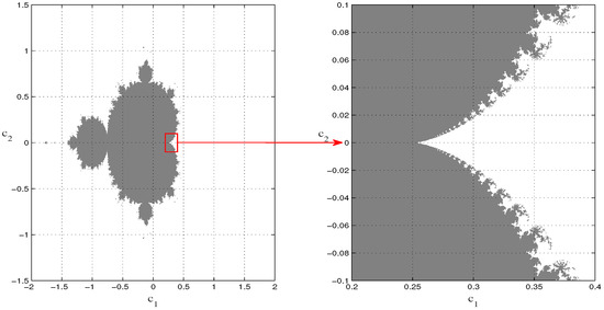
Figure 1. The Mandelbrot set $M\left(f\right)$ of the map (1) without noise.

The additive noise in the map (1), denoted by $f^a$, is defined as:

$$f^a=\left\{\begin{array}{c}{x}_{n+1}=x_n^2-y_n^2+c_1+a_1{w}_n\hfill \\ y_{n+1}=2x_n{y}_n+c_2+a_2{w}_n,\hfill \end{array}\right.$$

(3)

where $w_n$ denotes the dynamical noise, and the parameters $a_1=a_2=a\in \mathbb{R}$ represent the strength of the additive noise. The equation $a_1=a_2$ ensures that the noise input has the same strength on each axis.

The multiplicative noise in the map (1), denoted by $f^m$, is defined as:

$$f^m=\left\{\begin{array}{c}{x}_{n+1}=(1+m_1{w}_n)x_n^2-(1+m_1{w}_n)y_n^2+c_1\hfill \\ y_{n+1}=(2+m_1{w}_n)x_n{y}_n+c_2,\hfill \end{array}\right.$$

(4)

The parameters $m_1=m_2=m\in \mathbb{R}$ represent the strength of the additive noise.

In this work, the uniform distribution noise ($w_n\sim \mathcal{U}(0,1)$) and the Gaussian white noise ($w_n\sim \mathcal{N}(0,1)$) are both considered. Concrete illustrations can be seen in Table 1.

Table 1. Noise type and the symbol of its corresponding noise-perturbed Mandelbrot set.

Map (3)		Map (4)
Noise Type	Symbol	Noise Type	Symbol
$w_n\sim \mathcal{U}(0,1)$	$J_u^a$	$w_n\sim \mathcal{U}(0,1)$	$J_u^m$
$w_n\sim \mathcal{N}(0,1)$	$J_n^a$	$w_n\sim \mathcal{N}(0,1)$	$J_n^m$

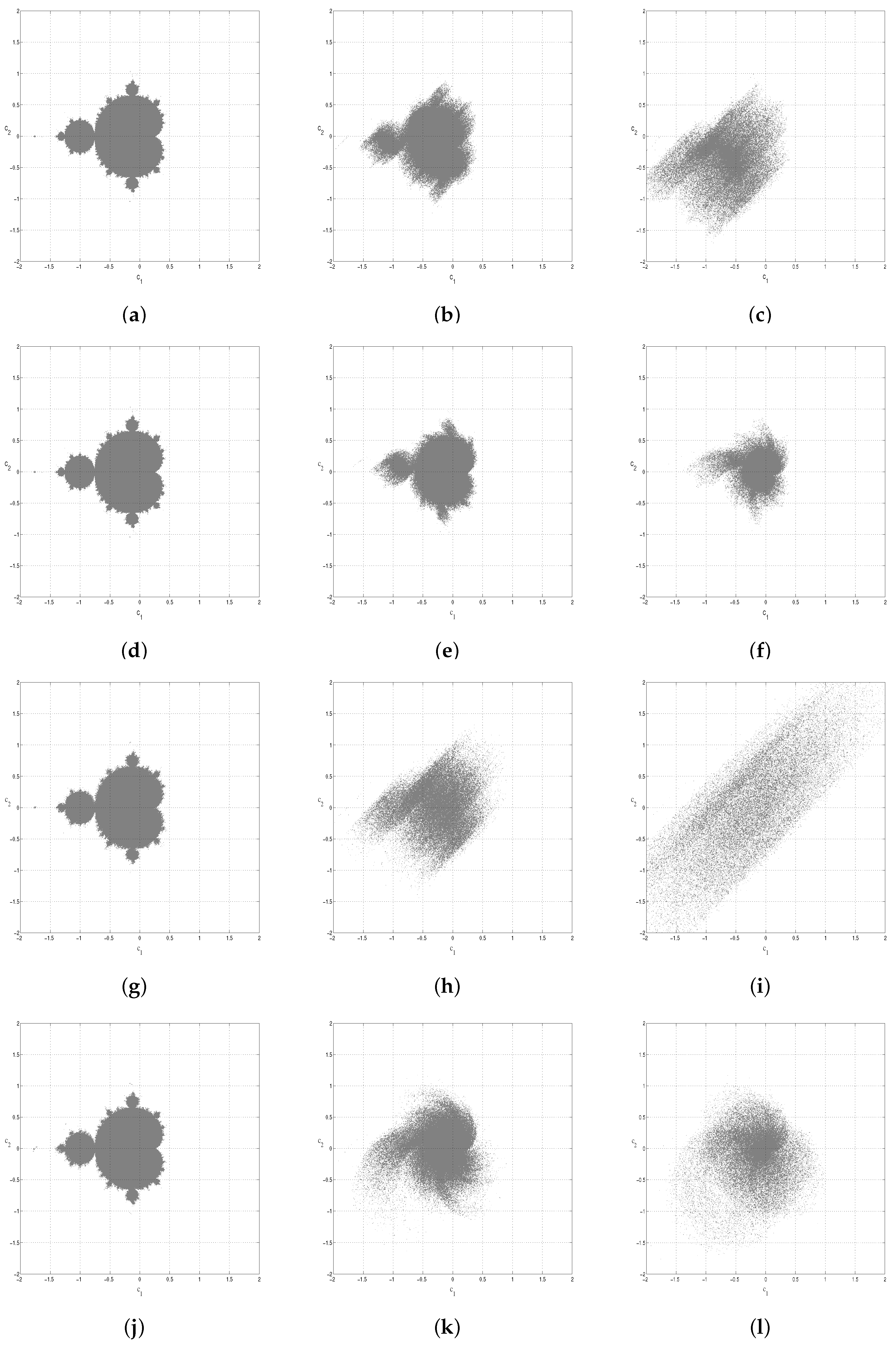
On the basis of the escape-time algorithm, $M\left(f_u^a\right),M\left(f_u^m\right),M\left(f_n^a\right)$, and $M\left(f_n^m\right)$ with different noise strengths a and m are illustrated in Figure 2. At first glance, the symmetrical structure damages become more apparent as the noise strength increases for the four kinds of noises. Otherwise, the additive noise is just like a bomb put inside the original $M\left(f\right)$, while the multiplicative noise has more of a phagocytic effect on $M\left(f\right)$ by destroying it inward from the edge. At last, in terms of destroying the symmetry structure, it seems that the additive noise has a greater effect than the multiplicative noise when $a=m$.

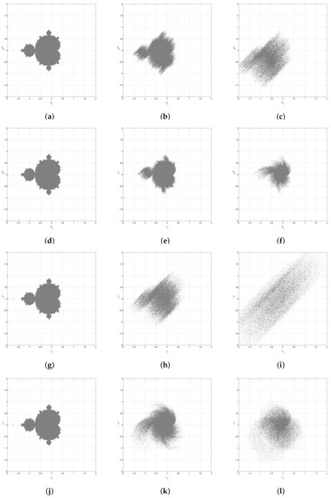
Figure 2. The noise-perturbed Mandelbrot set: (a) $M\left(f_u^{a=0.01}\right)$; (b) $M\left(f_u^{a=0.2}\right)$; (c) $M\left(f_u^{a=0.8}\right)$; (d) $M\left(f_u^{m=0.01}\right)$; (e) $M\left(f_u^{m=0.2}\right)$; (f) $M\left(f_u^{m=0.8}\right)$; (g) $M\left(f_n^{a=0.01}\right)$; (h) $M\left(f_n^{a=0.2}\right)$; (i) $M\left(f_n^{a=0.8}\right)$; (j) $M\left(f_n^{m=0.01}\right)$; (k) $M\left(f_n^{m=0.2}\right)$; (l) $M\left(f_n^{m=0.8}\right)$.

In the following section, a quantified analysis of the above-mentioned observations is given.

3. Methods

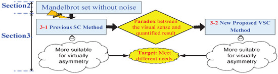
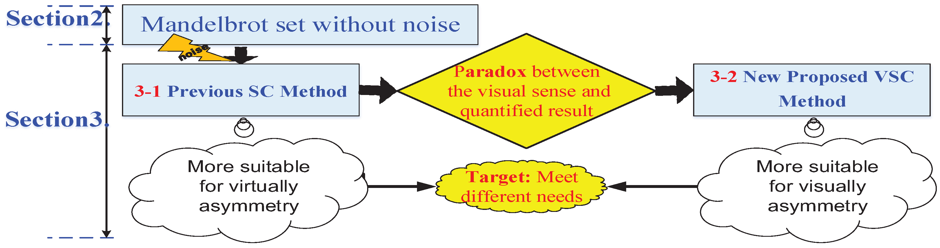
This section contains our main results of quantifying the effect of noises on the symmetry change in the Mandelbrot set. The “symmetry criterion” method [30] was proposed for the analysis of the noise-perturbed Julia set. Here, we modify it so that it is applicable to the study of the noise-perturbed M-set. Figure 3 illustrates the flowchart of Section 2 and Section 3. In this section, the two methods are both realized by the software MATLAB 2014a. The detailed analysis of Figure 3 can be seen in the following two subsections.

Figure 3. The flowchart of Section 2 and Section 3. $SC$, Symmetry Criterion; $VSC$, Visual Symmetry Criterion.

3.1. The “Symmetry Criterion” Method

First, the two parts of the lattice L divided by the $c_1$-axis are respectively denoted by $L_{+}$ (the initial $c_2>0$) and $L_{-}$ (the initial $c_2<0$). For any two initial points ${\mu }_0\in L_{+}$ and ${\nu }_0\in L_{-}$ that are symmetric about the $c_1$-axis, the“symmetry index” [30] is defined as:

$$sy{m}_{c_1}({\mu }_0,{\nu }_0)=\left\{\begin{array}{c}2,if|f^N(x_0,y_0,{\mu }_0)|<Rand|f^N(x_0,y_0,{\nu }_0)|<R.\hfill \\ 0,\left\{\begin{array}{c}if|f^N(x_0,y_0,{\mu }_0)|<Rand|f^N(x_0,y_0,{\nu }_0)|\ge R.\\ if|f^N(x_0,y_0,{\mu }_0)|\ge Rand|f^N(x_0,y_0,{\nu }_0)|<R.\\ if|f^N(x_0,y_0,{\mu }_0)|\ge Rand|f^N(x_0,y_0,{\nu }_0)|\ge R.\end{array}\right.\hfill \end{array}\right.$$

Then, taking $M\left(f_u^a\right)$ as an example, for a given noise strength $a=a_0$, the “symmetry criterion” of $M\left(f_u^a\right)$ about the $c_1$-axis, denoted by $S{C}_{c_1}\left(f_u^{a_0}\right)$, is calculated as follows:

$$\begin{array}{c}S{C}_{c_1}\left(f_u^{a_0}\right)=\frac{1}{num\left(M\left(f_u^{a_0}\right)\right)}\sum _L\left(sy{m}_{c_1}({\mu }_0,{\nu }_0)\right)\hfill \end{array}$$

where $num\left(M\left(f_u^{a_0}\right)\right)$ is the total number of points in $M\left(f_u^{a_0}\right)$ ($num(M\left(f_u^{a_0}\right)$) and can be calculated by the “Julia deviation distance” method [28,29,30]). It is clear that ${\displaystyle \sum _L}(sy{m}_{c_1}({\mu }_0,{\nu }_0)$ is the number of symmetric points in $M\left(f_u^{a_0}\right)$. Thus, $S{C}_{c_1}\left(f_u^{a_0}\right)$ changes in the range of $[0,1]$. The closer that $S{C}_{c_1}\left(f_u^{a_0}\right)$ is to one, the more symmetrical the structure $M\left(f_u^{a_0}\right)$.

Finally, after calculating all the values of $S{C}_{c_1}\left(f_u^{a_0}\right)$ for $a_0\in [0,1]$ in increments of $0.01$, the changing curve of $S{C}_{c_1}\left(f_u^a\right)$ is obtained. The detailed process is omitted for the other three cases, $M\left(f_n^a\right)$, $M\left(f_u^m\right)$, and $M\left(f_n^m\right)$ (we denote both the parameters a and m simply by $\alpha$).

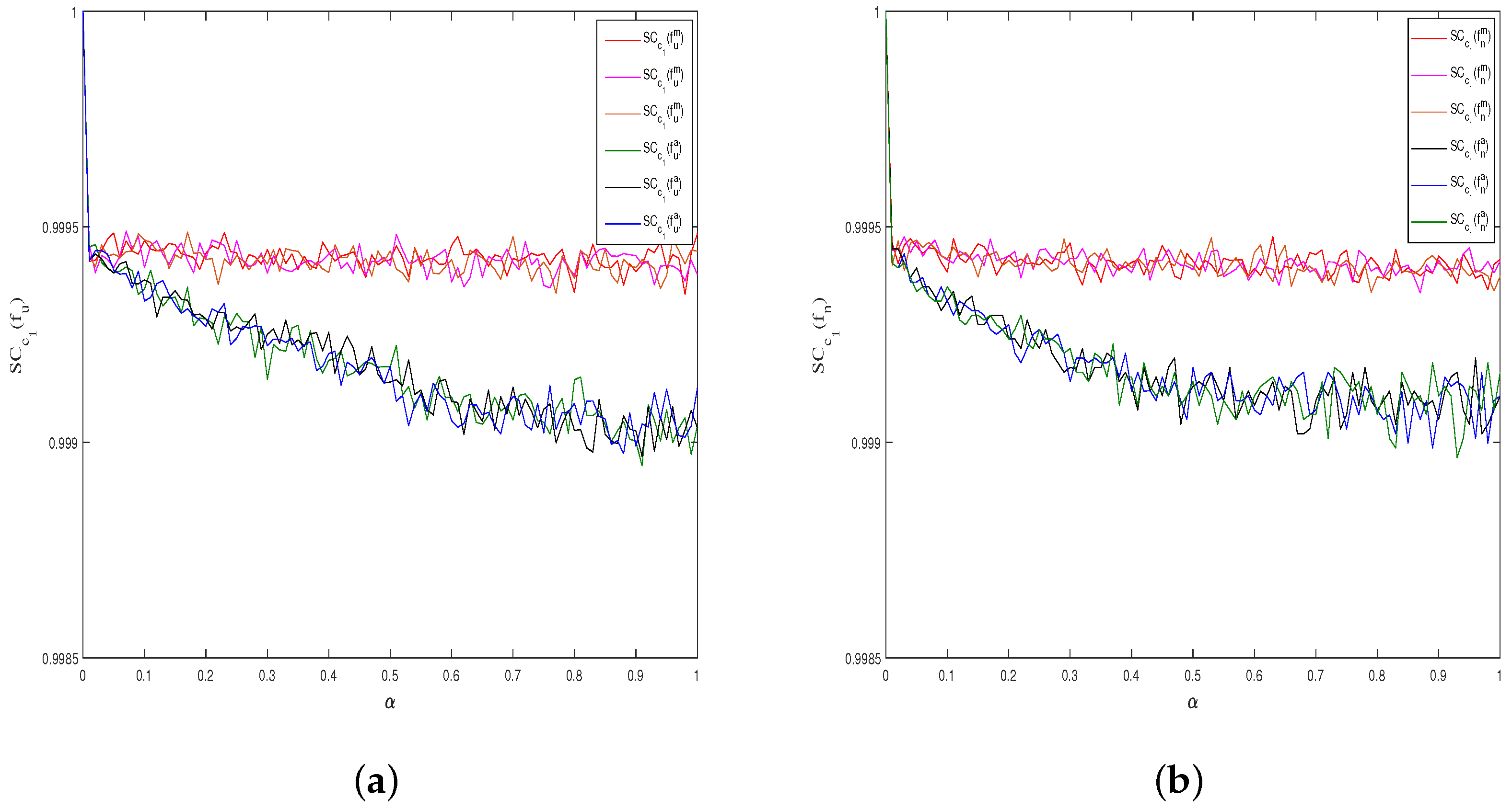
With the above method, we use different colors to depict the three groups of $SC$ curves with $w_n\sim \mathcal{U}(0,1)$ in Figure 4a and $SC$ curves with $w_n\sim \mathcal{N}(0,1)$ in Figure 4b. The three groups’ curves seem to conform to the same statistical law, which can be summarized as follows:

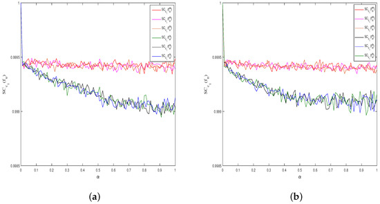
Figure 4. (a) The $S{C}_{c_1}\left(f\right)$ curve with $w_n\sim \mathcal{U}(0,1)$ as the strength of noise increases: additive noise is represented by cool colors, and multiplicative noise is represented by warm colors. (b) The $S{C}_{c_1}\left(f\right)$ curve with $w_n\sim \mathcal{N}(0,1)$ as the strength of noise increases: additive noise is represented by cool colors, and multiplicative noise is represented by warm colors.

(1)

For both $w_n\sim \mathcal{U}(0,1)$ and $w_n\sim \mathcal{N}(0,1)$, the symmetry of $M\left(f^m\right)$ decreases significantly when $m<0,01$, and it tends to be stable on the whole. This observation is in accordance with the conclusion for 3D Julia sets [30].

(2)

For both $w_n\sim \mathcal{U}(0,1)$ and $w_n\sim \mathcal{N}(0,1)$, the symmetry of $M\left(f^a\right)$ decreases with the increase in a, and it continues this trend on the whole.

(3)

For both $w_n\sim \mathcal{U}(0,1)$ and $w_n\sim \mathcal{N}(0,1)$, it can be seen that $S{C}_{c_1}\left(f^a\right)$ is larger than $S{C}_{c_1}\left(f^m\right)$ with the same noise strength $\alpha$. This supports the conclusion in Figure 2.

(4)

Figure 4a,b seems to have roughly the same trend. That is, with the same noise strength, the noises $w_n\sim \mathcal{U}(0,1)$ and $w_n\sim \mathcal{N}(0,1)$ have the same quantized symmetry criterion. A small difference in the details is that the fluctuation of $S{C}_{c_1}\left(f_n^a\right)$ is bigger than that of $S{C}_{c_1}\left(f_u^a\right)$ when $a>0.7$. The visual evidence of this fluctuation can be seen from Figure 2i, in which $M\left(f_n^{a=0.8}\right)$ has almost lost its fractal structure.

(5)

Both $S{C}_{c_1}\left(f_u\right)$ and $S{C}_{c_1}\left(f_n\right)$ remain at a value close to one. That is, the visually-asymmetric noise-perturbed Mandelbrot set may have a high quantified symmetry index.

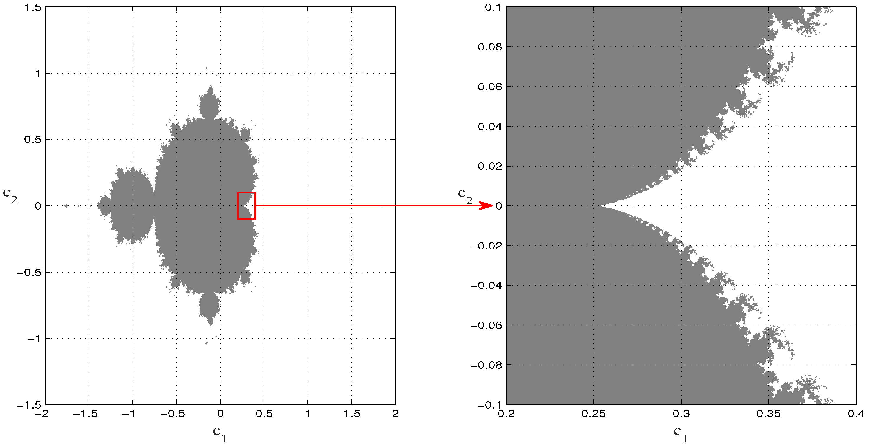
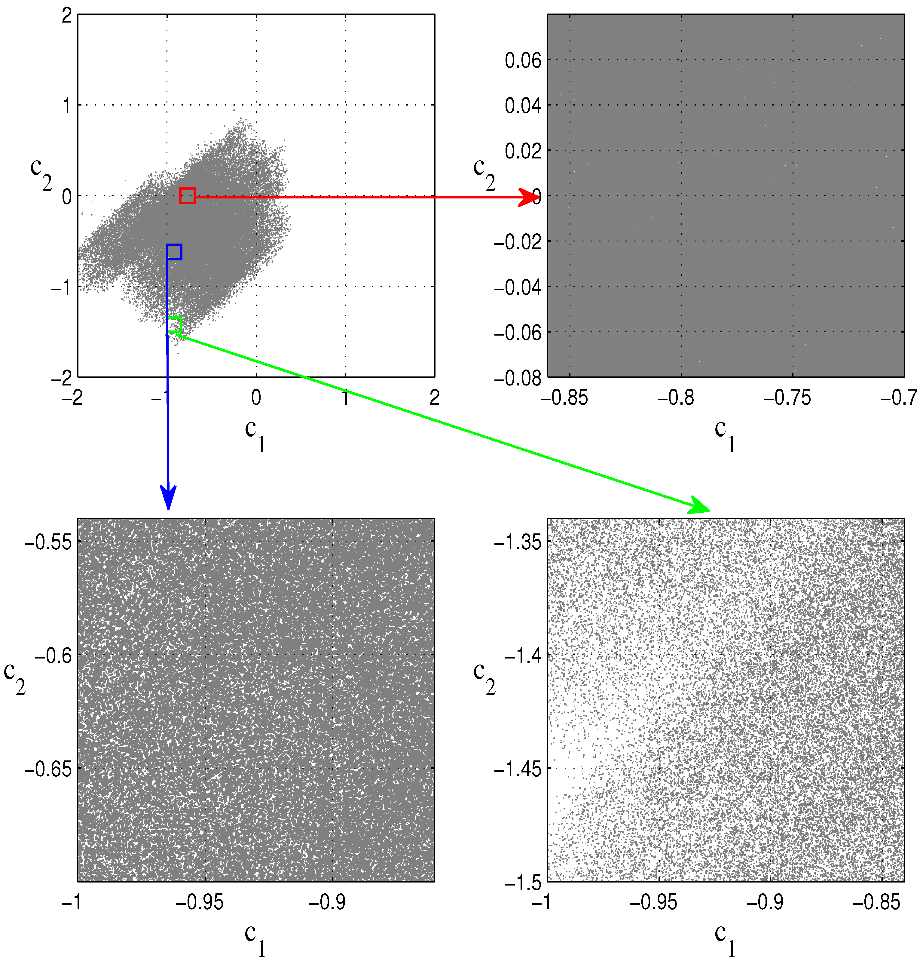
The summary in Section 3.1 in the above list reveals a paradox between the symmetry in the visual sense and the quantified result. We illustrate the partially-enlarged details of $M\left(f^{a=0.8}\right)$ in Figure 5. The results show that the core positions of noise-perturbed M-sets remain dense while the edge positions become relatively sparse. Thus, the higher the resolution of P we choose, the more accurate and bigger the symmetry criterion we obtain.

Figure 5. $M\left(f_u^{a=0.8}\right)$ and three partially-enlarged details of it.

3.2. The Modified “Visual Symmetry Criterion” Method

The paradox mentioned above motivates us to put forward a more effective method to classify the visually-asymmetric fractal set and the virtually-asymmetric fractal set. In terms of the visual sense of symmetry, the edge positions of the fractal set have a stronger visual impact than the core positions. In other words, the weight of $S{C}_{c_1}$ of the points in the edge region should be bigger than the weight of $S{C}_{c_1}$ of the points in the core region. In Figure 2, most of the noise-perturbed M-set remains in $[-1.5,1.5]$ on the $c_2$-axis. Thus, the proper weight of $S{C}_{c_1}$, denoted by w, can be calculated as $w=\frac{\left|img\right({\mu }_0\left)\right|}{1.5}$ ($\left|img\right(·\left)\right|$ means the absolute value of the imaginary part, that is the distance from the axis of symmetry). Then, taking $M\left(f_u^a\right)$ as an example, the modified visual symmetry criterion method is given as follows.

For each point ${\alpha }_0$ in the lattice L, the count index $count\left({\alpha }_0\right)$ is defined as:

$$count\left({\alpha }_0\right)=\left\{\begin{array}{c}w,if|f^N(x_0,y_0,{\alpha }_0)|<R.\hfill \\ 0,if|f^N(x_0,y_0,{\alpha }_0)|\ge R.\hfill \end{array}\right.$$

For any two initial points ${\mu }_0\in L_{+}$ and ${\nu }_0\in L_{-}$ that are symmetric about the $c_1$-plane, the“visual symmetry index” is defined as:

$$sy{m}_{c_1}^{Vis}({\mu }_0,{\nu }_0)=\left\{\begin{array}{c}2w,if|f^N(x_0,y_0,{\mu }_0)|<Rand|f^N(x_0,y_0,{\nu }_0)|<R.\hfill \\ 0,othercases(sameas“symmetrycriterionmetho{d}^{”}).\hfill \end{array}\right.$$

Then, the “visual symmetry criterion” of $M\left(f_u^a\right)$ about the $c_1$-axis, denoted by $S{C}_{c_1}^{Vis}\left(f_u^{a_0}\right)$, is calculated as follows:

$$\begin{array}{c}S{C}_{c_1}^{Vis}\left(f_u^{a_0}\right)=\frac{1}{{\displaystyle \sum _L}\left(count\left({\alpha }_0\right)\right)}\sum _L\left(sy{m}_{c_1}^{Vis}({\mu }_0,{\nu }_0)\right)\hfill \end{array}$$

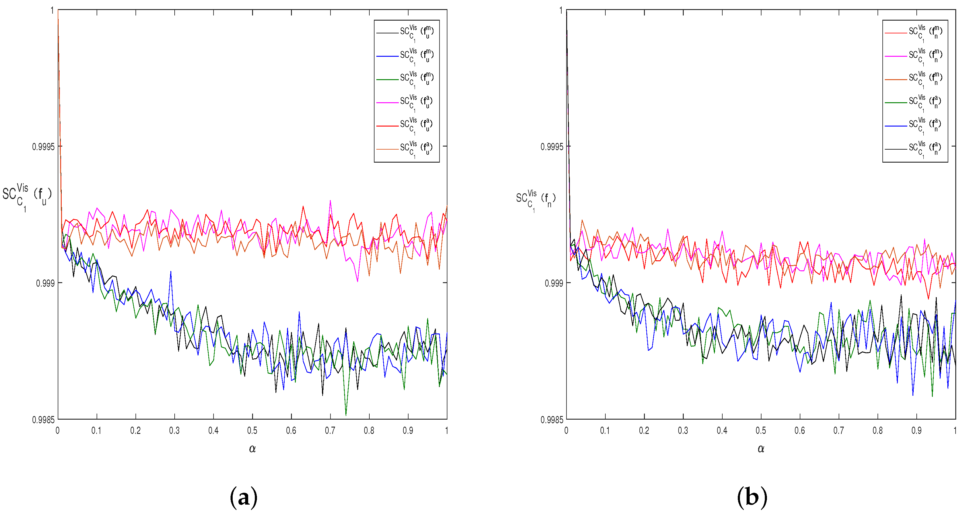
As in the previous subsection, after calculating all the values of $S{C}_{c_1}^{Vis}\left(f^{{\alpha }_0}\right)$ for ${\alpha }_0\in [0,1]$ in increments of $0.01$, the changing curves are determined, as illustrated in Figure 6.

Figure 6. (a) The $S{C}_{c_1}^{Vis}\left(f\right)$ curve with $w_n\sim \mathcal{U}(0,1)$ as the strength of the noise increases: additive noise is represented by cool colors, and multiplicative noise is represented by warm colors. (b) The $S{C}_{c_1}^{Vis}\left(f\right)$ curve with $w_n\sim \mathcal{N}(0,1)$ as the strength of the noise increases: additive noise is represented by cool colors, and multiplicative noise is represented by warm colors.

As shown in Figure 6, for the four cases, $S{C}_{c_1}^{Vis}\left(f\right)$ is bigger than $S{C}_{c_1}\left(f\right)$. Moreover, it can be seen that $S{C}_{c_1}^{Vis}\left(f_n^m\right)$ (see Figure 2d–f) is a little bit bigger than $S{C}_{c_1}^{Vis}\left(f_u^m\right)$ (see Figure 2j–l;). The results illustrate that the modified visual symmetry criterion $S{C}^{Vis}$ is more in line with visual habits.

4. Discussion

The main features of the “symmetry criterion” method [30] and the “Visual Symmetry Criterion” method ($VSC$) proposed in this work can be summarized as follows:

(1)

“Symmetry criterion”: The $SC$ method [30] focuses on the essence of the symmetry distribution. It can be seen in Figure 5 that the region with the dense distribution has a greater effect on the $SC$ results than the region with the sparse distribution. Thus, we can also title the $SC$ method the “virtual symmetry criterion”. It can be applied to engineering problems that require high data accuracy.

(2)

“Visual symmetry criterion”: The $VSC$ method focuses more on the sense of vision. That is, the farther away from the symmetry axis, the greater the effect on the visual sense. Thus, the “visual symmetry criterion” can be applied to some pattern recognition fields that focus on the senses of human beings.

Compared with previous investigations, the novelties of this work can be briefly summarized as follows:

(1)

References [21,22,25,26,27,29] mainly discussed the deviation distance or the structural damages in noise-perturbed fractals sets. Some scholars have examined the symmetry property of noise-perturbed fractal sets [23,24,28], but quantitative investigations of symmetry in a noise-perturbed fractal set are limited to [30] and this work.

(2)

We introduce more types of noise, $w_n\sim \mathcal{U}(0,1)$ and $w_n\sim \mathcal{N}(0,1)$, into such kinds of research.

(3)

A more effective method, the “visual symmetry criterion” method, for classifying the visually-asymmetric set is proposed in this work.

It is noted that graphical exploration is a common method in research on stochastic fractal systems. Thus, the current limitations of this work are summarized as follows:

(1)

The underlying mathematical proof of the graphical and algorithm observations is difficult to provide. We intend to investigate this topic in future work.

(2)

The calculation quantity of the “visual symmetry criterion” is large because it needs to calculate a weight w for each step. Thus, it is hard to extend this method to the spatial case.

5. Conclusions

The present paper demonstrates that the symmetry of the noise-perturbed M-set can be measured in two ways: (1) on the basis of the virtual density distribution and (2) on the basis of the visual sense. As mentioned in the Introduction, since the Mandelbrot set is widely applied in other areas, the $SC$ method and $VSC$ method in this work may have some potential applications in diverse problems. For instance, can the evolution of a population remain stable with the occurrence of environmental changes [14]? Can an encrypted image still be decrypted in the presence of signal interference in the transmission process [15]? Can the networks described by fractals systems remain symmetry with the occurrence of network interference [31,32]. We hope that the preliminary algorithm results in this work can provide insight into the applications mentioned above.

References

- Julia, G. Mèmoire sur l’itèration des fonctions rationnelles. J. Math. Pures Appl. 1918, 8, 47–245. [Google Scholar]
- Mandelbrot, B.B. Fractals and Chaos: The Mandelbrot Set and Beyond; Springer Science & Business Media: New York, NY, USA, 2013; 320p, ISBN 0-387-20158-0. [Google Scholar]
- Lei, T. Similarity between the Mandelbrot set and Julia sets. Commun. Math. Phys. 1990, 134, 587–617. [Google Scholar] [CrossRef]
- Wang, X.Y. Fractal structures of the non-boundary region of the generalized Mandelbrot set. Prog. Nat. Sci. 2001, 11, 693–700. [Google Scholar]
- Liu, S.; Pan, Z.; Fu, W.; Cheng, X. Fractal generation method based on asymptote family of generalized Mandelbrot set and its application. J. Nonlinear Sci. Appl. 2017, 10, 1148–1161. [Google Scholar] [CrossRef]
- Wang, X.; Jin, T. Hyperdimensional generalized M-J sets in hypercomplex number space. Nonlinear Dyn. 2013, 73, 843–852. [Google Scholar] [CrossRef]
- Fisher, Y.; McGuire, M.; Voss, R.F.; Barnsley, M.F.; Devaney, R.L.; Mandelbrot, B.B. The Science of Fractal Images; Peitgen, H.O., Saupe, D., Eds.; Springer Publishing Company, Incorporated: Berlin, Germany, 2011. [Google Scholar]
- Zhang, Y.P.; Sun, W.H. Synchronization and coupling of Mandelbrot sets. Nonlinear Dyn. 2011, 64, 59–63. [Google Scholar] [CrossRef]
- Wang, D.; Liu, S.T.; Zhao, Y.; Jiang, C.M. Control of the spatial Mandelbrot set generated in coupled map lattice. Nonlinear Dyn. 2016, 84, 1795–1803. [Google Scholar] [CrossRef]
- Rani, M.; Kumar, V. Superior Mandelbrot set. J. Korea Soc. Math. Educ. Ser. D Res. Math. Educ. 2004, 8, 279–291. [Google Scholar]
- Rochon, D. A generalized Mandelbrot set for bicomplex numbers. Fractals 2010, 8, 355–368. [Google Scholar] [CrossRef]
- Beck, C. Physical meaning for Mandelbrot and Julia sets. Phys. Nonlinear Phenom. 1999, 125, 171–182. [Google Scholar] [CrossRef]
- Levin, M. Morphogenetic fields in embryogenesis, regeneration, and cancer: Non-local control of complex patterning. Biosystems 2012, 109, 243–261. [Google Scholar] [CrossRef] [PubMed]
- Sun, W.H.; Zhang, Y.P. Fractal analysis and control in the predator-prey model. Int. J. Comput. Math. 2017, 94, 737–746. [Google Scholar] [CrossRef]
- Sun, Y.; Xu, R.; Chen, L.; Xu, X. Image compression and encryption scheme using fractal dictionary and Julia set. Image Process. IET 2014, 9, 173–183. [Google Scholar] [CrossRef]
- Butusov, D.N.; Karimov, A.I.; Pyko, N.S.; Pyko, S.A.; Bogachev, M.I. Discrete chaotic maps obtained by symmetric integration. Phys. Stat. Mech. Its Appl. 2018, 509, 955–970. [Google Scholar] [CrossRef]
- Butusov, D.N.; Karimov, A.I.; Tutueva, A.V. Symmetric extrapolation solvers for ordinary differential equations. In Proceedings of the 2016 IEEE NW Russia Young Researchers in Electrical and Electronic Engineering Conference, St. Petersburg, Russia, 2–3 February 2016; pp. 162–167. [Google Scholar]
- Li, C.; Hu, W.; Sprott, J.C.; Wang, X. Multistability in symmetric chaotic systems. Eur. Phys. J. Spec. Top. 2015, 224, 1493–1506. [Google Scholar] [CrossRef]
- Bandt, C. On the Mandelbrot set for pairs of linear maps. Nonlinearity 2002, 15, 11–27. [Google Scholar] [CrossRef]
- Wang, D.; Liu, S.T. On the boundedness and symmetry properties of the fractal sets generated from alternated complex map. Symmetry 2016, 8, 7. [Google Scholar] [CrossRef]
- Argyris, J.; Karakasidis, T.E.; Andreadis, I. On the Julia set of the perturbed Mandelbrot map. Chaos Solitons Fractals 2000, 11, 2067–2073. [Google Scholar] [CrossRef]
- Argyris, J.; Karakasidis, T.E.; Andreadis, I. On the Julia sets of a noise-perturbed Mandelbrot map. Chaos Solitons Fractals 2002, 13, 245–252. [Google Scholar] [CrossRef]
- Argyris, J.; Andreadis, I.; Karakasidis, T.E. On perturbations of the Mandelbrot map. Chaos Solitons Fractals 2000, 11, 1131–1136. [Google Scholar] [CrossRef]
- Wang, X.Y.; Wang, Z.; Lang, Y.; Zhang, Z.F. Noise perturbed generalized Mandelbrot sets. J. Math. Anal. Appl. 2008, 347, 179–187. [Google Scholar] [CrossRef]
- Wang, X.Y.; Jia, R.H.; Zhang, Z.F. The generalized Mandelbrot set perturbed by composing noise of additive and multiplicative. Appl. Math. Comput. 2009, 210, 107–118. [Google Scholar]
- Rani, M.; Agarwal, R. Effect of stochastic noise on superior Julia sets. J. Math. Imaging Vis. 2010, 36, 63. [Google Scholar] [CrossRef]
- Agarwal, R.; Agawal, V. Dynamic noise perturbed generalized superior Mandelbrot sets. Nonlinear Dyn. 2012, 67, 1883–1891. [Google Scholar] [CrossRef]
- Andreadis, I.; Karakasidis, T.E. On a topological closeness of perturbed Mandelbrot sets. Appl. Math. Comput. 2010, 215, 3674–3683. [Google Scholar] [CrossRef]
- Andreadis, I.; Karakasidis, T.E. On a closeness of the Julia sets of noise-perturbed complex quadratic maps. Int. J. Bifurc. Chaos 2012, 22, 1250221. [Google Scholar] [CrossRef]
- Wang, D.; Liu, X.Y. On the noise-perturbed spatial Julia set generated by Lorenz system. Commun. Nonlinear Sci. Numer. Simul. 2017, 50, 229–240. [Google Scholar] [CrossRef]
- Rădulescu, A.; Pignatelli, A. Real and complex behavior for networks of coupled logistic maps. Nonlinear Dyn. 2017, 87, 1295–1313. [Google Scholar]
- Rădulescu, A.; Evans, S. Asymptotic sets in networks of coupled quadratic nodes. J. Complex Netw. 2018. [Google Scholar] [CrossRef]
© 2019 by the authors. Licensee MDPI, Basel, Switzerland. This article is an open access article distributed under the terms and conditions of the Creative Commons Attribution (CC BY) license (http://creativecommons.org/licenses/by/4.0/).