Stereo Matching Methods for Imperfectly Rectified Stereo Images


Abstract
:1. Introduction
2. Matching Cost Functions
2.1. Application to Dense Stereo Matching
2.2. Application to Pixel-Wise Matching Cost Functions
2.2.1. ImpAD
2.2.2. ImpSD
2.3. Application to Transform-Based Matching Cost Functions
2.3.1. ImpRank
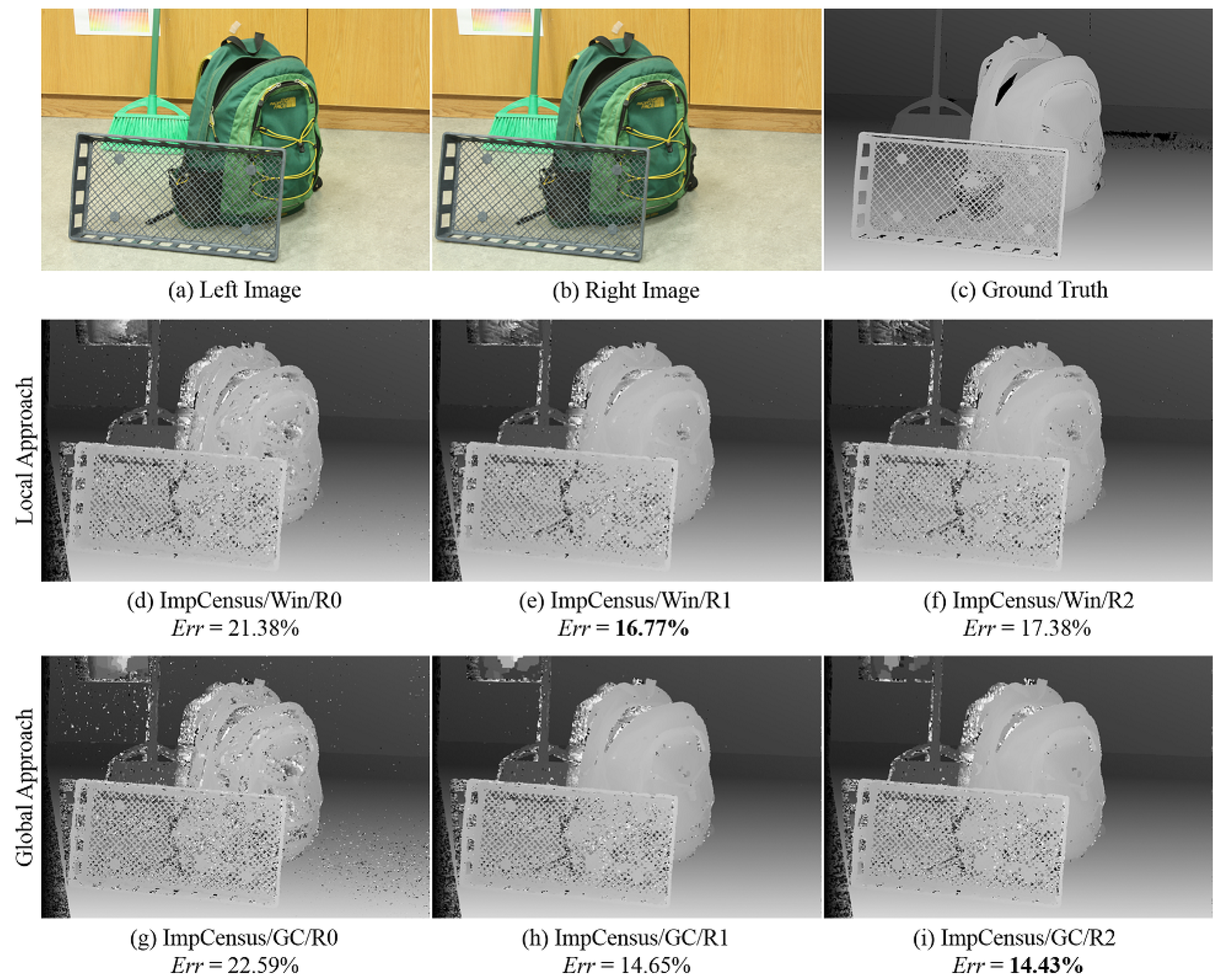
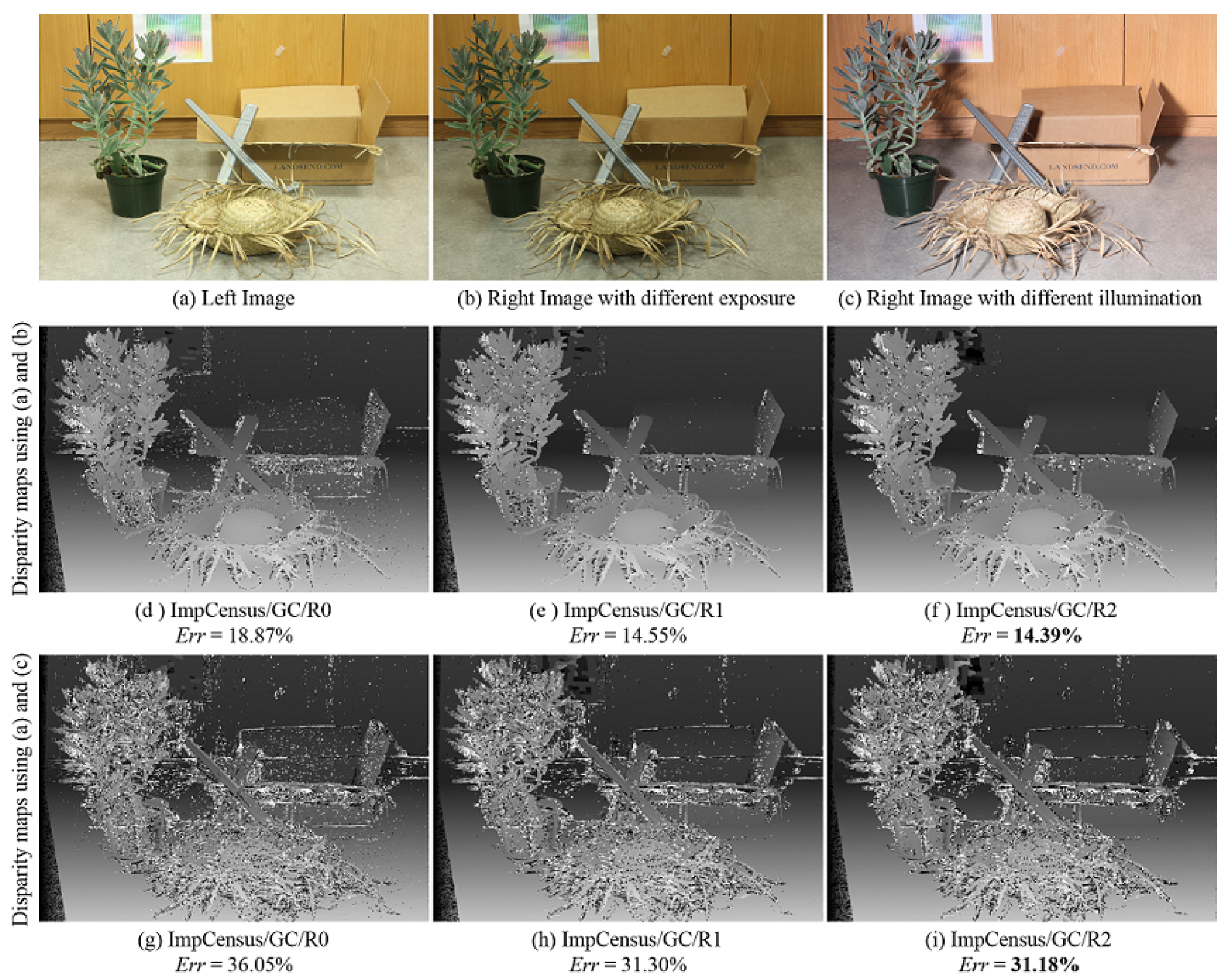
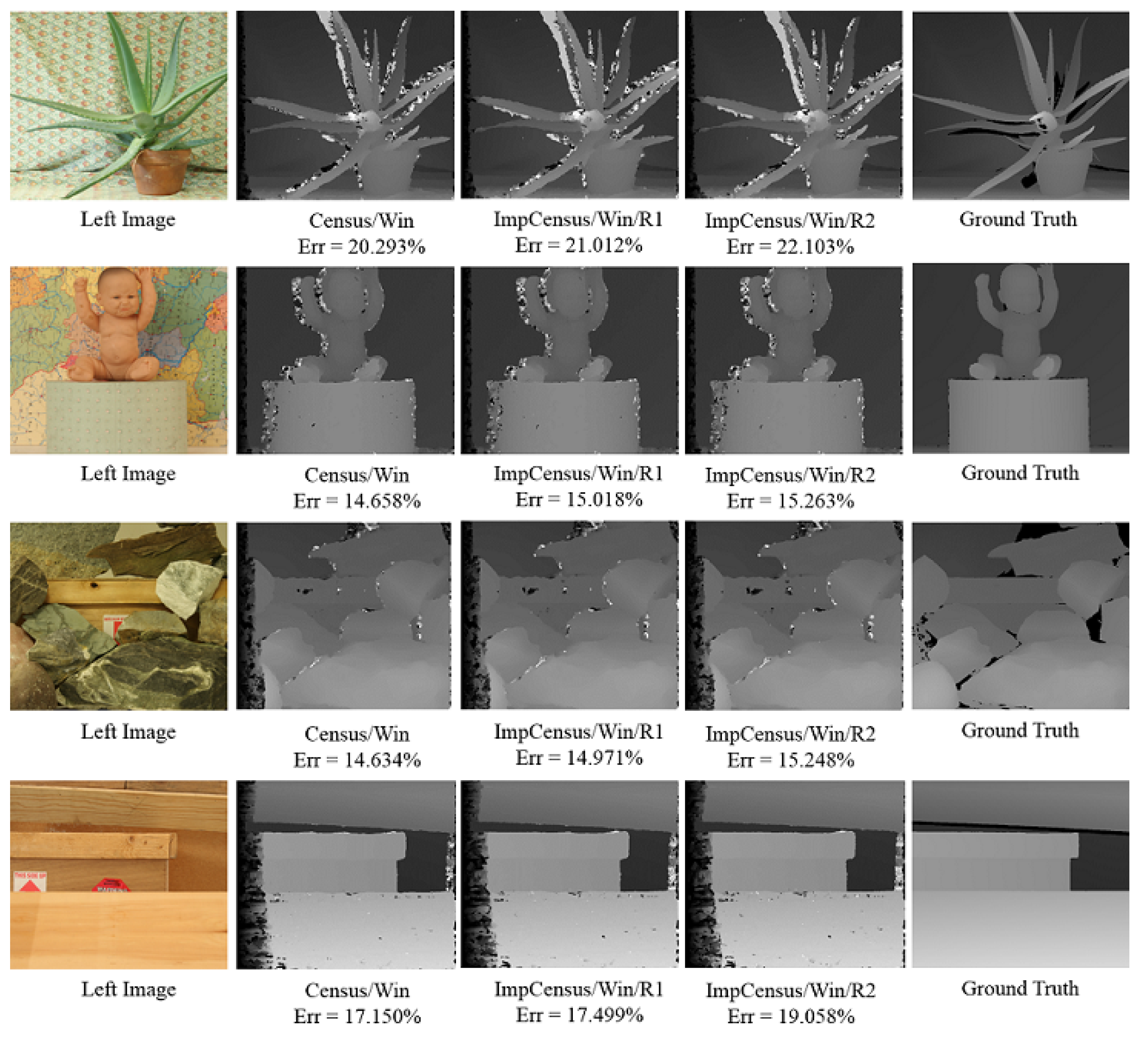
2.3.2. ImpCensus
2.4. Application to Window-Based Matching Cost Functions
2.4.1. ImpNCC
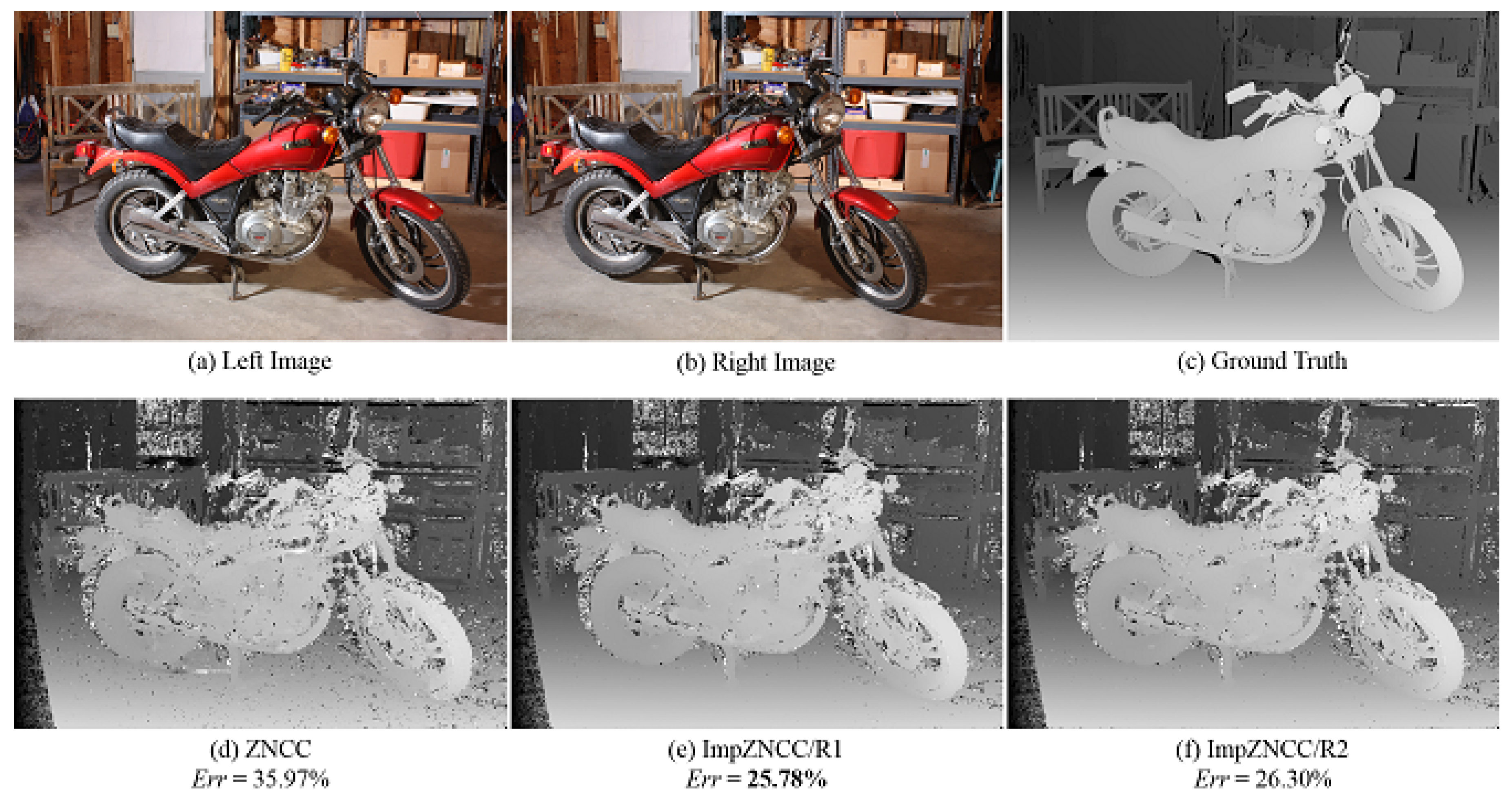
2.4.2. ImpZNCC
| Algorithm 1 The procedure of ImpZNCC matching cost function to construct . |
| Input: Left and right images I and , window size W, expansion range R. compute average over W for I using BF compute average over W for using BF compute sum over W for using BF compute sum over W for using BF For to do For to R do compute sum over W from using BF compute end for end for Return |
3. Experimental Results
3.1. ImpCensus and ImpRank
3.2. ImpAD and ImpSD
3.3. ImpNCC and ImpZNCC
3.4. Stereo Image with Radiometric Distortion
3.5. Using Normal Stereo Images
3.6. Computation Time
4. Conclusions
Author Contributions
Funding
Conflicts of Interest
References
- Trucco, E.; Verri, A. Introductory Techniques For 3-D Computer Vision; Prentice Hall PTR: Upper Saddle River, NJ, USA, 1998. [Google Scholar]
- Cyganek, B.; Siebert, J.P. Introduction to 3D Computer Vision Techniques and Algorithms; Wiley: Hoboken, NJ, USA, 2009. [Google Scholar]
- Meister, S.; Jähne, B.; Kondermann, D. Outdoor stereo camera system for the generation of real-world benchmark data sets. Opt. Eng. 2012, 51, 021107. [Google Scholar] [CrossRef]
- Geiger, A.; Lenz, P.; Urtasun, R. Are we ready for Autonomous Driving? The KITTI Vision Benchmark Suite. In Proceedings of the 2012 IEEE Conference on Computer Vision and Pattern Recognition, Providence, RI, USA, 16–21 June 2012. [Google Scholar]
- Lowe, D.G. Distinctive Image Features from Scale-Invariant Keypoints. Int. J. Comput. Vis. 2004, 60, 91–110. [Google Scholar] [CrossRef]
- Bay, H.; Tuytelaars, T.; Van Gool, L. SURF: Speeded Up Robust Features. In Proceedings of the Ninth European Conference on Computer Vision, Graz, Austria, 7–13 May 2006. [Google Scholar]
- Medioni, G.; Nevatia, R. Segment-based stereo matching. Comput. Vis. Graph. Image Process. 1985, 31, 2–18. [Google Scholar] [CrossRef]
- Robert, L.; Faugeras, O. Curve-based stereo: Figural continuity and curvature. In Proceedings of the IEEE Conference on Computer Vision and Pattern Recognition, Lahaina, HI, USA, 3–6 June 1991. [Google Scholar]
- Olson, C.F. Subpixel localization and uncertainty estimation using occupancy grids. In Proceedings of the IEEE International Conference on Robotics and Automation, Detroit, MI, USA, 10–15 May 1999. [Google Scholar]
- Sarkis, M.; Diepold, K. Sparse stereo matching using belief propagation. In Proceedings of the IEEE International Conference on Image Processing, San Diego, CA, USA, 12–15 October 2008. [Google Scholar]
- Geiger, A.; Roser, M.; Urtasun, R. Efficient Large-Scale Stereo Matching. In Proceedings of the Asian Conference on Computer Vision (ACCV), Queenstown, New Zealand, 8–12 November 2010. [Google Scholar]
- Scharstein, D.; Szeliski, R. A taxonomy and evaluation of dense two-frame stereo correspondence algorithms. Int. J. Comput. Vis. 2002, 47, 7–42. [Google Scholar] [CrossRef]
- Kolmogorov, V.; Zabih, R.R. Computing Visual Correspondence with Occlusions using Graph Cuts. Proc. ICCV 2001, 2, 508–515. [Google Scholar]
- Felzenszwalb, P.F.; Huttenlocher, D.P. Efficient Belief Propagation for Early Vision. Int. J. Comput. Vis. 2006, 70, 41–54. [Google Scholar] [CrossRef]
- Hirschmuller, H.; Scharstein, D. Evaluation of stereo matching costs on images with radiometric differences. IEEE Trans. Pattern Anal. Mach. Intell. 2009, 31, 1582–1599. [Google Scholar] [CrossRef] [PubMed]
- Nguyen, V.D.; Nguyen, D.D.; Nguyen, T.T.; Dinh, V.Q.; Jeon, J.W. Support local pattern and its application to disparity improvement and texture classification. IEEE Trans. Circuits Syst. Video Technol. 2014, 24, 263–276. [Google Scholar] [CrossRef]
- Heo, Y.S.; Lee, K.M.; Lee, S.U. Robust Stereo Matching Using Adaptive Normalized Cross-Correlation. IEEE Trans. Pattern Anal. Mach. Intell. 2011, 33, 807–822. [Google Scholar] [PubMed]
- Hosni, A.; Rhemann, C.; Bleyer, M.; Rother, C.; Gelautz, M. Fast Cost-Volume Filtering for Visual Correspondence and Beyond. IEEE Trans. Pattern Anal. Mach. Intell. 2013, 35, 504–511. [Google Scholar] [CrossRef] [PubMed]
- Scharstein, D.; Hirschmüller, H.; Kitajima, Y.; Krathwohl, G.; Nesic, N.; Wang, X.; Westling, P. High-resolution stereo datasets with subpixel-accurate ground truth. Conf. Pattern Recognit. 2014. [Google Scholar] [CrossRef]
- Wang, Y.; Wang, K.; Dunn, E.; Frahm, J.-M. Stereo under sequential optimal sampling: A statistical analysis framework for search space reduction. In Proceedings of the IEEE Computer Society Conference on Computer Vision and Pattern Recognition, Washington, DC, USA, 23–28 June 2014; pp. 485–492. [Google Scholar]
- Luo, W.; Schwing, A.G.; Urtasun, R. Efficient Deep Learning for Stereo Matching. In Proceedings of the 2016 IEEE Conference on Computer Vision and Pattern Recognition (CVPR), Las Vegas, NV, USA, 27–30 June 2016; pp. 5695–5703. [Google Scholar]
- Kowalczuk, J.; Psota, E.T.; Perez, L.C. Real-Time Stereo Matching on CUDA Using an Iterative Refinement Method for Adaptive Support-Weight Correspondences. IEEE Trans. Circuits Syst. Video Technol. 2013, 23, 94–104. [Google Scholar] [CrossRef]
- Hirschmüller, H.; Innocent, P.R.; Garibaldi, J. Real-Time Correlation-Based Stereo Vision with Reduced Border Errors. Int. J. Comput. Vis. 2002, 47, 229–246. [Google Scholar] [CrossRef]
- Li, L.; Zhang, S.; Yu, X.; Zhang, L. PMSC: PatchMatch-Based Superpixel Cut for Accurate Stereo Matching. IEEE Trans. Circuits Syst. Video Technol. 2018, 28, 679–692. [Google Scholar] [CrossRef]
- Psota, E.T.; Kowalczuk, J.; Mittek, M.; Perez, L.C. MAP Disparity Estimation Using Hidden Markov Trees. IEEE Trans. Circuits Syst. Video Technol. 2018, 28, 2219–2227. [Google Scholar]
- Li, L.; Yu, X.; Zhang, S.; Zhao, X.; Zhang, L. 3D Cost Aggregation with Multiple Minimum Spanning Trees for Stereo Matching. 2017. Available online: http://ao.osa.org/abstract.cfm?URI=ao-56-12-3411 (accessed on 19 April 2019).
- Kim, K.R.; Kim, C.S. Adaptive smoothness constraints for efficient stereo matching using texture and edge information. In Proceedings of the 2016 IEEE International Conference on Image Processing (ICIP), Phoenix, AZ, USA, 25–28 September 2016; pp. 3429–3433. [Google Scholar]
- Nahar, S.; Joshi, M.V. A learned sparseness and IGMRF-based regularization framework for dense disparity estimation using unsupervised feature learning. IPSJ Trans. Comput. Vis. Appl. 2017, 9, 3429–3433. [Google Scholar] [CrossRef]
- Kanade, T.; Kano, H.; Kimura, S.; Yoshida, A.; Oda, K. Development of a video-rate stereo machine. In Proceedings of the 1995 IEEE/RSJ International Conference on Intelligent Robots and Systems, Pittsburgh, PA, USA, 5–9 August 1995. [Google Scholar]
- Antunes, M.; Barreto, J.P. SymStereo: Stereo Matching using Induced Symmetry. Int. J. Comput. Vis. 2014, 109, 187–208. [Google Scholar] [CrossRef]
- McDonnell, M.J. Box-Filtering techniques. Comput. Graph. Image Process. 1981, 17, 65–70. [Google Scholar] [CrossRef]
- Crow, F. Summed-area tables for texture mapping. SIGGRAPH 1984, 18, 207–212. [Google Scholar] [CrossRef]
- Scharstein, D.; Szeliski, R. Middlebury Online Stereo Evaluation. 2002. Available online: http://vision.middlebury.edu/stereo (accessed on 19 April 2019).
- Boykov, Y.; Kolmogorov, V. An Experimental Comparison of Min-Cut/Max-Flow Algorithms for Energy Minimization in Vision. IEEE Trans. Pattern Anal. Mach. Intell. 2004, 26, 1124–1137. [Google Scholar] [CrossRef] [PubMed]
- Kolmogorov, V. Min-Cut/Max-Flow Algorithm Source Code. 2004. Available online: http://pub.ist.ac.at/vnk/software.html (accessed on 19 April 2019).
- Scharstein, D.; Szeliski, R. Middlebury Online Stereo Evaluation. Available online: http://vision.middlebury.edu/stereo/eval3 (accessed on 19 April 2019 ).


| Dataset | Height | Width | Disparity | Dataset | Height | Width | Disparity |
|---|---|---|---|---|---|---|---|
| Adirondack | 1984 | 2872 | 290 | Playroom | 1904 | 2796 | 330 |
| Backpack | 1988 | 2948 | 260 | Playtable | 1852 | 2720 | 290 |
| Bicycle | 1968 | 3052 | 180 | Recycle | 1944 | 2880 | 260 |
| Cable | 1916 | 2816 | 460 | Shelves | 1988 | 2952 | 240 |
| Classroom | 1896 | 2996 | 260 | Storage | 1988 | 2792 | 660 |
| Couch | 1992 | 2296 | 630 | Sword1 | 2004 | 2928 | 260 |
| Flowers | 1984 | 2888 | 640 | Sword2 | 1956 | 2884 | 370 |
| Motorcycle | 1988 | 2964 | 280 | Umbrella | 2008 | 2960 | 250 |
| Pipes | 1940 | 2940 | 300 |
| Local Algorithms | Global Algorithms | ||||||
|---|---|---|---|---|---|---|---|
| Dataset | Census | ImpCensus/R1 | ImpCensus/R2 | Dataset | Census | ImpCensus/R1 | ImpCensus/R2 |
| Adirondack | 45.30 | 38.45 | 37.62 | Adirondack | 52.71 | 37.67 | 31.14 |
| Backpack | 21.38 | 16.77 | 17.38 | Backpack | 22.59 | 14.65 | 14.43 |
| Bicycle | 51.21 | 45.10 | 42.12 | Bicycle | 53.69 | 43.13 | 35.01 |
| Cable | 51.84 | 45.47 | 42.46 | Cable | 63.39 | 47.07 | 36.37 |
| Classroom | 30.41 | 26.89 | 28.45 | Classroom | 38.47 | 25.49 | 18.85 |
| Couch | 30.65 | 29.42 | 30.50 | Couch | 33.34 | 28.05 | 26.83 |
| Flowers | 61.64 | 56.38 | 54.37 | Flowers | 64.70 | 54.43 | 49.27 |
| Motorcycle | 29.50 | 21.63 | 20.62 | Motorcycle | 37.30 | 21.25 | 17.52 |
| Pipes | 33.59 | 28.08 | 25.64 | Pipes | 38.46 | 27.52 | 22.70 |
| Playroom | 45.23 | 43.14 | 43.64 | Playroom | 49.79 | 42.09 | 39.13 |
| Playtable | 65.28 | 39.50 | 37.38 | Playtable | 70.29 | 34.92 | 31.20 |
| Recycle | 44.81 | 40.27 | 40.39 | Recycle | 50.74 | 36.91 | 31.72 |
| Shelves | 54.33 | 48.27 | 48.11 | Shelves | 56.88 | 47.38 | 44.78 |
| Storage | 54.70 | 49.74 | 47.33 | Storage | 63.41 | 51.99 | 44.81 |
| Sword1 | 16.45 | 15.61 | 16.43 | Sword1 | 18.41 | 14.08 | 13.99 |
| Sword2 | 70.24 | 62.97 | 57.66 | Sword2 | 71.63 | 52.73 | 36.92 |
| Umbrella | 66.17 | 63.64 | 64.40 | Umbrella | 70.62 | 62.23 | 56.46 |
| Average | 45.46 | 39.49 | 38.50 | Average | 50.38 | 37.74 | 32.42 |
| Local Algorithms | Global Algorithms | ||||||
|---|---|---|---|---|---|---|---|
| Dataset | Rank | ImpRank/R1 | ImpRank/R2 | Dataset | Rank | ImpRank/R1 | ImpRank/R2 |
| Adirondack | 59.68 | 50.66 | 54.20 | Adirondack | 48.30 | 34.06 | 33.27 |
| Backpack | 25.60 | 20.21 | 24.27 | Backpack | 20.18 | 14.64 | 16.01 |
| Bicycle | 60.81 | 52.77 | 51.79 | Bicycle | 48.57 | 35.77 | 31.24 |
| Cable | 67.54 | 60.01 | 63.09 | Cable | 51.65 | 34.82 | 35.74 |
| Classroom | 41.49 | 38.41 | 48.13 | Classroom | 23.91 | 11.23 | 10.29 |
| Couch | 38.48 | 35.84 | 45.36 | Couch | 30.53 | 27.18 | 32.48 |
| Flowers | 72.03 | 62.64 | 62.66 | Flowers | 60.68 | 48.51 | 46.57 |
| Motorcycle | 43.21 | 29.73 | 31.26 | Motorcycle | 30.47 | 17.86 | 17.55 |
| Pipes | 42.67 | 34.91 | 34.13 | Pipes | 32.96 | 25.24 | 23.51 |
| Playroom | 55.61 | 50.74 | 54.73 | Playroom | 45.05 | 38.27 | 39.77 |
| Playtable | 73.64 | 54.26 | 52.70 | Playtable | 69.88 | 39.36 | 40.49 |
| Recycle | 64.45 | 53.01 | 56.38 | Recycle | 43.92 | 30.58 | 29.46 |
| Shelves | 58.34 | 53.21 | 57.39 | Shelves | 55.57 | 46.56 | 46.75 |
| Storage | 69.30 | 62.34 | 64.56 | Storage | 57.90 | 36.67 | 35.60 |
| Sword1 | 20.71 | 19.07 | 23.50 | Sword1 | 14.08 | 11.57 | 13.80 |
| Sword2 | 78.81 | 75.55 | 77.43 | Sword2 | 63.11 | 44.13 | 39.95 |
| Umbrella | 71.83 | 70.07 | 72.47 | Umbrella | 64.13 | 52.05 | 50.66 |
| Average | 55.54 | 48.44 | 51.41 | Average | 44.76 | 32.26 | 31.95 |
| Local Algorithms | Global Algorithms | ||||||
|---|---|---|---|---|---|---|---|
| Dataset | AD | ImpAD/R1 | ImpAD/R2 | Dataset | AD | ImpAD/R1 | ImpAD/R2 |
| Adirondack | 54.17 | 46.33 | 47.48 | Adirondack | 42.09 | 29.28 | 31.11 |
| Backpack | 28.57 | 22.54 | 24.39 | Backpack | 38.25 | 21.59 | 22.28 |
| Bicycle | 61.27 | 55.25 | 53.39 | Bicycle | 50.68 | 38.03 | 35.97 |
| Cable | 65.63 | 59.14 | 60.25 | Cable | 43.09 | 33.97 | 33.32 |
| Classroom | 40.77 | 38.37 | 44.96 | Classroom | 18.13 | 12.42 | 12.96 |
| Couch | 37.95 | 35.09 | 40.32 | Couch | 33.86 | 30.99 | 33.78 |
| Flowers | 69.47 | 62.56 | 62.35 | Flowers | 59.56 | 52.83 | 47.05 |
| Motorcycle | 41.39 | 28.82 | 28.54 | Motorcycle | 40.81 | 25.01 | 22.64 |
| Pipes | 43.49 | 35.38 | 33.01 | Pipes | 49.42 | 30.39 | 25.62 |
| Playroom | 50.55 | 49.43 | 51.82 | Playroom | 43.44 | 40.26 | 41.67 |
| Playtable | 69.14 | 50.99 | 46.05 | Playtable | 67.20 | 44.29 | 35.48 |
| Recycle | 56.66 | 52.55 | 55.04 | Recycle | 30.53 | 25.90 | 30.18 |
| Shelves | 57.14 | 52.39 | 54.05 | Shelves | 55.84 | 49.21 | 49.84 |
| Storage | 74.25 | 68.04 | 70.28 | Storage | 68.02 | 49.34 | 45.84 |
| Sword1 | 28.13 | 23.65 | 26.50 | Sword1 | 34.18 | 18.98 | 19.63 |
| Sword2 | 76.54 | 73.75 | 74.28 | Sword2 | 54.70 | 42.99 | 36.46 |
| Umbrella | 70.67 | 68.18 | 69.36 | Umbrella | 47.41 | 42.60 | 43.98 |
| Average | 54.46 | 48.38 | 49.53 | Average | 45.72 | 34.59 | 33.40 |
| Local Algorithms | Global Algorithms | ||||||
|---|---|---|---|---|---|---|---|
| Dataset | SD | ImpSD/R1 | ImpSD/R2 | Dataset | SD | ImpSD/R1 | ImpSD/R2 |
| Adirondack | 54.19 | 46.28 | 48.20 | Adirondack | 41.67 | 31.37 | 37.42 |
| Backpack | 29.46 | 23.01 | 25.15 | Backpack | 40.88 | 23.02 | 23.36 |
| Bicycle | 62.21 | 56.31 | 54.57 | Bicycle | 50.23 | 44.38 | 42.52 |
| Cable | 65.30 | 59.24 | 61.41 | Cable | 41.96 | 34.37 | 35.24 |
| Classroom | 40.46 | 38.15 | 41.93 | Classroom | 16.49 | 12.59 | 13.18 |
| Couch | 38.35 | 35.92 | 42.31 | Couch | 34.86 | 32.33 | 36.47 |
| Flowers | 70.10 | 63.60 | 64.52 | Flowers | 56.56 | 44.75 | 51.13 |
| Motorcycle | 42.07 | 29.45 | 29.84 | Motorcycle | 41.33 | 25.47 | 25.17 |
| Pipes | 44.34 | 35.90 | 33.85 | Pipes | 50.06 | 30.97 | 27.12 |
| Playroom | 51.04 | 50.32 | 52.23 | Playroom | 42.66 | 42.39 | 45.01 |
| Playtable | 69.25 | 51.93 | 48.25 | Playtable | 67.74 | 46.73 | 37.77 |
| Recycle | 56.22 | 52.67 | 54.10 | Recycle | 32.77 | 30.59 | 27.42 |
| Shelves | 56.72 | 52.35 | 54.70 | Shelves | 53.70 | 50.51 | 53.21 |
| Storage | 74.35 | 67.51 | 70.09 | Storage | 66.77 | 46.59 | 46.97 |
| Sword1 | 29.97 | 25.11 | 27.80 | Sword1 | 36.40 | 19.40 | 19.93 |
| Sword2 | 76.56 | 73.68 | 74.99 | Sword2 | 51.32 | 41.65 | 38.54 |
| Umbrella | 70.34 | 68.05 | 69.78 | Umbrella | 47.54 | 44.45 | 42.62 |
| Average | 54.76 | 48.79 | 50.22 | Average | 45.47 | 35.39 | 35.47 |
| Dataset | NCC | ImpNCC/R1 | ImpNCC/R2 |
|---|---|---|---|
| Adirondack | 49.40 | 45.22 | 46.11 |
| Backpack | 25.42 | 21.43 | 22.11 |
| Bicycle | 58.23 | 54.09 | 53.12 |
| Cable | 54.85 | 49.64 | 48.51 |
| Classroom | 43.38 | 41.67 | 43.37 |
| Couch | 35.10 | 35.34 | 36.11 |
| Flowers | 62.18 | 59.61 | 59.31 |
| Motorcycle | 36.17 | 26.90 | 27.52 |
| Pipes | 36.61 | 30.90 | 29.05 |
| Playroom | 50.22 | 49.12 | 48.30 |
| Playtable | 66.29 | 39.50 | 40.61 |
| Recycle | 52.98 | 52.56 | 53.83 |
| Shelves | 54.60 | 48.88 | 49.72 |
| Storage | 56.47 | 53.05 | 52.93 |
| Sword1 | 25.85 | 23.91 | 24.96 |
| Sword2 | 74.35 | 70.78 | 68.46 |
| Umbrella | 72.98 | 72.26 | 72.91 |
| Average | 50.30 | 45.58 | 45.70 |
| Dataset | ZNCC | ImpZNCC/R1 | ImpZNCC/R2 |
|---|---|---|---|
| Adirondack | 47.49 | 42.45 | 43.36 |
| Backpack | 24.92 | 21.05 | 21.68 |
| Bicycle | 56.77 | 51.68 | 49.75 |
| Cable | 57.76 | 51.58 | 50.26 |
| Classroom | 34.68 | 32.73 | 34.46 |
| Couch | 35.62 | 35.98 | 36.71 |
| Flowers | 63.47 | 60.16 | 59.44 |
| Motorcycle | 35.97 | 25.78 | 26.30 |
| Pipes | 38.39 | 32.07 | 30.01 |
| Playroom | 50.37 | 49.34 | 48.65 |
| Playtable | 68.12 | 40.03 | 40.98 |
| Recycle | 51.04 | 49.45 | 49.31 |
| Shelves | 55.46 | 49.05 | 49.89 |
| Storage | 55.96 | 51.23 | 50.13 |
| Sword1 | 22.46 | 21.23 | 22.03 |
| Sword2 | 70.68 | 63.53 | 58.44 |
| Umbrella | 67.68 | 65.99 | 67.05 |
| Average | 49.23 | 43.73 | 43.44 |
| Local Algorithms | Global Algorithms | ||||||
|---|---|---|---|---|---|---|---|
| Dataset | Census | ImpCensus/R1 | ImpCensus/R2 | Dataset | Census | ImpCensus/R1 | ImpCensus/R2 |
| Adirondack | 43.80 | 36.95 | 36.28 | Adirondack | 51.66 | 36.33 | 28.32 |
| Backpack | 20.21 | 17.06 | 17.68 | Backpack | 21.19 | 15.21 | 14.28 |
| Bicycle | 50.25 | 44.37 | 41.46 | Bicycle | 54.02 | 42.58 | 34.16 |
| Cable | 49.86 | 43.36 | 40.83 | Cable | 63.30 | 46.01 | 36.62 |
| Classroom | 38.90 | 35.97 | 37.80 | Classroom | 47.51 | 37.12 | 31.62 |
| Couch | 34.50 | 33.04 | 34.40 | Couch | 39.27 | 32.39 | 30.87 |
| Flowers | 63.34 | 58.66 | 56.90 | Flowers | 67.66 | 58.05 | 52.68 |
| Motorcycle | 27.28 | 22.60 | 22.76 | Motorcycle | 32.79 | 22.39 | 19.43 |
| Pipes | 34.02 | 28.30 | 25.90 | Pipes | 39.63 | 27.91 | 23.09 |
| Playroom | 45.01 | 43.02 | 43.71 | Playroom | 49.19 | 42.17 | 39.71 |
| Playtable | 66.23 | 40.58 | 39.07 | Playtable | 70.89 | 36.36 | 33.73 |
| Recycle | 48.07 | 43.61 | 44.49 | Recycle | 55.71 | 41.90 | 36.92 |
| Shelves | 54.89 | 47.91 | 47.59 | Shelves | 57.75 | 47.69 | 44.95 |
| Storage | 54.14 | 49.07 | 46.77 | Storage | 62.68 | 50.95 | 44.50 |
| Sword1 | 17.06 | 16.27 | 17.09 | Sword1 | 18.87 | 14.55 | 14.39 |
| Sword2 | 81.65 | 76.48 | 71.25 | Sword2 | 83.43 | 71.80 | 56.88 |
| Umbrella | 65.12 | 64.45 | 65.98 | Umbrella | 68.53 | 63.52 | 59.46 |
| Average | 46.72 | 41.28 | 40.59 | Average | 52.01 | 40.41 | 35.39 |
| Local Algorithms | Global Algorithms | ||||||
|---|---|---|---|---|---|---|---|
| Dataset | Census | ImpCensus/R1 | ImpCensus/R2 | Dataset | Census | ImpCensus/R1 | ImpCensus/R2 |
| Adirondack | 68.60 | 64.29 | 64.45 | Adirondack | 75.65 | 66.42 | 63.04 |
| Backpack | 33.48 | 33.20 | 32.69 | Backpack | 36.01 | 33.10 | 33.18 |
| Bicycle | 72.53 | 71.13 | 70.62 | Bicycle | 74.99 | 71.79 | 70.45 |
| Cable | 82.68 | 80.65 | 80.68 | Cable | 87.24 | 82.38 | 79.88 |
| Classroom | 73.69 | 73.43 | 75.44 | Classroom | 79.23 | 76.70 | 75.19 |
| Couch | 53.99 | 51.60 | 51.59 | Couch | 62.34 | 53.24 | 48.40 |
| Flowers | 76.94 | 74.54 | 74.20 | Flowers | 79.06 | 74.36 | 72.13 |
| Motorcycle | 48.51 | 46.76 | 47.90 | Motorcycle | 55.12 | 48.85 | 46.40 |
| Pipes | 58.23 | 52.11 | 50.86 | Pipes | 70.17 | 58.28 | 52.28 |
| Playroom | 60.61 | 59.72 | 60.51 | Playroom | 65.69 | 61.09 | 59.19 |
| Playtable | 80.49 | 76.55 | 69.63 | Playtable | 83.04 | 76.80 | 62.73 |
| Recycle | 62.50 | 59.45 | 60.03 | Recycle | 69.56 | 60.18 | 56.58 |
| Shelves | 66.01 | 63.44 | 64.48 | Shelves | 69.55 | 63.29 | 62.24 |
| Storage | 72.36 | 70.28 | 69.48 | Storage | 78.01 | 72.96 | 68.94 |
| Sword1 | 30.36 | 30.06 | 31.84 | Sword1 | 36.05 | 31.30 | 31.18 |
| Sword2 | 79.17 | 75.41 | 73.05 | Sword2 | 81.05 | 71.01 | 59.94 |
| Umbrella | 78.88 | 78.98 | 79.64 | Umbrella | 81.43 | 79.58 | 79.01 |
| Average | 64.65 | 62.45 | 62.18 | Average | 69.66 | 63.61 | 60.04 |
| Dataset | Census/Win | ImpCensus/Win/R1 | ImpCensus/Win/R2 |
|---|---|---|---|
| Aloe | 20.293 | 21.012 | 22.103 |
| Baby1 | 14.658 | 15.018 | 15.263 |
| Baby2 | 20.262 | 20.879 | 22.654 |
| Baby3 | 20.523 | 20.880 | 21.835 |
| Bowling1 | 29.245 | 30.183 | 33.428 |
| Bowling2 | 23.512 | 24.401 | 25.628 |
| Cloth1 | 10.917 | 11.048 | 12.553 |
| Cloth2 | 18.245 | 18.603 | 19.083 |
| Cloth3 | 13.793 | 14.132 | 15.834 |
| Cloth4 | 18.586 | 18.952 | 19.463 |
| Flowerpots | 26.919 | 27.802 | 28.128 |
| Lampshade1 | 35.201 | 36.254 | 38.236 |
| Lampshade2 | 37.060 | 37.974 | 39.137 |
| Midd1 | 52.165 | 52.680 | 53.572 |
| Midd2 | 49.183 | 49.800 | 50.178 |
| Monopoly | 35.374 | 35.967 | 37.907 |
| Plastic | 62.287 | 62.492 | 67.283 |
| Rocks1 | 14.634 | 14.971 | 15.248 |
| Rocks2 | 14.426 | 14.639 | 14.817 |
| Wood1 | 18.174 | 18.532 | 19.565 |
| Wood2 | 17.150 | 17.499 | 19.058 |
| Average | 26.315 | 26.844 | 27.027 |
| Function | ImpAD | ImpSD | ImpNCC | ImpZNCC | ImpRank | ImpCensus |
|---|---|---|---|---|---|---|
| R = 0 | 2 | 2 | 10 | 10 | 4 | 163 |
| R = 1 | 10 | 9 | 32 | 31 | 14 | 485 |
| R = 2 | 14 | 13 | 56 | 55 | 20 | 784 |
| Dataset | R = 0 | R = 1 | R = 2 | R = 3 | R = 4 |
|---|---|---|---|---|---|
| ImpCensus-based | 45.46 | 39.49 | 38.50 | 39.27 | 40.34 |
| ImpRank-based | 55.54 | 48.44 | 51.41 | 53.78 | 56.07 |
| ImpAD-based | 54.46 | 48.38 | 49.53 | 49.87 | 50.62 |
| ImpSD-based | 54.76 | 48.79 | 50.22 | 51.13 | 53.49 |
| ImpNCC-based | 50.30 | 45.58 | 45.70 | 45.92 | 46.53 |
| ImpZNCC-based | 49.23 | 43.73 | 43.44 | 44.06 | 45.33 |
© 2019 by the authors. Licensee MDPI, Basel, Switzerland. This article is an open access article distributed under the terms and conditions of the Creative Commons Attribution (CC BY) license (http://creativecommons.org/licenses/by/4.0/).
Share and Cite
Nguyen, P.H.; Ahn, C.W. Stereo Matching Methods for Imperfectly Rectified Stereo Images. Symmetry 2019, 11, 570. https://doi.org/10.3390/sym11040570
Nguyen PH, Ahn CW. Stereo Matching Methods for Imperfectly Rectified Stereo Images. Symmetry. 2019; 11(4):570. https://doi.org/10.3390/sym11040570
Chicago/Turabian StyleNguyen, Phuc Hong, and Chang Wook Ahn. 2019. "Stereo Matching Methods for Imperfectly Rectified Stereo Images" Symmetry 11, no. 4: 570. https://doi.org/10.3390/sym11040570
APA StyleNguyen, P. H., & Ahn, C. W. (2019). Stereo Matching Methods for Imperfectly Rectified Stereo Images. Symmetry, 11(4), 570. https://doi.org/10.3390/sym11040570