4.1. Description of the RTs
First, we present a brief description of the RT data.
Table 2 shows the results by age and sex.
There are no statistically significant differences by sex when exploring the RT means (
p-value equal to 0.6226 for the
t-test with 95% confidence). The results are presented in
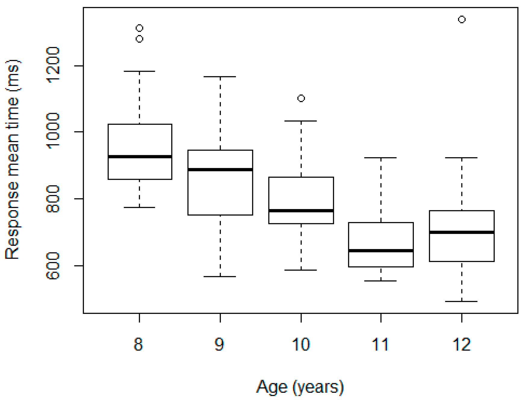
Figure 2 and
Figure 3. We can see that there are only three and four outliers in each case. These cases will be discussed later in detail.
In contrast, the Kruskal-Wallis test revealed statistically significant differences by age (
p-value of 5.27 × 10
−10). Specifically, there were differences for ages between 8 and 9 years, 9 and 10 years, and 10 and 11 years, but not between 11 and 12 years, according to the Wilcoxon test. We repeated the test after eliminating the outlier in the 12-year-old group and the result did not vary. These results are consistent with the findings on how reaction times evolve with age [
38,
61,
62,
63,
64]. A linear model was adjusted taking the logarithm of RT mean as the dependent variable, and age and sex as the fixed-effect factors, obtaining the same results: significant differences across ages 8 and 9 years (10% less RT mean,
p-value = 0.01); 9 and 10 years (8% less,
p-value = 0.05); 10 and 11 years (15% less,
p-value < 0.01); and not between sexes (
p-value for sex 0.82).
4.2. Power-Law Distribution of the NVGs’ Degrees
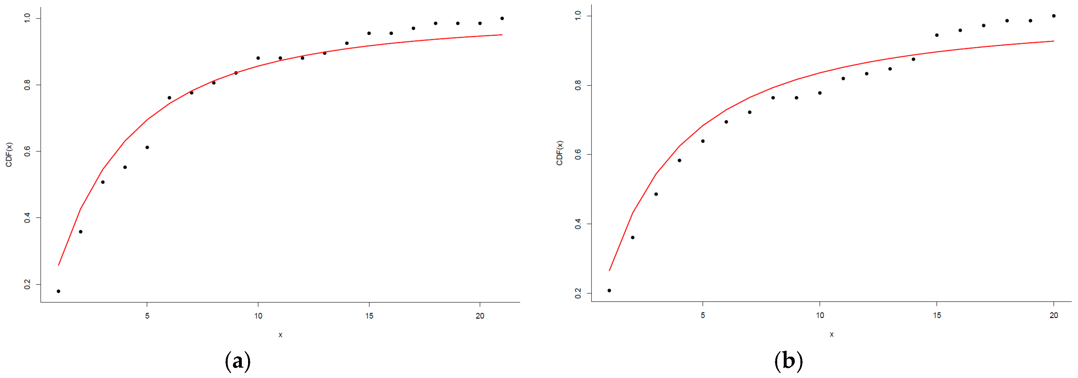
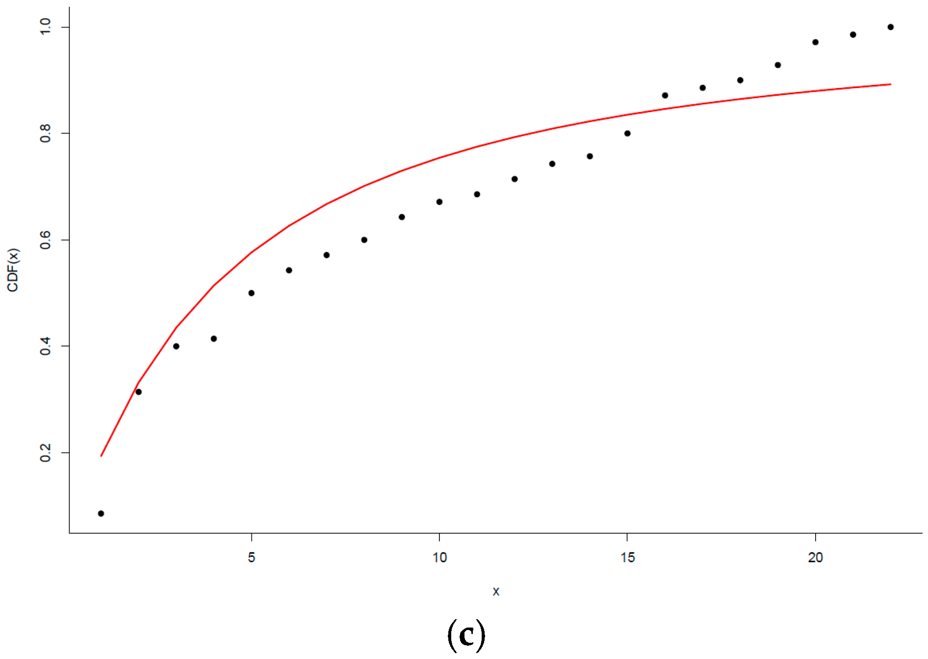
Once we computed the degree distribution of each NVG, we fit each one of these distributions to a power-law, following the procedure described in reference [
41]. For this fit, the relevant values are
α, the exponent of the power-law, and
, the lower bound from which the power-law fit is performed. The use of
is necessary since the fitting of empirical data to a power-law is always performed from this value onwards. We estimate this value
by
, the value that makes it such that for all
, the probability distribution of the empirical data and the best-fit power-law model are as close as possible.
In order to compute the distance between these pairs of distributions, we chose the Kolmogorov-Smirnov (K-S) statistic, which is defined as the maximum distance between the two following cumulative distribution functions (CDFs):
- (a)
, which is the CDF of the empirical data;
- (b)
, which is the CDF for the power-law fit.
In other words, this distance is computed as . Then, is the value of that minimizes .
For computational purposes, the power-law is considered as
where
is the Hurwitz zeta function. Then,
is computed in order to maximize the likelihood function
For specific details, we refer readers to reference [
41].
To explore the goodness-of-fit, we generated a large number of power-law-distributed datasets using as α and
those values obtained from the distribution that best fits the observed data. Each generated dataset was fitted to a power-law distribution, and the K-S statistic was computed with respect to its own model. Then, we counted for the fraction of time that the K-S statistic was larger than the value of the empirical data. The
p-value of the goodness-of-fit was estimated as the fraction of the time that the K-S statistic was larger than that obtained for the observed data. For additional details, we again refer readers to reference [
41].
We point out that the p-values should be interpreted with caution, especially if we are dealing with very few data, as larger p-values do not indicate that the power-law is the most appropriate distribution for our data. The correct interpretation is that it is difficult to discard the power-law when we have few data. In our case, we accepted the power-law distribution for 75% of the students. A summary of the values of the parameter α of the power-law can be found in
Table 3.
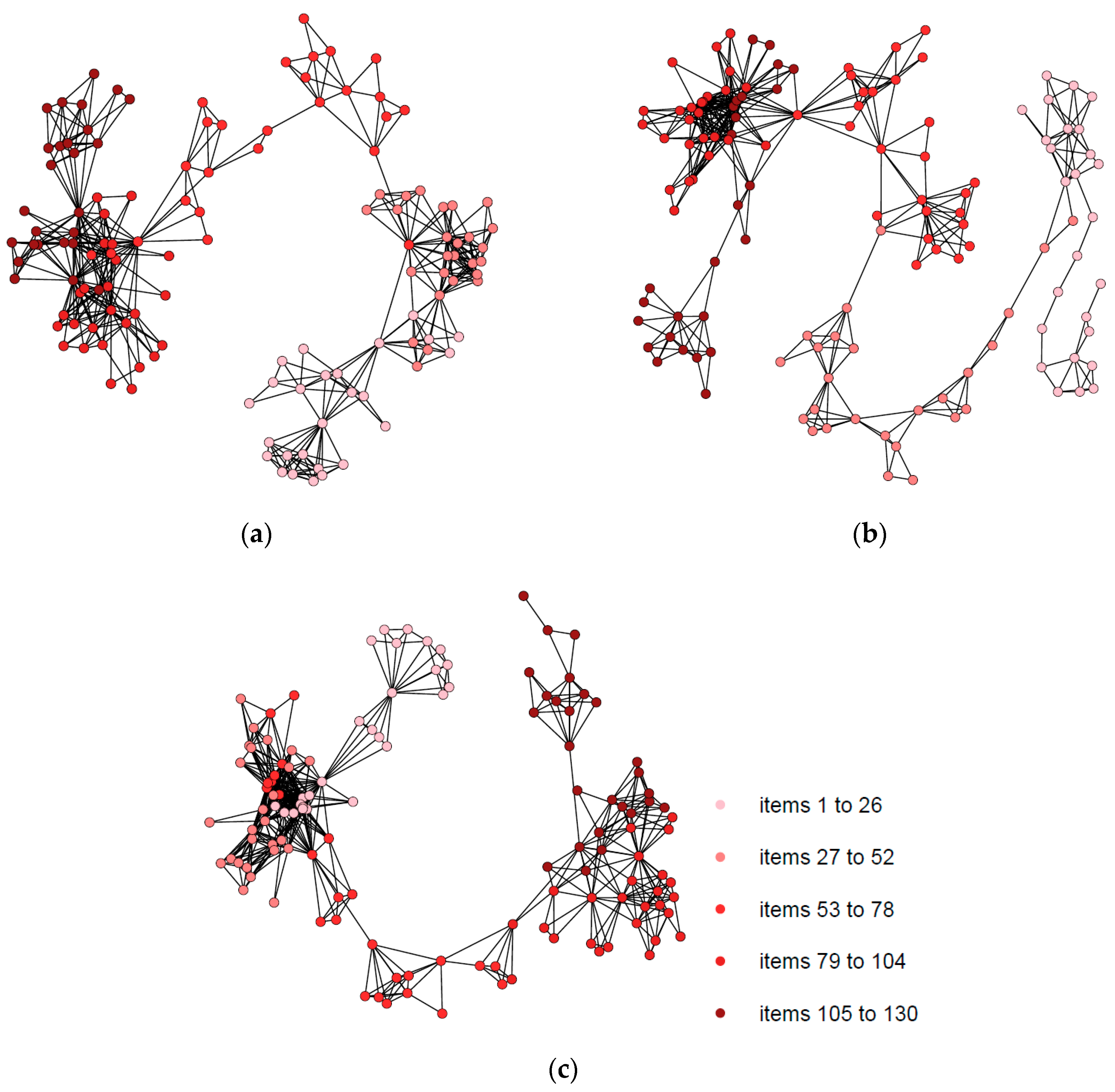
To illustrate the fitting of the degree distribution of NVGs to a power-law distribution, we visualize the NVGs associated with students who did not have omission or commission errors (participants 39, 77, 103) in
Figure 4 and
Figure 5.
In order to study the NVGs’ complexity, we analyzed the Shannon entropy of the NVGs’ degree distributions. Here, it is defined as the expected value of the information content of the variable, that is, the probability that a node
of an NVG has degree
. This was initially considered in this setting by Lacasa et al. [
65]. More precisely, it is defined as
, where
is the number of nodes of each graph, and
is the probability that the node
has degree
. The entropy results are summarized in
Table 4.
There is no association between the Shannon entropy of the degree distribution and the RT means (Spearman correlation of −0.03). In contrast, there is a strong association between the NVGs’ mean degree and the Shannon entropy (Spearman correlation of 0.991).
It is worth mentioning that when analyzing the NVGs’ mean degree, we did not find any statistically significant differences either by sex (
p-value = 0.748 for the Wilcoxon test) or by age (
p-value of 0.8022 for the Kruskal-Wallis test). The results are presented in
Figure 6 and
Figure 7.
Moreover, a linear model including age, sex, and their interaction as predictors and the logarithm of the NVG’s mean degree as response variable was adjusted to corroborate this affirmation. The obtained p-values were 0.530, 0.591, and 0.618 for age, sex, and their interaction, respectively.
4.3. Comparison Between the Power-Law and the Ex-Gaussian Distribution Parameters
Because of the importance of ex-Gaussian distributions in RT analyses, we studied whether there is a relation between NVG complexity and the three parameters that characterize an ex-Gaussian distribution. These parameters represent the mean of the quick responses (
), the standard deviation of the quick responses (
), and the variability of the slow responses (
). It should be noted that there is a strong association between the RT mean and
(Spearman correlation of 0.846) and between the RT mean and
(Spearman correlation of 0.720). There is also a weaker link between the RT mean and
(Spearman correlation of 0.575). The ex-Gaussian parameters for the fitting of the RT frequency distribution were calculated by maximum likelihood as indicated in reference [
32]. A summary of the results is presented in
Table 5.
The α parameter from the power-law fit and the μ and σ parameters are negatively, not statistically significantly correlated, with Spearman correlation coefficients of −0.062 and −0.042, respectively. However, there was a stronger positive association, although not statistically significant, between α and the τ parameter (0.079).
Returning to the aforementioned cases, the results of students 39, 77, and 103 are representative for what is expected of an RT distribution, since their RTs’ frequencies follow ex-Gaussian distributions in each case (see
Figure 8). Despite these participants not committing errors in their answers, they did not need the longest times to respond. Participants 77 and 103 were faster than participant 39 but were older (i.e., 11 years old versus 8 years old).
All parameters, , , , and were positively correlated with the RT mean with correlation coefficients 0.017, 0.768, 0.571, and 0.811, respectively, when response times equal to 2500 ms were not taken into account. However, no association was found when comparing the RT mean with α (Spearman correlation coefficient of 0.017). A linear model was fitted to assess those results obtaining no significant association between the RT mean and α (p-value = 0.140) and between the RT mean and σ (p-value = 0.055).
We found non-remarkable Spearman correlations of the NVG mean degree with (−0.196), (−0.026), (−0.072), and (−0.02). On the other hand, as expected, negative Spearman correlations were also detected between the Shannon entropy and all fitting parameters: (−0.185), (−0.041), (−0.074), and (−0.021).
Finally, three different generalized linear models were adjusted to study the association between , , , and and the number of errors of omission, errors of commission, and hits.
On the one hand, we obtained a significant association between τ and the number of errors of omission. The number of errors of omission increases as long as increases (when increases by 1 unit, omission errors increase 0.7%).
On the other hand, the number of commission errors decreases while μ increases (when μ increases by 1 unit, commission errors decrease 0.2%) and increases while and increase (when σ increases by 1 unit, commission errors increase 0.6%, and when increases by 1 unit, these errors increase 0.3%). These effects remain after adjusting for age and sex. No other significant results were obtained for the other parameters. Finally, the number of hits increases while increases (0.2% more for every increment of by 1 unit), however, the number of hits decreases as and increase (0.5% less when increases by 1 unit, and 0.4% less when increases by 1 unit). All the described effects remain after adjusting the respective models for age and sex.


