Article

LPI Radar Waveform Recognition Based on Deep Convolutional Neural Network Transfer Learning

1
College of Information and Telecommunication, Harbin Engineering University, Harbin 150001, China
2
Key Laboratory of Information System Engineering, The 28th Research Institute of China Electronics Technology Group Corporation, Nanjing 210014, China
*
Author to whom correspondence should be addressed.
Symmetry 2019, 11(4), 540; https://doi.org/10.3390/sym11040540
Submission received: 26 March 2019 / Revised: 9 April 2019 / Accepted: 9 April 2019 / Published: 15 April 2019

Abstract

:
Low Probability of Intercept (LPI) radar waveform recognition is not only an important branch of the electronic reconnaissance field, but also an important means to obtain non-cooperative radar information. To solve the problems of LPI radar waveform recognition rate, difficult feature extraction and large number of samples needed, an automatic classification and recognition system based on Choi-Williams distribution (CWD) and depth convolution neural network migration learning is proposed in this paper. First, the system performs CWD time-frequency transform on the LPI radar waveform to obtain a 2-D time-frequency image. Then the system preprocesses the original time-frequency image. In addition, then the system sends the pre-processed image to the pre-training model (Inception-v3 or ResNet-152) of the deep convolution network for feature extraction. Finally, the extracted features are sent to a Support Vector Machine (SVM) classifier to realize offline training and online recognition of radar waveforms. The simulation results show that the overall recognition rate of the eight LPI radar signals (LFM, BPSK, Costas, Frank, and T1–T4) of the ResNet-152-SVM system reaches 97.8%, and the overall recognition rate of the Inception-v3-SVM system reaches 96.2% when the SNR is −2 dB.

1. Introduction

Low Probability of Intercept (LPI) radar has the characteristics of high resolution, low probability of intercept, time width bandwidth product, and strong anti-jamming ability, which makes it difficult to detect the traditional non-cooperative intercept receiver. Therefore, LPI radar significantly improves the survival ability of the battlefield. It is one of the most effective anti-reconnaissance and anti-jamming technologies. Therefore, how to identify LPI radar signal waveform effectively becomes the focus of non-cooperative radar signal processing research [1,2,3].
The key of LPI radar waveform recognition is to select effective signal features and recognition algorithm. In the 1990s, in [4,5], A.K. Nandi proposed the waveform recognition method of temporal instantaneous and statistical feature extraction. The correct identification success rate of PSK (Phase Shift Keying), FSK (Frequency Shift Keying) and other waveforms is over 90% at SNR of 10 dB. However, it cannot be effectively identified for multiphase code modulation (such as P1 code). In [6,7], Barbarossa adopted Wigner-Ville Distribution (WVD) and Pseudo-Wigner Distribution (PWD) to recognize frequency-modulated signals including LFM and various FM. However, the reference did not study and discuss phase-modulated signals. In [8], Lunden proposed the radar waveform recognition method based on CWD and WVD, and completed the identification of 8 radar waveforms (LFM, BPSK, Costas, Frank code, P1–P4 code). The overall correct classification rate achieves 98% at SNR of 6 dB. However, in a complex noise environment, the accuracy of the recognition success rate is caused by the inaccurate estimation of the carrier frequency and the sub-pulse width by the algorithm. In [9], the method of extracting radar signal waveform features based on CWD time-frequency transform and image processing is proposed combined with ENN neural network classification and recognition. The recognition rate of radar waveforms (LFM, BPSK, Costas, Frank code, P1–P4 code) is 94.7% under the condition of SNR −2 dB. However, these methods do not make full use of other features of the image. Feature extraction not only requires manual design, but also requires many training samples. Seung-Hyun et al. proposed sample averaging techniques and Convolutional Neural Networks (CNNs) for radar waveform recognition [10]. The overall recognition rate of 12 radar waveforms (BPSK, LFM, Costas, Frank, P1–P4, T1–T4) reaches 93.58% at a SNR of −6 dB. However, the large number of samples is required. In addition, the intermediate processing is cumbersome. In [11], time-frequency images (TFIs) and CNNs are used to identify radar waveforms. When analyzing two-dimensional TFIs, a naive approach for dimensionality reduction and denoising is proposed. The simulation results show that the TFI-CNN method has good performance. However, the pre-processing process is cumbersome and complicated, which is a waste of time and poor real-time performance. Therefore, how to extract the effective features of the radar waveform automatically and quickly in the case of small samples and identify more types of LPI radar waveforms under low SNR conditions is a challenging problem.
To reduce the number of training samples, the idea of transfer learning [12,13] was proposed. In [14], Yang used the AlexNet and GoogLeNet model transfer learning methods to pre-grade gliomas. Experiments showed that the performance of the traditional manual extraction features was significantly improved. Michał Byra et al. used the pre-trained Inception-ResNet-v2 deep CNN on the ImageNet dataset to extract high-level features of the liver b-super image sequence [15]. After feature extraction, the support vector machine algorithm was used to contain fatty liver image classification. The experimental results show that the method can effectively diagnose fatty liver content. In [16], the author proposed a technique for automatic classification of abnormal magnetic resonance imaging of brain tumors based on ResNet transfer learning. The classification accuracy of the 613 magnetic resonance images with 5-fold cross-validation reached 100%. In [17], the author proposed the use of deep CNN transfer learning and data augmentation techniques to achieve high-precision classification of coral texture. Experimental results show that the classification performance of this method is significantly better than that of ordinary CNN classification. However, according to recent reports, the idea of transfer learning has not yet been applied to the field of radar waveform recognition.
In summary, the LPI radar waveform recognition based on deep convolution network transfer learning is proposed, which would solve the problems of difficult extraction of traditional CNN LPI radar waveform features, large training samples, complicated time-frequency image pre-processing and low recognition rate of various waveforms under low SNR. The method uses ImageNet trained pre-training models (interception-v3 and ResNet-152) to automatically extract waveform features. This method not only improves the recognition accuracy, but also reduces the number of training samples. The system is mainly composed of three parts: LPI radar waveform CWD time-frequency analysis module, time-frequency image pre-processing module, CNN model migration, and classification module. Firstly, the detected LPI radar waveform is subjected to CWD time-frequency transform. The 1-D time signal is converted into a 2-D time-frequency image. Then the time-frequency image is pre-processed. The purpose is to convert the image into an input image required by the model. The pre-processed images are sent to the CNN recognition model (Inception-v3-SVM or ResNet-152-SVM) for offline training and online classification identification.
The paper is organized as follows. Section 2 is the overall structure of the system. Section 3 introduces signal model and CWD time-frequency analysis. Section 4 designs two CNN migration learning and feature extraction models. Section 5 discusses and analyzes the simulation results after creating the simulation experiments. Finally, Section 6 draws the conclusions.

2. System Overview

In this section, we describe the recognition scheme in detail as shown in Figure 1, the system is mainly composed of two parts: feature extraction and recognition.
The feature extraction part includes three subclasses of CWD time-frequency analysis, time-frequency image pre-processing, and CNN image feature extraction. First, the LPI radar waveform is subjected to CWD time-frequency transform processing to obtain different 2-D time and frequency images. In the time-frequency image, we do not pay attention to the time and frequency values, but on the graphical features of the time-frequency image. Then the image size is adjusted by bi-cubic interpolation algorithm to achieve the resolution of CNN network design. The processed images are sent to the CNN pre-training model for feature extraction.
After the feature extraction is completed, the feature vector is input to the SVM classifier [18] for offline training. After the training is completed, Then the radar signal waveform is input into the system for online identification. The identified signal waveforms include 8 waveforms of LFM, Costas, BPSK, Frank, T1, T2, T3, and T4. The following sections describe the various parts of the system.

3. Signal Model and CWD Time-Frequency Analysis

3.1. Signal Model

We assume that the channel interference is Gaussian white noise, and the SNR is defined as SNR = 10 log 10 ( σ s 2 ) / ( σ ϵ 2 ) [19], where σ s 2 and σ ϵ 2 are the variances of signal and the noise, respectively. Therefore, the signal model is:
y ( n T ) = s ( n T ) + m ( n T ) = A e j ϕ ( n T ) + m ( n T ) ,
where, n is integer. T is sampling interval. s ( n T ) is the complex of detected signal. m ( n T ) is the n-th sampled complex Gaussian white noise. Usually we assume A = 1 . ϕ is the instantaneous phase. Hilbert transform is used to process the detected signal from real signal to complex signal [20].

3.2. Choi-Williams Distribution

The Choi-Williams distribution (CWD) is a kind of time-frequency distribution of Cohen type [21]. By introducing a kernel function, the cross terms generated by multiple signals are suppressed. Therefore, CWD has the characteristics of high resolution and inconspicuous cross terms. The CWD is expressed as follows:
C x ( t , f ) = A x ( η , τ ) Φ ( η , τ ) e j 2 Π ( η t τ f ) d η d τ ,
where:
A x ( η , τ ) = + x ( t , + η / 2 ) x * ( t η / 2 ) e j 2 Π t η d t ,
where f and t are the axes of frequency and time, respectively. Φ ( η , τ ) is a two-dimensional low-pass filter to balance cross terms and resolution. The kernel function is formulated as follows:
Φ ( η , τ ) = e α ( η τ ) 2 ,
α is the controllable factor. The cross terms will be more obvious with the increase of α . In this paper, α = 1 is applied.

3.3. Comparison of Different Signal CWD Time-Frequency Images

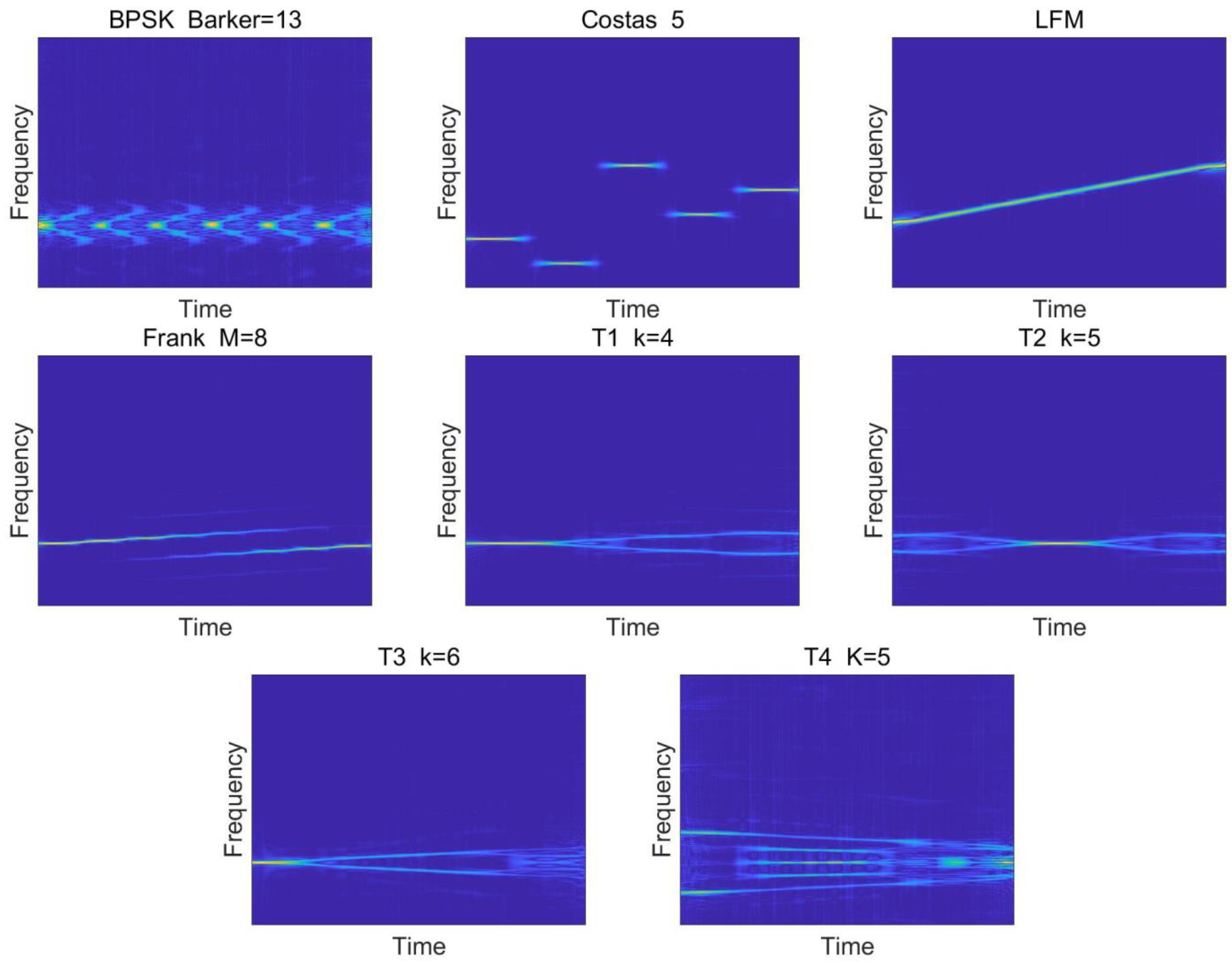
The time-frequency image is obtained as shown in Figure 2 after CWD transformation of 8 LPI radar signals under the condition of SNR = 10 dB. Due to the reduction of interference caused by cross terms, the CWD TFIs of the 8 types of signals accurately reflect the signal modulation period and bandwidth, which provide the basis for subsequent feature extraction. Different modulation patterns of time-frequency signals not only reflect the inherent characteristics of signal modulation, but also open up new ideas and methods for signal waveform detection.

4. CNN Model-Based Transfer Learning and Feature Extraction

The Convolutional Neural Network (CNN) is a common deep learning network architecture inspired by the biological natural visual cognition mechanism. In 1959, Hubel & Wiesel [22] discovered the information processing of the visual system, and the visible cortex was hierarchical. In recent years, the depth and width of CNNs is increasingly influenced by the ILSVRC (ImageNet Large Scale Visual Recognition Challenge) competition in reference [23]. In addition, increasingly complex features can be extracted. In this section, we introduce two typical CNN networks, Inception-v3, and ResNet. Then, we propose the Inception-v3-SVM and ResNet-152-SVM radar waveform recognition models.

4.1. Inception-v3

GoogLeNet [24] is the 2014 ILSVRC champion model with a top-5 error rate of 6.7%. GoogLeNet has made a more effective attempt at network architecture (unlike vgg, which inherits some of the frameworks of GoogLeNet and AlexNet). The model innovatively proposes Inception mechanism. Although there are 22 layers, the parameters are only 1/12 of AlexNet.
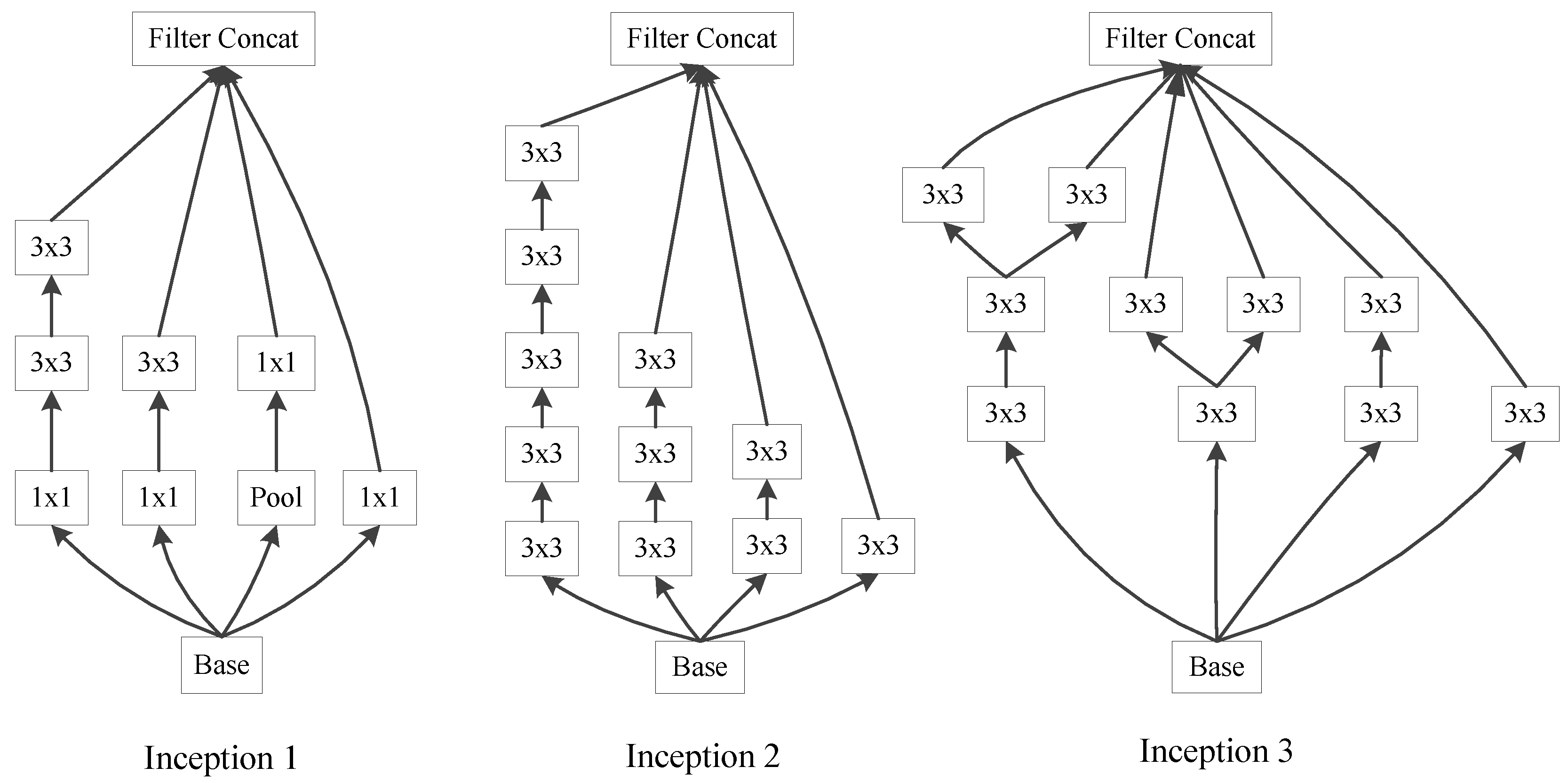
Inception-v3 is one of the GoogLeNet family. Its most important feature is decomposition [25]. The 7 × 7 convolution is dissolved as a 1 × 7 and 7 × 1 convolution. The 3 × 3 convolution is also decomposed into the convolution of 1 × 3 and 3 × 1 , which speeds up the calculation. The solution of one convolution into two convolutions is a further increase in network depth, increasing the nonlinearity of the network. Inception-v3 optimizes the structure of Inception module. The basic Inception-v3 module is shown in Figure 3. In total, Inception-v3 has a total of 42 layers.

4.2. ResNet

ResNet (Residual Neural Network) [26] was proposed by Kaiming He and four other Chinese of Microsoft Research Institute. The 152-layer neural network was successfully trained and won the championship in ILSVRC2015 by using ResNet Unit. The error rate on top5 is 3.57%. The parameter quantity is lower than VGGNet. The effect is very outstanding.
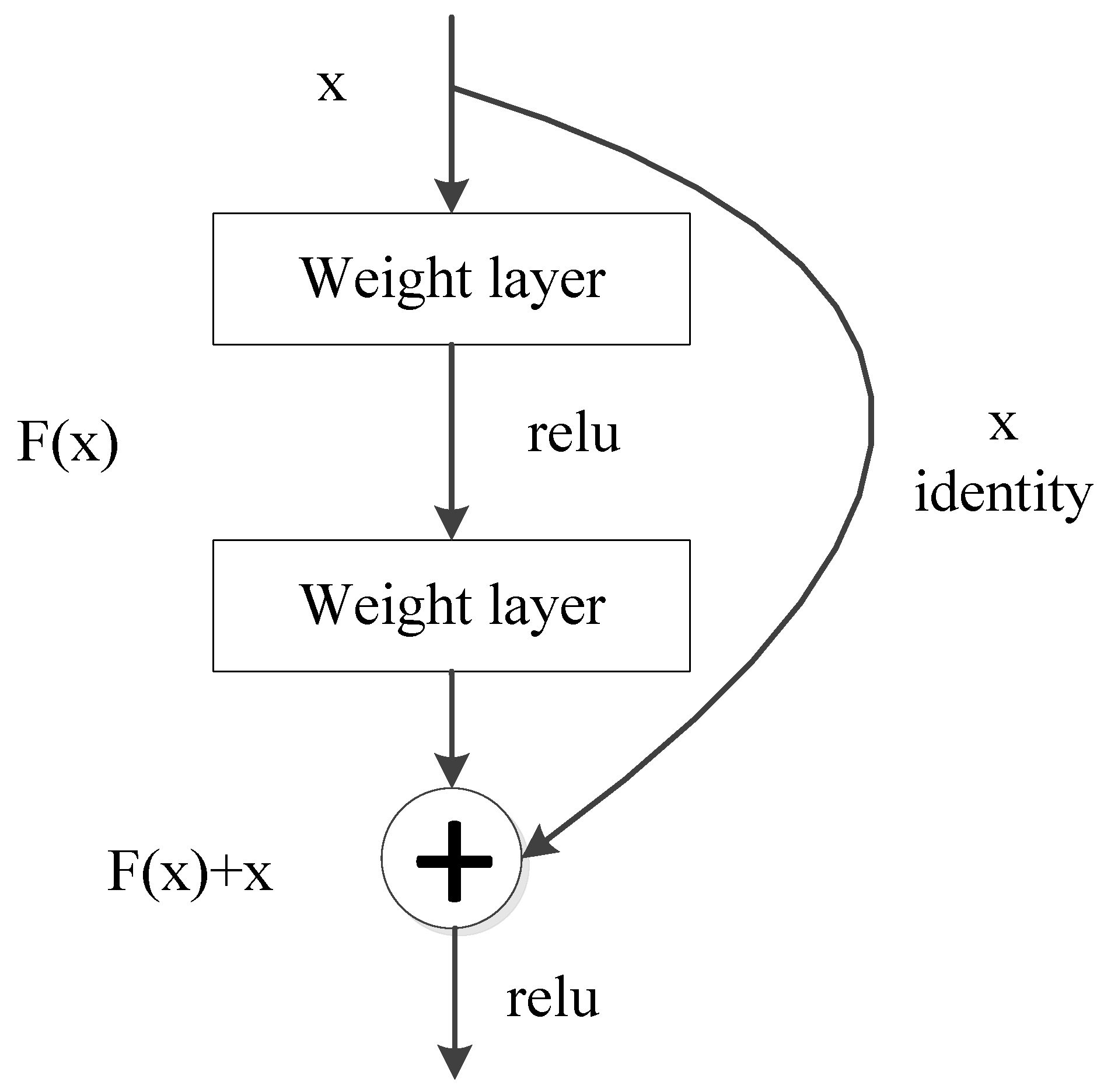
The main idea of ResNet is to add a direct connection channel to the network, which is the idea of the Highway Network. The previous network structure was a nonlinear transformation of the performance input, while the Highway Network allowed a certain percentage of the output of the previous network layer to be retained. The idea of ResNet is very similar to that of Highway Network, allowing raw input information to be passed directly to subsequent layers, as shown in Figure 4.
ResNet has different network layers, the more commonly used are 50-layer, 101-layer, 152-layer. They are all implemented by stacking the residual modules described above. The network configuration of ResNet with different layers is shown in Table 1 below.

4.3. Inception-v3-SVM and ResNet-152-SVM Recognition Model

The CNN model requires a large amount of sample data training to have good generalization ability. However, collecting many samples is time consuming and expensive, so this paper uses the idea of transfer learning to identify less sample radar waveforms.
Transfer Learning [27] is a new machine learning method that uses existing knowledge to solve different but related domain problems. This method relaxes two basic assumptions in traditional machine learning: (1) Samples for learning and new test samples should satisfy the conditions of independent and identical distribution; (2) There must be enough samples to get a good model. Transfer existing knowledge is used to solve the problem that only a small amount of labeled sample data is available even no learning in the target domain [28]. Transfer learning enables the transfer of models from big data to small data for personalized transfer. There are four implementation methods for transfer learning, including: Instance-based Transfer Learning, Feature-based Transfer Learning, Model-based Transfer Learning, and Relational Transfer Learning.
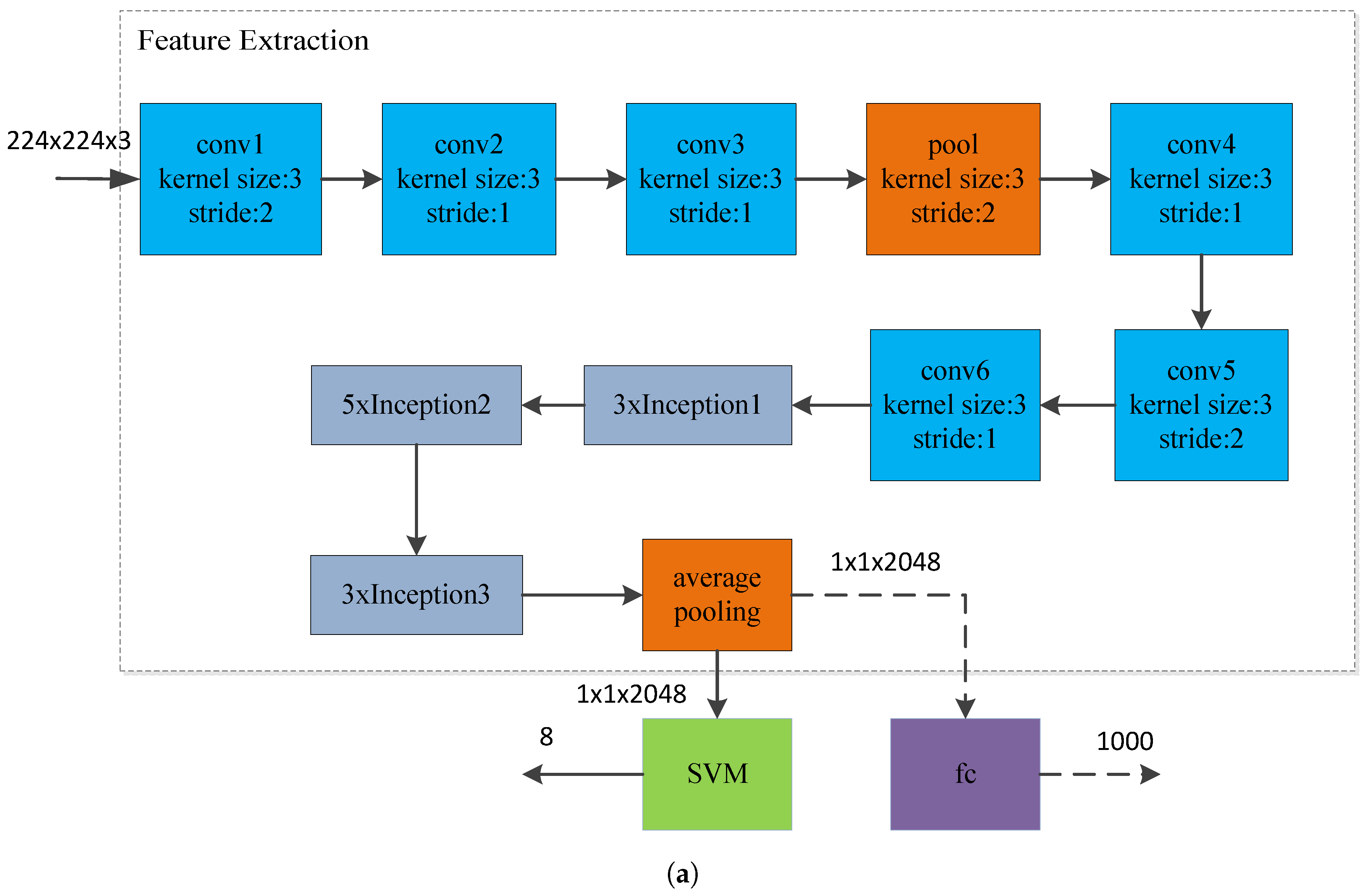
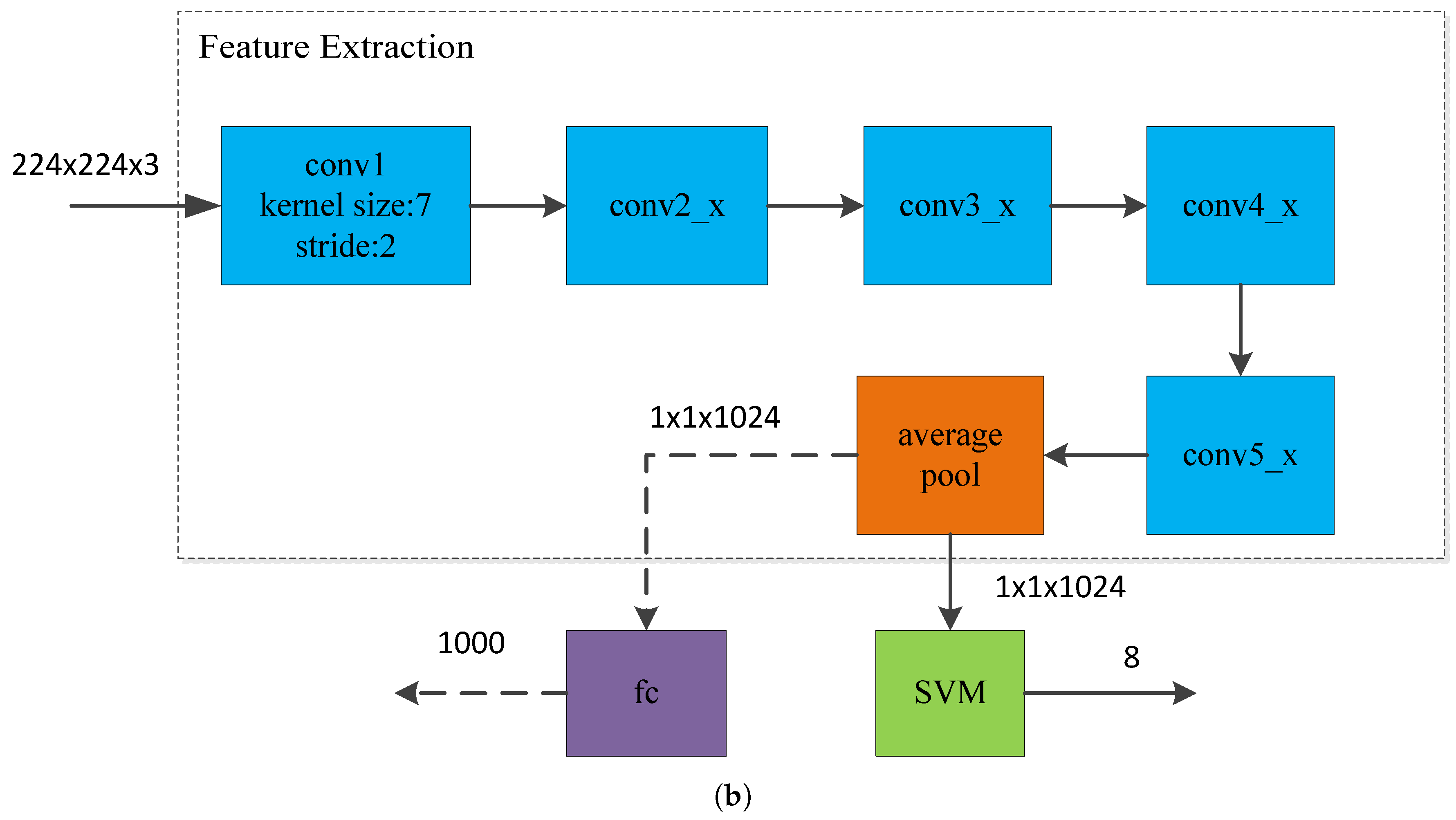
In this paper, transfer learning uses the method of model transfer. Inception-v3 and ResNet-152, the pre-training model of ImageNet, a large natural image data set, are used. Because the paper identifies 8 types of radar waveforms, the probability is that the fully connected layer output in the last layer of the pre-training model is 1000. Category is not applicable in the paper. Therefore, the last layer of the pre-training model is removed. The remaining network structure is treated as a feature extractor. In the pre-training model, different convolution and pooling operations before all average pooling are used to extract features from different dimensions of TFIs. Finally, after all the average pooling, the feature information of different dimensions of the time-frequency image is merged. Therefore, we take the 1 × 1 × 1024 -dimensional vector of all the average pooled output of the original network as the extracted feature. Because the features we extracted are in high-dimensional space, they have the characteristics of nonlinear and small data sets, and the SVM classifier has the characteristics of high precision, good generalization ability, and good robustness in small data sets and nonlinear feature classification. Therefore, our final offline training and online identification use SVM classifier. The specific implementation process is shown in Figure 5.
In the Inception-v3-SVM model of Figure 5a, the structure of Inception1, Inception2, and Inception3 is the basic structure in Inception-v3, as shown in Figure 3 above. In the ResNet-152-SVM model of Figure 5b, conv2_x, conv3_x, conv4_x, and conv5_x are basic convolution operations of the residual network, and the specific structure is shown in Table 1. As shown in Figure 5, the CNN model migration process, the pre-processed time-frequency image ( 224 × 224 × 3 ) is first sent to the pre-training model. The 1 × 1 × 1024 dimension eigenvector is output after passing through the bottleneck layer (the general name of the network before the full connection layer). Finally, the eigenvectors are sent to the SVM classifier to quickly classify the eight radar signal waveforms. Please note that the parameters of the bottleneck layer network of the fixed pre-training model are unchanged during feature extraction. The experimental simulation is shown in the next section.

5. Simulation Experiment and Result Analysis

In this section, we will verify the experimental simulation of the proposed recognition model. The first part of this section gives the simulation parameters of the low intercept probability radar, the second part verifies the validity of the pre-training model extraction feature, the third part verifies the recognition success rate of the proposed model, and the last part verifies the robustness of the proposed system. The details are as follows.

5.1. Sample Creation

It is necessary to generate training data to complete feature extraction and classifier training before the system performs classification and recognition. The sample data generated in this section is used for training and recognition. All the generated data are simulated in the MATLAB 2016a.The detailed parameters of the radar waveform are set as shown in Table 2. U ( · ) is used to denote the normalized frequency to make the list concise. For example, if we assume a certain frequency f 0 = 1000 HZ, and the sampling frequency f s = 8000 HZ, the normalized frequency is expressed as f 0 = U ( f 0 / f s ) = U ( 1 / 8 ) . We set different parameters for different signals. The number of Barker codes used for BPSK signal modulation is randomly selected between 7, 11, and 13. The center frequency ranges from U ( 1 / 8 ) to U ( 1 / 4 ) . The cycles per phase code cpp and code periods number are range of [ 1 , 5 ] and [ 100 , 300 ] respectively. For LFM signals, the signal length is between 500–1024, the initial frequency is set between U ( 1 / 16 ) and U ( 1 / 8 ) , and the bandwidth Δ f is also set at U ( 1 / 16 ) to U ( 1 / 8 ) . The frequency hopping number is set to 3–6 for Costas signal. The frequency hopping fundamental frequency ( f min ) is set between U ( 1 / 24 ) and U ( 1 / 20 ) . For example, when a frequency hopping signal is generated, the frequency hopping frequency is 4. Next, a random non-repetitive sequence is generated, and the difference triangle is satisfied, such as { 3 , 2 , 1 , 4 } . At this time, the frequency of frequency hopping is { 3 f min , 2 f min , f min , 4 f min } . For the Frank signal, the center frequency is a random value between U ( 1 / 16 ) and U ( 1 / 8 ) . cpp is 1 to 5. The samples per frequency steps M is also a random integer with the interval [ 4 , 8 ] . For the multi-time code T1–T4 signal, the number of basic waveform segments is set within the interval [ 4 , 6 ] . In addition, the length of each cycle is normalized within [ 0.07 , 0.1 ] . The signal-to-noise ratio interval is −6 dB to 8 dB, and the step size is 2 dB. Each type of signal produces 100 sets of data for each SNR condition, 80% for training and 20% for testing.

5.2. Feasibility Experiment

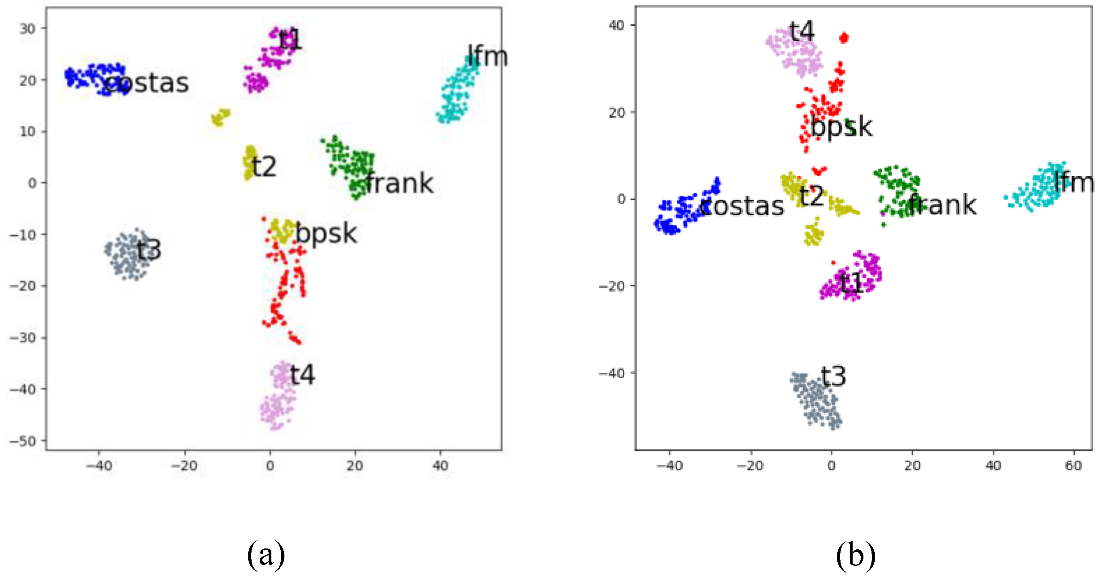
This section of the experiment mainly verifies the feasibility and effectiveness of the CNN pre-training model extraction features. The 100 samples of the 8 types of radar signal waveforms are used under the condition of SNR = 8 dB. The time-frequency image pre-processed by the signal waveform is sent to the pre-training model. In addition, all the averaged pooled feature vectors are extracted. Then the extracted feature vector is reduced by the TSNE algorithm. The result is shown in Figure 6.
It can be seen from Figure 6 that the characteristics of each type of signal are significantly different, which is convenient for classification training and recognition. Therefore, it is feasible to use the migration learning method to extract features.

5.3. Identification Success Rate Experiment

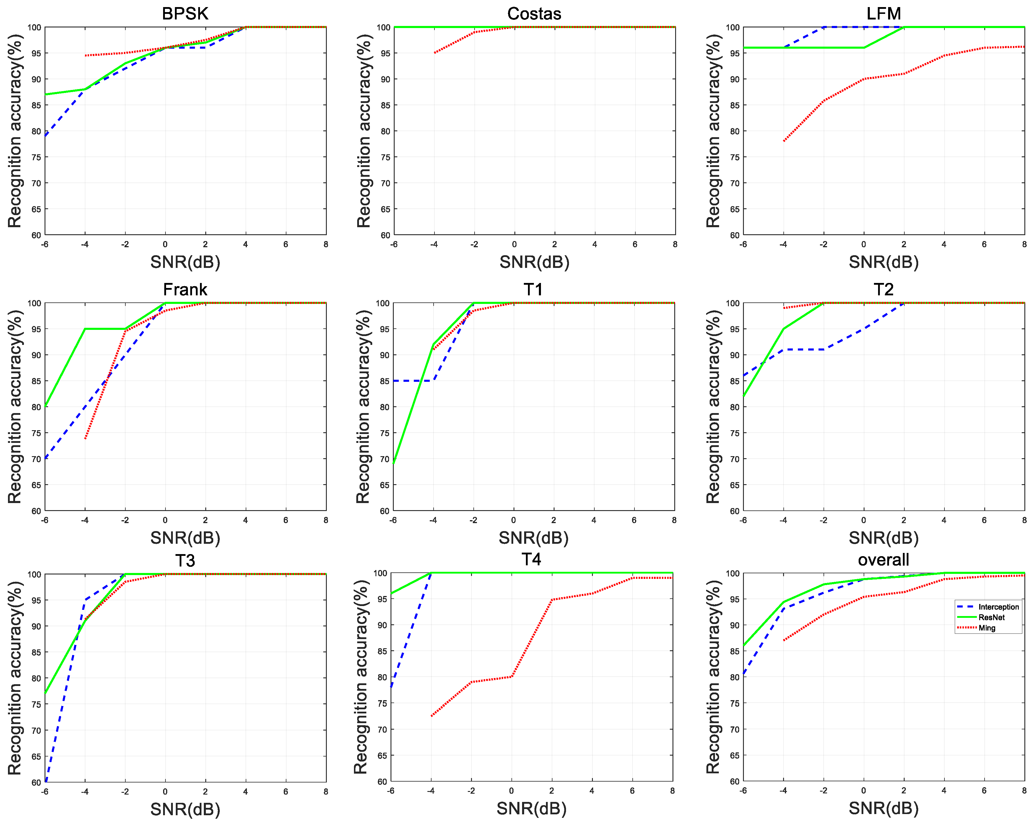
This section of the experiment mainly verifies the relationship between the recognition success rate and the signal-to-noise ratio. 80% of the sample was used for offline training and the remaining 20% was used for testing. The signal-to-noise ratio of the signal increases from −6 dB to 8 dB, and the length is 2 dB. This experiment will be compared with the experiment of Ming [19], because the signal waveform recognized by his proposed system is the same as the waveform identified in this section. It is highly comparable, and his proposed system is one of the outstanding representatives of radar waveform recognition systems. The experimental results are shown in Figure 7.
As shown in Figure 7, the two recognition methods proposed in this section have a recognition success rate of 95% for most radar waveforms with a SNR greater than 0 dB. When the signal-to-noise ratio is greater than 4 dB, the recognition success rate of 8 radar waveforms exceeds 99%. The method has a significant recognition effect on Costas and T4. At lower SNR, both have higher classification success rates. The two methods in this section greatly improve the recognition success rate of LFM, Costas and T4 compared with the reference [19]. In addition, the overall recognition success rate of the two methods in this section is 90% when the SNR is −4 dB. The above is a big improvement over the [19]. The methods proposed in this paper is of great significance to have a good recognition effect under low SNR conditions considering that the radar signal waveform is usually transmitted in a complex environment with low SNR.
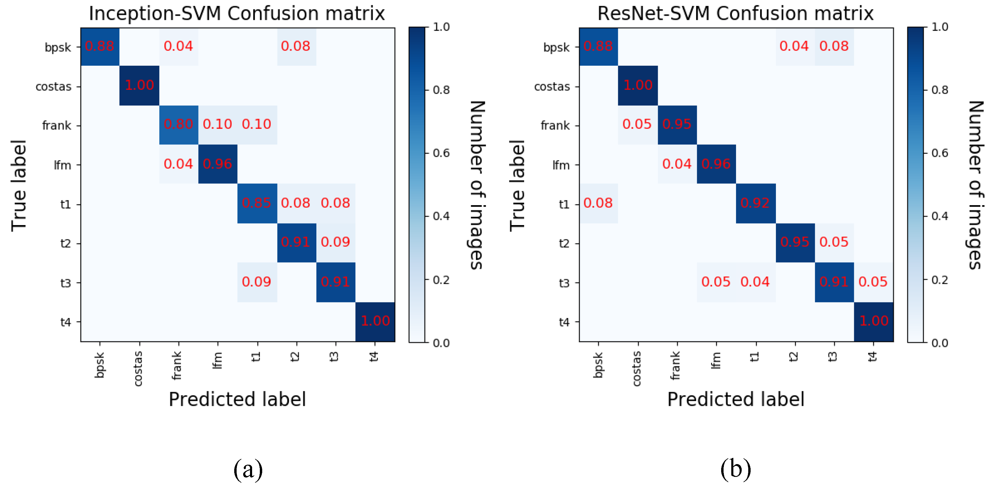
Figure 8 shows the hybrid recognition results of eight radar waveforms with a SNR of −4 dB. At this time, the overall average recognition rate of the ResNet-152-SVM signal is 94.4%, and the overall average recognition rate of the Inception-v3-SVM signal is 92%. In the low SNR condition, the signals with similar TFIs are easily confused. Taking the BPSK signal as an example, 88% of the ResNet-152-SVM identification system is correctly identified as BPSK, 4% is misidentified as T2, and 8% is misidentified as T3 signal.

5.4. Robustness Experiment

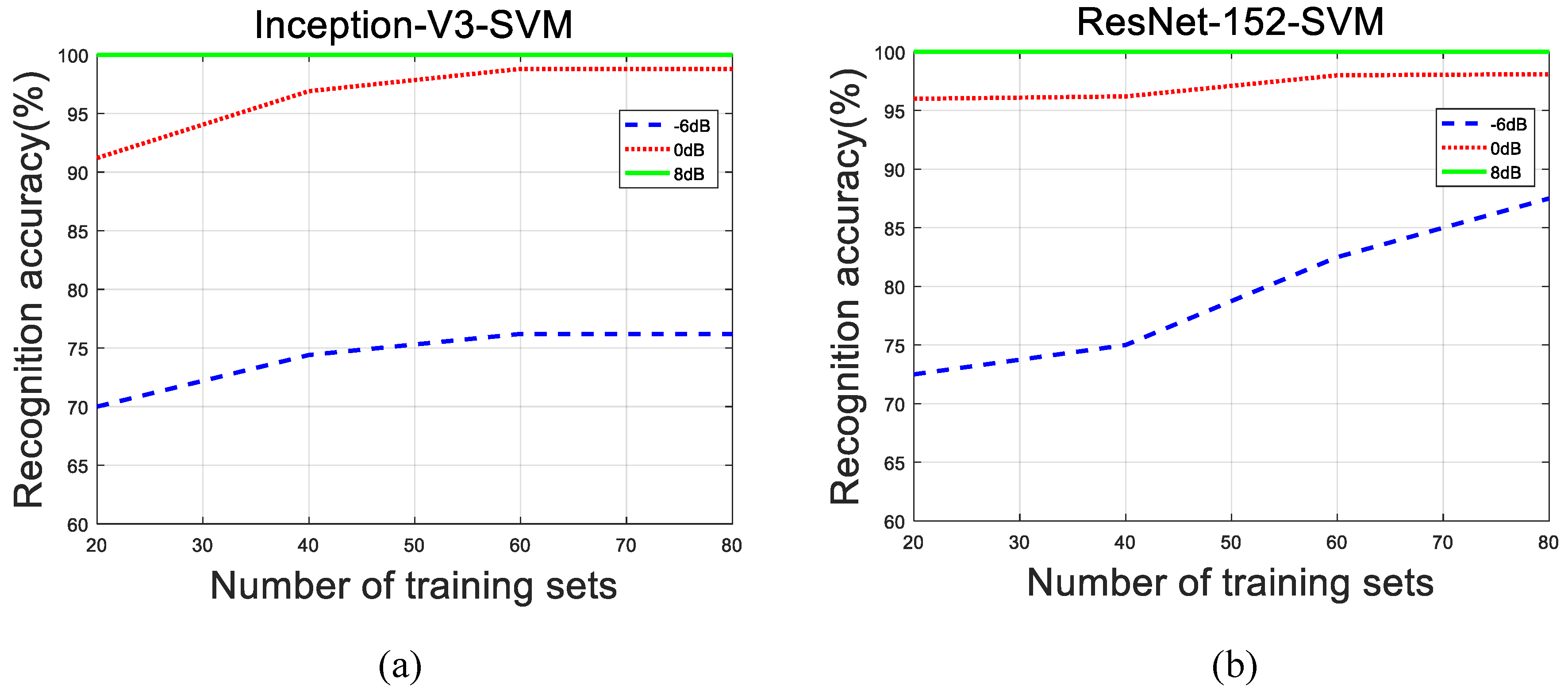
The robustness test is to verify the reliability of the identification method under small sample conditions. For radar waveforms, it is impossible to build a large and complete experimental database like other classification databases. Therefore, the system must have a good correct recognition rate under ultra-small sample conditions. In this experiment, each SNR is 20 signals for testing. The training samples increased from 20 to 80. In addition, the length was 20. Experiments were repeated with −6 dB, 0 dB and 8 dB signal samples, respectively. The experimental results are shown in Figure 9.
As shown in Figure 9, as the training data increases, the overall recognition accuracy of the radar waveform is gradually increased under the three SNR ratios. Under the condition of low SNR, the size of the training set has a great influence on the recognition accuracy. When the SNR = 8 dB, the Inception-v3-SVM is basically stable in 40 sets of sample recognition success rate, and the recognition rate is about 75%. ResNet-152-SVM has a stable recognition success rate curve of 20 groups of training samples at a signal-to-noise ratio of SNR = 0 dB. And its recognition rate is up to 95%. The above shows that the system still has excellent classification performance under the condition of few training samples, which is of great significance for the recognition of radar waveforms.

5.5. Experiment with Computation

Computational complexity issue is an important indicator to measure the performance of classification system. We reproduce Ming method [19], and compare it with this paper in the same conditions. All eight kinds of waveforms are tested under three different SNRs: 6 dB, 0 dB and 8 dB, and each test repeats 10 times on average. The testing environment and testing results are demonstrated as Table 3 and Table 4, respectively.
As shown in Table 4, the Inception-v3-SVM spends about 43 s, the ResNet-152-SVM about 142 s and Mings about 55 s, respectively. In each waveform, there is the trace of reduction in time, when SNR is increasing. Due to the deep layer of ResNet-152 network, the feature extraction process takes a long time, but the classification accuracy is higher. The Inception-v3 network has few layers, fast feature extraction speed, and low complexity. However, the classification accuracy is slightly lower than that of the ResNet-152-SVM under low SNR conditions. In [19], due to the complexity of the pre-processing process, the use of multi-layer perceptron for classification and the back-propagation training mechanism, the training time complexity is high. Under the condition of sufficient time, we use ResNet-152-SVM to classify. Under the condition of high real-time requirements, we use Inception-v3-SVM for classification and recognition.

6. Conclusions

Two LPI radar waveform recognition systems, Inception-v3-SVM and ResNet-152-SVM, are proposed based on the deep CNN and transfer learning ideas. Inception-v3 extracts time-frequency image features from the network width, while ResNet-152 extracts time-frequency image features from the network depth. Both systems can identify 8 LPI radar waveforms (LFM, Costas, BPSK, Frank, and T1–T4) under low SNR conditions, and the system can achieve higher recognition accuracy under the condition that the number of training samples is small. The experimental results show that when the training samples are 80 and the SNR is −2 dB, the recognition rate of ResNet-152-SVM system is as high as 97.8%, and the recognition rate of Inception-v3-SVM system is 96.2%. According to the radar waveform classification, the radiation source can be effectively detected, tracked, and located. It has important application value for wireless communication and radar countermeasure systems.
However, the proposed joint algorithm increases the computational complexity to a certain extent. Therefore, how to use the optimization algorithm [29,30] to optimize the joint algorithm, improve the recognition rate, and reduce the running time is the focus of our future work.

Author Contributions

Q.G. and X.Y. conceived of and designed the experiments. X.Y. performed the experiments. G.R. and X.Y. analyzed the data. X.Y. wrote the paper.

Funding

This work is supported by the Central University Basic Research Business Expenses Special Fund Project (No.HEUCFG201832), the National Key Research and Development Program of China (No.2016YFC0101700), the Heilongjiang Province Applied Technology Research and Development Program National Project Provincial Fund (No.GX16A007), State Key Laboratory Open Fund (No.702SKL201720).

Acknowledgments

The authors would like to thank the editors and the reviewers for their comments on a draft of this article.

Conflicts of Interest

The authors declare no conflict of interest.

Abbreviations

The following abbreviations are used in this manuscript:
LPILow probability of intercept
CWDChoi-Williams distribution
SVMSupport Vector Machine
PSKPhase Shift Keying
FSKFrequency Shift Keying
WVDWigner-Ville Distribution
PWDPseudo-Wigner Distribution
ENNElman neural network
TFITime-frequency images
CNNConvolutional neural network
ILSVRCImageNet Large Scale Visual Recognition Challenge
ReLURectified Linear Unit

References

  1. Tao, C.; Lizhi, L.; Xiangsong, H. LPI Radar Waveform Recognition Based on Multi-Branch MWC Compressed Sampling Receiver. IEEE Access 2018, 6, 30342–30354. [Google Scholar]
  2. Ming, Z.; Ming, D.; Lipeng, G.; Lutao, L. Neural Networks for Radar Waveform Recognition. Symmetry Basel 2017, 9, 75. [Google Scholar] [CrossRef]
  3. Kishore, T.R.; Rao, K.D. Automatic Intrapulse Modulation Classification of Advanced LPI Radar Waveforms. IEEE Trans. Aerosp. Electron. Syst. 2017, 53, 901–914. [Google Scholar] [CrossRef]
  4. Nandi, A.K.; Azzouz, E.E. Algorithms for automatic modulation recognition of communication signals. IEEE Trans. Commun. 1998, 46, 431–436. [Google Scholar] [CrossRef]
  5. Nandi, A.K.; Azzouz, E.E. Automatic analogue modulation recognition. Signal Process. 1995, 46, 211–222. [Google Scholar] [CrossRef]
  6. Barbarossa, S. Analysis of multicomponent LFM signals by a combined Wigner-Hough transform. IEEE Trans. Signal Process. 1995, 43, 1511–1515. [Google Scholar] [CrossRef]
  7. Barbarossa, S.; Lemoine, O. Analysis of nonlinear FM signals by pattern recognition of their time-frequency representation. IEEE Signal Process. Lett. 1996, 3, 112–115. [Google Scholar] [CrossRef]
  8. Lunden, J.; Koivunen, V. Automatic radar waveform recognition. IEEE J. Sel. Top. Signal Process. 2007, 1, 124–136. [Google Scholar] [CrossRef]
  9. Ming, Z.; Lutao, L.; Ming, D. LPI radar waveform recognition based on time-frequency distribution. Sensors 2016, 16, 1682–1706. [Google Scholar]
  10. Kong, S.H. Automatic LPI Radar Wave form Recognition Using CNN. IEEE Access. 2018, 6, 4207–4219. [Google Scholar] [CrossRef]
  11. Chao, W.; Jian, W.; Xudong, Z. Automatic Radar Waveform Recognition Based on Time-Frequency Analysis and Convolutional Neural Network. In Proceedings of the IEEE International Conference on Acoustics, Speech, and Signal Processing (ICASSP), New Orleans, LA, USA, 5–9 March 2017; pp. 2437–2441. [Google Scholar]
  12. Pan, S.J.; Yang, Q. A Survey on Transfer Learning. Knowl. Data Eng. IEEE Trans. 2010, 22, 1345–1359. [Google Scholar] [CrossRef] [Green Version]
  13. Weiss, K.; Khoshgoftaar, T.M.; Dingding, W. A survey of transfer learning. J. Big Data 2016, 3, 9. [Google Scholar] [CrossRef]
  14. Yang, Y.; Lifeng, Y.; Xin, Z.; Yu, H.; Nan, H.Y.; Hu, Y.C.; Hu, B.; Yan, S.L.; Zhang, J.; Cheng, D.L.; et al. Glioma Grading on Conventional MR Images: A Deep Learning Study with Transfer Learning. Front. Neurosci. 2018, 22, 12. [Google Scholar] [CrossRef] [PubMed]
  15. Byra, M.; Styczynski, G.; Szmigielski, C.; Kalinowski, P.; Michalowski, L.; Paluszkiewicz, R.; Ziarkiewicz-Wroblewska, B.; Zieniewicz, K.; Sobieraj, P.; Nowicki, A. Transfer learning with deep convolutional neural network for liver steatosis assessment in ultrasound images. Int. J. Comput. Assist. Radiol. Surg. 2018, 13, 1895–1903. [Google Scholar] [CrossRef]
  16. Talo, M. Application of deep transfer learning for automated brain abnormality classification using MR images. Int. J. Comput. Assist. Radiol. Surg. 2019, 54, 176–188. [Google Scholar] [CrossRef]
  17. Gomez-Rios, A. Towards highly accurate coral texture images classification using deep convolutional neural networks and data augmentation. Exp. Syst. Appl. 2019, 118, 315–328. [Google Scholar] [CrossRef]
  18. Mert, C.; Busemelis, O.; Turgay, I. Image Classification of Aerial Images Using CNN-SVM. In Proceedings of the Innovations in Intelligent Systems and Applications Conference (ASYU), Adana, Turkey, 4–6 October 2018; pp. 89–94. [Google Scholar]
  19. Ming, Z. Convolutional Neural Networks for Automatic Cognitive Radio Waveform Recognition. IEEE Access. 2017, 5, 11074–11082. [Google Scholar]
  20. Xu, B.; Sun, L.; Xu, L.; Xu, G. Improvement of the Hilbert method via ESPRIT for detecting rotor fault in induction motors at low slip. IEEE Trans. Energy Convers. 2013, 28, 225–233. [Google Scholar] [CrossRef]
  21. Liu, Y.; Xiao, P.; Wu, H.; Xiao, W. LPI radar signal detection based on radial integration of Choi-Williams time-frequency image. J. Syst. Eng. Electron. 2015, 26, 973–981. [Google Scholar] [CrossRef]
  22. LeCun, Y.; Bottou, L.; Bengio, Y.; Haffner, P. Gradient-based learning applied to document recognition. Proc. IEEE 1998, 86, 2278–2324. [Google Scholar] [CrossRef] [Green Version]
  23. Russakovsky, O.; Deng, J.; Su, H.; Krause, J.; Satheesh, S. Imagenet large scale visual recognition challenge. Int. J. Comput. Vis. 2015, 115, 211–252. [Google Scholar] [CrossRef]
  24. Szegedy, C.; Wei, L.; Yangqing, J. Going Deeper with Convolutions. In Proceedings of the 2015 IEEE Conference on Computer Vision and Pattern Recognition, Boston, MA, USA, 7–12 June 2015; pp. 1–9. [Google Scholar]
  25. Szegedy, C.; Vanhoucke, V.; Ioffe, S.; Shlens, J.; Wojna, Z. Rethinking the inception architecture for computer vision. In Proceedings of the IEEE conference on computer vision and pattern recognition (CVPR), Seattle, WA, USA, 27–30 June 2016; pp. 2818–2826. [Google Scholar]
  26. Jinyou, Z.; Jiyang, D.; Jiaqi, W.; Jin, Y. Multiobjective Recognition of Unmanned Aerial Vehicle Based on Deep Residual Network. Cartogr. J. 2019, 40, 158–164. [Google Scholar]
  27. Anam, A.M.; Rushdi, M.A. Classification of Scaled Texture Patterns with Transfer Learning. Exp. Syst. Appl. 2018, 120, 448–460. [Google Scholar] [CrossRef]
  28. Fuzhen, Z.; Ping, L.; Qing, H. Survey on Transfer Learning Research. J. Softw. 2015, 26, 26–39. [Google Scholar]
  29. Garg, H. A hybrid GSA-GA algorithm for constrained optimization problems. Inf. Sci. 2019, 478, 499–523. [Google Scholar] [CrossRef]
  30. Garg, H. A hybrid PSO-GA algorithm for constrained optimization problems. Appl. Math. Comput. 2016, 274, 292–305. [Google Scholar] [CrossRef]
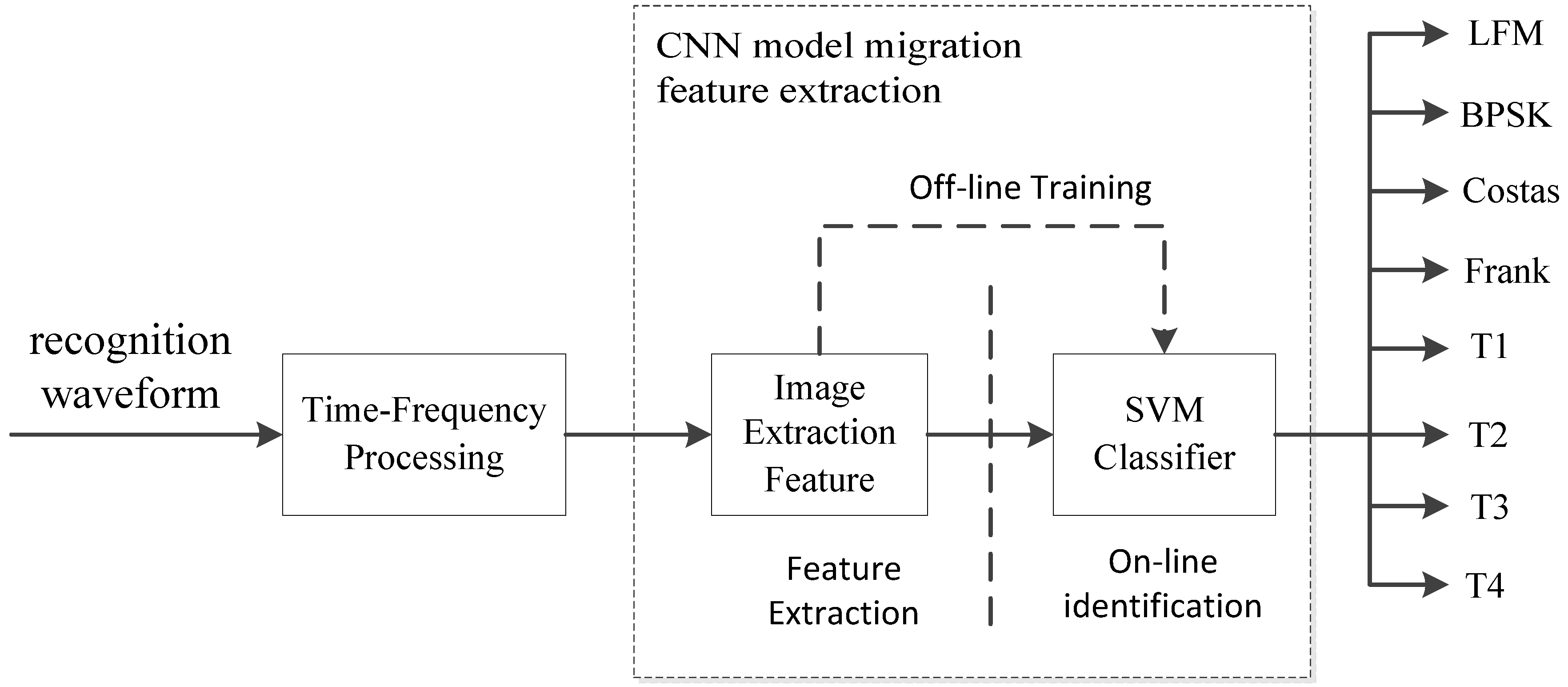
Figure 1. The figure shows the system components.
Symmetry 11 00540 g001
Figure 2. 8 types of LPI radar waveform CWD time-frequency diagram. In this figure, different waveform classes are shown. For BPSK, the number of Barker codes set 13. The Number change in the Costas codes signal set to 5. For the Frank signal, the samples per frequency steps M set 8. For the multi-time code T1–T4 signal, the number of basic waveform segments set 4, 5, 6, 5, respectively. Specific parameter settings are shown in Section 5, Table 2.
Symmetry 11 00540 g002
Figure 3. Basic Inception-v3 structure.
Symmetry 11 00540 g003
Figure 4. ResNet’s residual learning module. In this figure, ReLU is a commonly used activation function in neural networks.
Symmetry 11 00540 g004
Figure 5. CNN model migration process. (a) Inception-v3-SVM; (b) ResNet-152-SVM.
Symmetry 11 00540 g005aSymmetry 11 00540 g005b
Figure 6. 2-D feature map with SNR of 8 dB. (a) ResNet-152 2-D feature map; (b) Inception-v3 2-D feature map.
Symmetry 11 00540 g006
Figure 7. LPI radar waveform recognition rate under different SNR.
Symmetry 11 00540 g007
Figure 8. LPI radar waveform recognition results under −4 dB SNR. (a) ResNet-152-SVM confusion matrix; (b) Inception-v3-SVM confusion matrix.
Symmetry 11 00540 g008
Figure 9. LPI radar waveform recognition accuracy under different training data. (a) ResNet-152-SVM; (b) Inception-v3-SVM.
Symmetry 11 00540 g009
Table 1. Network configuration when ResNet has different layers.
Layer NameOutput Size50-Layer101-Layer152-Layer
conv1 112 × 112 7 × 7 , 64, stride 2
conv2_x 56 × 56 3 × 3 , max pool, stride 2
1 × 1 , 64 3 × 3 , 64 1 × 1 , 256 × 3 1 × 1 , 64 3 × 3 , 64 1 × 1 , 256 × 3 1 × 1 , 64 3 × 3 , 64 1 × 1 , 256 × 3
conv3_x 28 × 28 1 × 1 , 128 3 × 3 , 128 1 × 1 , 512 × 4 1 × 1 , 128 3 × 3 , 128 1 × 1 , 512 × 4 1 × 1 , 128 3 × 3 , 128 1 × 1 , 512 × 4
conv4_x 14 × 14 1 × 1 , 256 3 × 3 , 256 1 × 1 , 1024 × 6 1 × 1 , 256 3 × 3 , 256 1 × 1 , 1024 × 23 1 × 1 , 256 3 × 3 , 256 1 × 1 , 1024 × 36
conv5_x 7 × 7 1 × 1 , 512 3 × 3 , 512 1 × 1 , 2048 × 3 1 × 1 , 512 3 × 3 , 512 1 × 1 , 2048 × 3 1 × 1 , 512 3 × 3 , 512 1 × 1 , 2048 × 3
1 × 1 average pool, 1000-d fc, SoftMax
FLOPs 3.8 × 10 9 7.6 × 10 9 11.3 × 10 9
Table 2. Simulation parameter list [19].
Radar WaveformSimulation ParameterRanges
Sampling frequency f s 1 ( f s = 8000 HZ)
BPSKBarker codes N c { 7 , 11 , 13 }
Carrier frequency f c U ( 1 / 8 , 1 / 4 )
Cycles per phase code c p p [ 1 , 5 ]
Number of code periods n p [ 100 , 300 ]
LFMNumber of samples N [ 500 , 1024 ]
Bandwidth Δ f U ( 1 / 16 , 1 / 8 )
Initial frequency f 0 U ( 1 / 16 , 1 / 8 )
CostasFundamental frequency f min U ( 1 / 24 , 1 / 20 )
Number change N c [ 3 , 6 ]
Number of samples N [ 512 , 1024 ]
FrankCarrier frequency f c U ( 1 / 8 , 1 / 4 )
Cycles per phase code c p p [ 1 , 5 ]
Samples of frequency stem M [ 4 , 8 ]
T1–T4Number of segments k [ 4 , 6 ]
Overall code duration T [ 0.07 , 0.1 ]
Table 3. The testing environment.
ItemModel/Version
CPUi5-8300H (Intel)
GPUNVIDIA GeForce GTX 1050 Ti
Memory16 GB (DDR4@2667 MHZ)
SpyderPython3.5
Table 4. Computational complexity test (Inception-v3-SVM/ ResNet-152-SVM/Ming, Unit: s).
SNR (dB) 6 08
BPSK43.54/141.87/51.3243.43/140.17/51.2043.27/139.25/50.88
Costas43.26/142.35/54.8842.97/141.05/54.0142.62/140.16/53.34
LFM42.79/142.72/55.6042.42/141.09/54.9842.19/139.86/54.78
Frank43.03/145.47/56.3442.76/144.77/56.2942.53/143.28/55.79
T142.68/143.94/58.6342.48/142.86/58.4242.28/141.34/57.68
T243.74/141.31/56.7543.41/139.69/55.8043.14/138.29/55.37
T343.17/140.82/58.8342.89/139.38/58.1142.29/138.04/57.51
T442.98/144.37/54.9042.82/142.97/54.2342.53/141.02/53.90