Single and Multi-Soliton Solutions for a Spectrally Deformed Set of Maxwell-Bloch Equations

Abstract

A specific spectral deformation of the Maxwell-Bloch equations of nonlinear optics is investigated. The Darboux transformation formalism is adapted to this spectrally deformed system to construct its single and multi-soliton solutions. The Effects of spectral deformation on soliton behaviour is studied.

1. Introduction

The spectral deformation technique is a tool of applied mathematics, which enables one to generate many new integrable partial differential equations (pde’s) from a given integrable pde. In its main lines, it can be summarized as follows: Each integrable pde has an associated linear overdetermined system (i.e, a zero curvature representation (ZCR) or a Lax pair) which contains a spectral parameter, $\lambda$. According to the established methods of soliton theory, this parameter must be a constant number. It was first suggested in [1] that under some restrictive assumptions, $\lambda$ can be choosen as a function of the independent parameters of the problem, rather than a constant. The main restriction on $\lambda$ is that it should be the solution of an overdetermined, nonlinear set of pde’s, which was derived in [2]. General solutions for this set of nonlinear pde’s for $\lambda$ are presently not known. However, many different particular solutions can be found by inspection. Each of these particular solutions generates a new, integrable pde from the given integrable pde. These new pde’s are called the “spectral deformations”, or simply “deformations” of the original pde. For some applications of the spectral deformation technique in nonlinear optics, see [3,4,5].

In 1994, the spectral deformation technique was applied to the Maxwell-Bloch (MB) equations of nonlinear optics, which model resonant light–matter interactions [2]. The result was three different deformations, corresponding to three different particular solutions for $\lambda$. Two of these deformations were subsequently solved by employing the dressing and Darboux transformations [2,6]. The third one is not solved yet. Our aim in this paper is to investigate this third equation, which we will call “the deformed Maxwell–Bloch equation” (DMB).

In Section 1, we will summarize the deformation process through which one can generate DMB from MB. Section 2 will develop a Darboux transformation methodology and construct single soliton solutions for DMB. The behaviour of these solitons will be investigated. Section 3 will construct two soliton solutions and investigate soliton collisions.

2. Maxwell-Bloch Equations and Spectral Deformation

Maxwell-Bloch (MB) equations can be expressed as

$$\begin{array}{c}\hfill E_{\eta }=\rho ,\end{array}$$

(1)

$$\begin{array}{c}\hfill N_{\zeta }+\frac{\rho E^{*}+{\rho }^{*}E}{2}=0,\end{array}$$

(2)

$$\begin{array}{c}\hfill {\rho }_{\zeta }+\mathrm{i}\frac{ϵ+{ϵ}^{*}}{2}\rho =NE\end{array}$$

(3)

$$\begin{array}{c}\hfill {ϵ}_{\eta }=0.\end{array}$$

(4)

where $\zeta =t-\frac{x}{c}$, $\eta =\frac{\mathsf{\Omega }}{c}x$. $\mathsf{\Omega }=\frac{4\pi p_0^2{n}_0{\omega }_0}{\hslash }$ is a constant dependent on the physical properties of the system, with $n_0$ being the number of atoms per unit volume, $p_0$ is the polarization and ${\omega }_0$ is the frequency of the electric field. E denotes the complex envelope of the electric field; $\rho$ is the amount of polarization in the resonant medium, and N is the amount of population inversion between the two energy levels. $ϵ$ models frequency shift from the resonance. It is a trivial field as it can be eliminated from the MB equations by rescaling. However, we will not rescale it, as it will become non-trivial when the system is deformed.

It is well-known that MB equations are integrable and possess the following zero curvature representation (ZCR):

$$\begin{array}{c}\hfill {\mathsf{\Psi }}_{\zeta }=J\mathsf{\Psi }\mathsf{\Lambda }+U\mathsf{\Psi },\end{array}$$

(5)

$$\begin{array}{c}\hfill {\mathsf{\Psi }}_{\eta }=V\mathsf{\Psi }{\mathsf{\Lambda }}^{-1},\end{array}$$

(6)

where

$$\begin{array}{c}J=\left[\begin{array}{cc}-\mathrm{i}& 0\\ 0& \mathrm{i}\end{array}\right],\mathsf{\Psi }=\left[\begin{array}{cc}\psi & {\varphi }^{*}\\ \varphi & -{\psi }^{*}\end{array}\right],\mathsf{\Lambda }=\left[\begin{array}{cc}\lambda & 0\\ 0& {\lambda }^{*}\end{array}\right],\\ U=-\frac{1}{2}\left[\begin{array}{cc}\mathrm{i}ϵ& E\\ -E^{*}& -\mathrm{i}{ϵ}^{*}\end{array}\right],V=-\frac{1}{4\mathrm{i}}\left[\begin{array}{cc}N& \rho \\ {\rho }^{*}& -N\end{array}\right],\end{array}$$

(7)

and $\lambda$ is a complex constant. The MB Equations (1)–(4) can be recovered from the ZCR (5) and (6) by equating the mixed derivatives, i.e by ${\mathsf{\Psi }}_{\zeta \eta }={\mathsf{\Psi }}_{\eta \zeta }$, which results in

$$\begin{array}{c}\hfill U_{\eta }=[U,V],\end{array}$$

(8)

$$\begin{array}{c}\hfill V_{\zeta }=[V,J],\end{array}$$

(9)

where [.,.] denotes the commutator. If we substitute the expressions for U, V and J as given in (7) into the above equations, (8) will yield (1), and (4) and (9) will yield (3) and (2). This shows the equivalence of ZCR (5) and (6) to the MB equations.

Note that Equation (3) differs from the original version derived in [2], Equation (9). These two sets of equations are equivalent when the field $ϵ$ is real. However, if the field $ϵ$ is taken to be complex, they cease to be equivalent. Furthermore, the ZCR given in [2] becomes invalid, which indicates that with a complex $ϵ$ field, Equation (9) in [2] loses integrability, while (3) continues to be integrable.

Allowing $ϵ$ to become complex is important, as the Darboux transformations forces it to become complex during the first and subsequent iterations (see Equation (15)). This implies that Darboux transformation cannot be applied directly to Equation (9) in [2] and their ZCR, as these cannot handle a complex $ϵ$ field. Hence, the modifications resulting in Equation (11) is crucial. Furthermore, note that in Equation (11) while $ϵ$ is allowed to be complex, only its real part affects the dynamics of the system.

Spectral deformation of the MB equations is obtained when $\lambda$ is considered not as a constant but as a function of the independent variables $\zeta$ and $\eta$. We are interested in the following specific deformation:

$$\begin{array}{c}\hfill \frac{\partial \lambda }{\partial \zeta }=-b{\lambda }^2,\frac{\partial \lambda }{\partial \eta }=0\Rightarrow \lambda =\frac{k}{bk(\zeta -{\zeta }_0)+1}\end{array}$$

(10)

where b is a real constant and k is a complex integration constant which is called the ‘hidden spectral parameter’ in the spectral deformation literature. Enforcing the consistency conditions ${\mathsf{\Psi }}_{\zeta \eta }={\mathsf{\Psi }}_{\eta \zeta }$ yields

$$\begin{array}{c}\hfill U_{\eta }=[U,V]+bV,\\ \hfill V_{\zeta }=[V,J],\end{array}$$

or, when (7) is substituted,

$$\begin{array}{c}{E}_{\eta }=(1-\mathrm{i}b/2)\rho ,\\ N_{\zeta }+(\rho E^{*}+{\rho }^{*}E)/2=0,\\ {\rho }_{\zeta }+\mathrm{i}\frac{ϵ+{ϵ}^{*}}{2}\rho =NE,\\ {ϵ}_{\eta }=-bN/2.\end{array}$$

(11)

These equations will be called the deformed Maxwell–Bloch equations (DMB) in the rest of this article. The physical meaning of Equation (11) is not clear, but we consider it interesting anyway to study them from a mathematical point of view.

3. Single Soliton Solution for DMB

There are many methods to compute soliton solutions of integrable equations and these methods usually work well with the spectrally deformed versions of the same equations. Recent examples that specifically relate to optical solitons are [7,8,9,10,11], which use a plethora of closely related techniques like Darboux transformations, Dressing transformations or Backlund transformations. This article will use Darboux transformations to construct solitons of DMB.

For the seed solution, choose

$$\begin{array}{ccc}\hfill E=0,& & \rho =0,\hfill \\ \hfill N=N_0,& & ϵ={ϵ}_0-\frac{b{N}_0}{2}\eta ,\hfill \end{array}$$

by inspection, where $N_0$, ${ϵ}_0$ are real constants. Substituting these into (7), and solving for $\mathsf{\Psi }$ in (5)–(6) with $\lambda$ as defined in (10) gives

$$\begin{array}{ccc}\hfill \psi & =& K_{1}exp\left[-\frac{\mathrm{i}}{b}ln(bk(\zeta -{\zeta }_0)+1)-\frac{\mathrm{i}{ϵ}_0}{2}(\zeta -{\zeta }_0)+\frac{\mathrm{i}b{N}_0}{4}(\zeta -{\zeta }_0)\eta +\frac{\mathrm{i}{N}_0}{4k}\eta \right],\hfill \\ \hfill \varphi & =& K_{2}exp\left[\frac{\mathrm{i}}{b}ln(bk(\zeta -{\zeta }_0)+1)+\frac{\mathrm{i}{ϵ}_0}{2}(\zeta -{\zeta }_0)-\frac{\mathrm{i}b{N}_0}{4}(\zeta -{\zeta }_0)\eta -\frac{\mathrm{i}{N}_0}{4k}\eta \right].\hfill \end{array}$$

The Darboux iteration maps a solution $S_0=\{U,V,\mathsf{\Psi }\left(\lambda \right)\}$ of the ZCR (5) and (6) to another solution $S_1=\{\overline{U},\overline{V},\overline{\mathsf{\Psi }}\left(\lambda \right)\}$ of the same ZCR. In practice, it is enough to specify a transformation that maps $\mathsf{\Psi }\left(\lambda \right)$ to $\overline{\mathsf{\Psi }}\left(\lambda \right)$. Two other transformations which map $\{U,V\}$ to $\{\overline{U},\overline{V}\}$ follow as an extension to this transformation.

The following ansatz is proposed for mapping $\mathsf{\Psi }\left(\lambda \right)$ to $\overline{\mathsf{\Psi }}\left(\lambda \right)$:

$$\begin{array}{c}\hfill \overline{\mathsf{\Psi }}\left(\lambda \right)=\mathsf{\Psi }\left(\lambda \right)+Q\mathsf{\Psi }\left(\lambda \right){\mathsf{\Lambda }}^{-1}\end{array}$$

(12)

where $Q(x,t)$ is a $2\times 2$ matrix whose exact form is to be determined. This ansatz differs from the standard one used commonly in Darboux transformation theory, given as

$$\begin{array}{c}\hfill \overline{\mathsf{\Psi }}\left(\lambda \right)=\mathsf{\Psi }\left(\lambda \right)\mathsf{\Lambda }+Q\mathsf{\Psi }\left(\lambda \right).\end{array}$$

which only generates trivial solutions for DMB. By contrast, the newly proposed transformation (12) generates nontrivial solutions. To specify $Q(\zeta ,\eta )$ it is sufficient to fix a zero of $\overline{\mathsf{\Psi }}\left(\lambda \right)$, i.e, choose ${\lambda }_1$ such that $\overline{\mathsf{\Psi }}\left({\lambda }_1\right)=0$ for all $\zeta$ and $\eta$. Here ${\lambda }_1$ denotes $\lambda$ evaluated at a hidden spectral parameter $k=k_1$.

$$\begin{array}{c}\hfill {\lambda }_1=\frac{k_1}{b{k}_1(\zeta -{\zeta }_1)+1}\end{array}$$

(13)

This implies the form of the matrix Q:

$$\begin{array}{c}\hfill Q=-{\mathsf{\Psi }}_1{\mathsf{\Lambda }}_1{\mathsf{\Psi }}_1^{-1}\end{array}$$

and $\overline{\mathsf{\Psi }}\left(\lambda \right)=\mathsf{\Psi }(\lambda ,{\lambda }_1)$

$$\begin{array}{ccc}\hfill \mathsf{\Psi }(\lambda ,{\lambda }_1)& =& \mathsf{\Psi }-{\mathsf{\Psi }}_1{\mathsf{\Lambda }}_1{\mathsf{\Psi }}_1^{-1}\mathsf{\Psi }{\mathsf{\Lambda }}^{-1},\hfill \end{array}$$

(14)

The subscript 1 above (as in ${\mathsf{\Lambda }}_1$ and ${\mathsf{\Psi }}_1$) denotes that k and ${\zeta }_0$ in $\mathsf{\Lambda }$ and $\mathsf{\Psi }$ are fixed at $k=k_1$ and ${\zeta }_0={\zeta }_1$. The next step is to construct the matrices $\overline{U}=U\left({\lambda }_1\right)$ and $\overline{V}=V\left({\lambda }_1\right)$ satisfying

$$\begin{array}{ccc}\hfill \mathsf{\Psi }{(\lambda ,{\lambda }_1)}_{\zeta }& =& J\mathsf{\Psi }(\lambda ,{\lambda }_1)\mathsf{\Lambda }+U\left({\lambda }_1\right)\mathsf{\Psi }(\lambda ,{\lambda }_1)\hfill \\ \hfill \mathsf{\Psi }{(\lambda ,{\lambda }_1)}_{\eta }& =& V\left({\lambda }_1\right)\mathsf{\Psi }(\lambda ,{\lambda }_1){\mathsf{\Lambda }}^{-1}\hfill \end{array}$$

After substituting (14) into the the zero curvature representation above and using (5)–(6) to convert the result into an algebraic equation, we arrive at the final result:

$$\begin{array}{ccc}\hfill U\left({\lambda }_1\right)& =& U+[J,{\mathsf{\Psi }}_1{\mathsf{\Lambda }}_1{\mathsf{\Psi }}_1^{-1}]-b{\mathsf{\Psi }}_1{\mathsf{\Lambda }}_1{\mathsf{\Psi }}_1^{-1},\hfill \\ \hfill V\left({\lambda }_1\right)& =& {\mathsf{\Psi }}_1{\mathsf{\Lambda }}_1{\mathsf{\Psi }}^{-1}V{\mathsf{\Psi }}_1{\mathsf{\Lambda }}_1^{-1}{\mathsf{\Psi }}_1^{-1}.\hfill \end{array}$$

Carrying out the algebra, we find all the fields (which are elements of the matrices $U\left({\lambda }_1\right)$ and $V\left({\lambda }_1\right)$) corresponding to a single-soliton solution:

$$\begin{array}{ccc}E\left({\lambda }_1\right)& =& -4\frac{K_2^{*}}{K_2}\left(1-\frac{ib}{2}\right)\Im \left({\lambda }_1\right)e^{i{a}_1}\mathrm{sech}\left({\beta }_1\right)\hfill \\ \rho \left({\lambda }_1\right)& =& -4\frac{K_2^{*}}{K_2}\frac{\partial }{\partial \eta }\left(\Im \left({\lambda }_1\right)e^{i{a}_1}\mathrm{sech}\left({\beta }_1\right)\right)\hfill \\ N\left({\lambda }_1\right)& =& N_0-4\Im \left({\lambda }_1\right)\frac{\partial }{\partial \eta }tanh\left({\beta }_1\right)\hfill \\ ϵ\left({\lambda }_1\right)& =& 2b\Im \left({\lambda }_1\right)tanh\left({\beta }_1\right)-2b\Re \left({\lambda }_1\right)i+{ϵ}_0-\frac{b{N}_0\eta }{2}\hfill \end{array}$$

(15)

where

$$\begin{array}{ccc}\hfill a_1& =& -\frac{2}{b}|bk(\zeta -{\zeta }_1)+1|-{ϵ}_0(\zeta -{\zeta }_1)+\frac{b{N}_0}{2}(\zeta -{\zeta }_1)\eta +\frac{N_0}{2|k_1{|}^2}\Re \left(k_1\right)\eta ,\hfill \end{array}$$

(16)

$$\begin{array}{ccc}\hfill {\beta }_1& =& -\frac{2}{b}arctan\left(\frac{b(\zeta -{\zeta }_1)\Im \left(k_1\right)}{b(\zeta -{\zeta }_1)\Re \left(k_1\right)+1}\right)+\frac{N_0\Im \left(k_1\right)}{2|k_1{|}^2}\eta +ln\frac{|K_1|}{|K_2|}.\hfill \end{array}$$

(17)

Here $\Im (.)$, $\Re (.)$ denote the real and imaginary parts of a complex number. Note that due to the term $2b\Re \left({\lambda }_1\right)i$ the field $ϵ\left({\lambda }_1\right)$ becomes complex after the application of the Darboux transformation.

Figure 1 plots the electric field of the single-soliton solution vs. $\zeta$ and $\eta$. Contrary to the undeformed MB equation, the soliton of the DMB equation is a transient. It pops out of the background, attains a maximum, and then decays back into the background. This can be seen much better in Figure 2, which indicates that the soliton has a “lifetime”, i.e., it has a significant magnitude only for $-300<\eta <300$. Furthermore, the soliton does not travel at a uniform speed. The soliton stops for some time before it grows or after it decays, which can be observed in Figure 3.

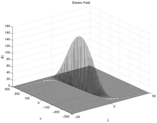
Figure 1. E-field vs. $\zeta$ and $\eta$ for b = 0.015, k = −2 + 0.1i, $N_0$ = −60 and ${ϵ}_0=0$.

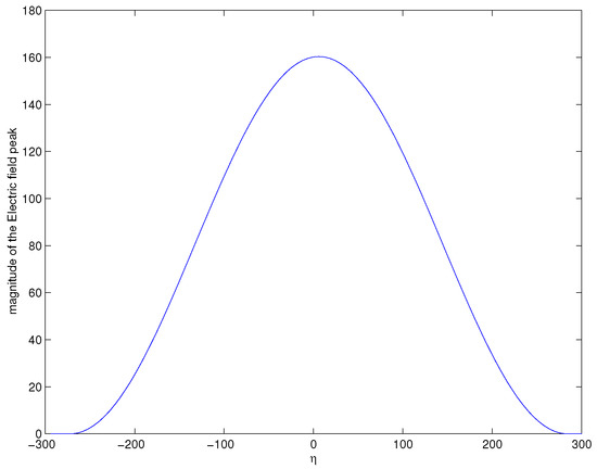
Figure 2. Magnitude of the electric field peak vs. $\eta$. Parameters are the same with Figure 1.

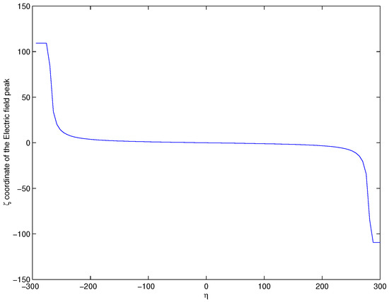
Figure 3. Position of the electric field peak vs. $\eta$. Parameters are the same with Figure 1.

One can also ask the question if the DMB soliton behaves more like the MB soliton as $b\to 0$. Figure 4 and Figure 5 demonstrate that this is the case. There is a region around $\eta =0$ in which the soliton travels with approximately constant amplitude and speed, like the MB soliton. As b becomes smaller, this region gets wider.

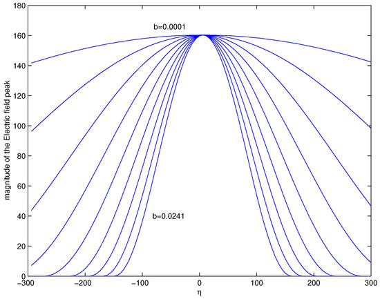
Figure 4. Magnitude of the electric field peak vs. $\eta$ for various values of b, from b = 0.001 to b = 0.0241 with steps $\Delta$b = 0.003. All other parameters are the same with Figure 1.

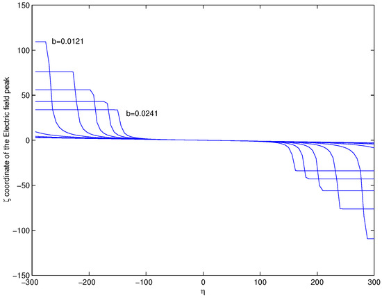
Figure 5. Position of the peak of electric field vs. $\eta$ for various values of b, from b = 0.001 to b = 0.0241 with steps $\Delta$b = 0.003. All other parameters are the same with Figure 1.

4. Two-Soliton Solution

Using $\mathsf{\Psi }(\lambda ,{\lambda }_1)$, $U\left({\lambda }_1\right)$ and $V\left({\lambda }_1\right)$ found above as seed solutions, we can also compute a two-soliton solution, whose E can be given by

$$\begin{array}{ccc}E({\lambda }_2,{\lambda }_1)& =& -4\left(1-\frac{\mathrm{i}b}{2}\right)\hfill \\ & \times & \frac{I_2{e}^{\mathrm{i}{a}_2}\mathrm{sh}\left({\beta }_2\right)+I_1{e}^{\mathrm{i}{a}_1}\mathrm{sh}\left({\beta }_1\right)-\frac{2\mathrm{i}(R_2-R_1)I_1{I}_2}{|{\lambda }_2{|}^2-2R_2{R}_1+{\left|{\lambda }_1\right|}^2}\left(e^{\mathrm{i}{a}_2}\mathrm{th}\left({\beta }_1\right)\mathrm{sh}\left({\beta }_2\right)-e^{\mathrm{i}{a}_1}\mathrm{sh}\left({\beta }_1\right)\mathrm{th}\left({\beta }_2\right)\right)}{1-\frac{I_1{I}_2}{|{\lambda }_2{|}^2-2R_2{R}_1+{\left|{\lambda }_1\right|}^2}\left[2\mathrm{th}\left({\beta }_2\right)\mathrm{th}\left({\beta }_1\right)+\mathrm{sh}\left({\beta }_2\right)\mathrm{sh}\left({\beta }_1\right)(e^{\mathrm{i}(a_2-a_1)}+e^{\mathrm{i}(a_1-a_2)})\right]},\hfill \end{array}$$

where $a_2$, ${\beta }_2$ are defined in the same way with $a_1$, ${\beta }_1$ in Equations (16) and (17) with the substitutions $k_2\to k_1$ and ${\zeta }_2\to {\zeta }_1$. Also, $\mathrm{sh}(.)$, $\mathrm{th}(.)$ denote $\mathrm{sech}(.)$, $tanh(.)$. $R_{1,2}$, $I_{1,2}$ denote $\Re \left({\lambda }_{1,2}\right)$ and $\Im \left({\lambda }_{1,2}\right)$, respectively.

Figure 6 demonstrates two solitons in collision, where $b=0.2$, $k_1=0.1-0.85\mathrm{i}$, $k_2=0.2+0.4\mathrm{i}$ and ${\zeta }_1={\zeta }_2=0$. As in the undeformed case, the faster soliton passes through the smaller one elastically, without losing its shape.

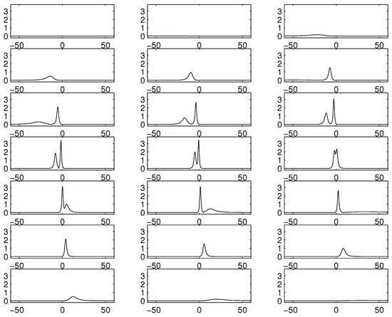
Figure 6. |E|-field for the collison of two solitons between $\eta =-0.56$ and $\eta =0.46$. $-60<\zeta <60$, b = 0.2, $k_1$ = 0.1 − 0.85i, $k_2$ = 0.2 + 0.4i, ${ϵ}_0$ = 0, $N_0$ = −60.

5. Discussion

A Darboux-transformation based methodology to construct the soliton solutions of the DMB equation is proposed. These solitons are shown to behave quite differently compared to the well-known MB solitons, as they have a finite lifetime, constantly changing shape and nonuniform speed. It is also shown that as the deformation parameter b goes to zero, DMB solitons behave more and more like the MB soliton. In all other respects, DMB solitons have the usual soliton behaviour, like elastic collisions.

References

- Belinskii, V.A.; Zakharov, V.E. Integration of Einstein equations by means of inverse scattering problem technique and construction of exact soliton solutions. Sov. Phys. JETP 1978, 48, 985–994. [Google Scholar]
- Burtsev, S.P.; Gabitov, I. Alternative integrable equations of nonlinear optics. Phys. Rev. 1994, 49, 2065–2070. [Google Scholar] [CrossRef]
- Nakkeeran, K. Optical solitons in Ebrium doped fibers with higher order effects and pumping. J. Phys. 2000, 33, 4377–4381. [Google Scholar]
- Porsezian, K. Soliton models in resonant and nonresonant optical fibers. Pramana J. Phys. 2001, 57, 1003–1039. [Google Scholar] [CrossRef]
- Porsezian, K. Optical solitons in some SIT type equations. J. Mod. Opt. 2000, 47, 1635–1644. [Google Scholar] [CrossRef]
- Rybin, A. Application of Darboux transformations to problems with variable spectral parameters. J. Phys. 1991, 24, 5235–5243. [Google Scholar] [CrossRef]
- Gao, J.W.; Huang, Y.H.; Tian, Y.J.; Yong, X. Darboux transformation and nonautonomous solitons for a generalized inhomogeneous hirota equation. Indian J. Phys. 2016, 91, 129–138. [Google Scholar]
- Rajan, S.M.; Arumugam, M. Multi-soliton propagation in a generalized inhomogeneous nonlinear Schrödinger-Maxwell-Bloch system with loss/gain driven by an external potential. J. Math. Phys. 2013, 54, 043514. [Google Scholar] [CrossRef]
- Guo, R.; Tian, B.; Lv, X.; Zhang, H.Q.; Liu, W.J. Darboux Transformation and Soliton Solutions for the Generalized Coupled Variable Coefficient Nonlinear Schrödinger-Maxwell-Bloch System with Symbolic Computation. Indian J. Phys. 2016, 91, 129–138. [Google Scholar] [CrossRef]
- Han, K.H.; Shin, H.J. Nonautonomous integrable nonlinear Schrödinger equations with generalized external potentials. J. Phys. A: Math. Theor. 2009, 42, 335202. [Google Scholar] [CrossRef]
- Perumal, S.; Porsezian, K.; Ramanathan, G. Optical solitons in some deformed MB and NLS–MB equations. Phys. Lett. 2006, 348, 233–243. [Google Scholar]
© 2019 by the author. Licensee MDPI, Basel, Switzerland. This article is an open access article distributed under the terms and conditions of the Creative Commons Attribution (CC BY) license (http://creativecommons.org/licenses/by/4.0/).