Anti-Saturation Control of Uncertain Time-Delay Systems with Actuator Saturation Constraints

Abstract

The problem of anti-saturation control for a class of time-delay systems with actuator saturation is considered in this paper. By introducing appropriate variable substitution, a new delay time-delay systems model with actuator saturation systems is established. Based on the Lyapunov stability theory, the stability condition and the anti-saturation controller design method are obtained by using the linear matrix inequality approach. By introducing the matrix into the Lyapunov function, the proposed conditions are less conservative than the previous results. Finally, a simulation example shows the validity and rationality of the method.

1. Introduction

The saturation phenomenon exists widely in various power systems. If saturation limitation is not considered, the performance of the system will be degraded or even unstable in severe cases. In practical engineering control processes, control input often needs to satisfy certain conditions, and actuator saturation is the most common constraint phenomenon, so research on actuator saturation control has very important practical significance. Since Fuller first proposed a saturation system in the 1960s, actuator saturation control has attracted extensive attention from many scholars [1,2,3]. Hu et al. proposed a convex combination method for discrete linear systems with actuator saturation by utilizing saturation nonlinearity [4]. By introducing auxiliary matrices, the stability conditions are transformed into linear matrix inequalities (LMIs), and the stability conditions of the system and the design method of the controller are obtained. Then, Zhou et al. introduced the design method of a saturated system into a saturated networked control system. For example, the output feedback stabilization of a saturated networked system is studied in reference [5]. Some scholars have studied the time-delay systems with saturation constraints. Reference [6] considers the stabilization of networked control systems affected by actuator saturation and network-induced delays. In reference [7], a distributed model with predictive control is designed for a stochastic polyhedral uncertain system with limited actuator saturation. Recently, the auxiliary time-delay feedback technique has been used to deal with the stabilization of neutral time-delay systems with actuator saturation [8]. Using the saturation technique of nested actuators, Zhou et al. studied the stability analysis and the estimation of the attractive region of discrete linear systems [9]. In reference [10], an improved delay-dependent control method with low conservativeness was proposed for actuator saturated control systems with time-varying delays. In addition, the actuator saturation problem also appears in the networked control system, which is very meaningful and challenging. Based on the finite-time theory, Ma et al. considered the delay-dependent control stability conditions and anti-saturation control problems of discrete singular Markov jump systems. By using the linear matrix inequality method, sufficient conditions for the finite-time boundedness of singular systems have been obtained. By using the method of multiple Lyapunov functions, a new sufficient condition for stochastic finite-time boundedness of the system is obtained [11,12]. In reference [13], by using suitable Lyapunov functions and new criteria of attraction domains, low conservative conditions for stochastic stability of the system were given. It overcomes the difficulty of estimating the attraction region in system analysis and synthesis. Subsequently, Song et al. studied the problem of quantized feedback stabilization for continuous time-delay systems with actuator saturation. By using two different methods, the delay-independent conditions for system stability have been obtained [14]. In reference [15], the influence of network bandwidth on the system performance has been considered. Then, a new network system model is established. A dynamic allocation strategy of bandwidth of networked control systems has been obtained.

However, the above literature mainly focuses on deterministic systems, while the research on saturated time-delay systems with uncertainties is rare. For this reason, based on the previous studies, this paper presents the sufficient conditions for asymptotic stability of a class of uncertain time-delay systems with actuator saturation by using LMIs and Lyapunov stability theory. Then, the design scheme of anti-saturation controllers were obtained by introducing parameter matrices into Lyapunov functions.

2. Preliminaries

Consider the following uncertain time-delay systems with input saturation:

$$\begin{array}{l}\dot{x}(t)=(A+\Delta A(t))x(t)+(A_d+\Delta A_d(t))x(t-d)+(B+\Delta B(t))sat(u(t))\\ x(t)=\varphi (t) t\in [-d,0].\end{array}$$

(1)

where $x(t)\in {\mathrm{R}}^{\mathrm{n}}$ are systems states, $u(t)\in {\mathrm{R}}^{\mathrm{m}}$ are control input, $A,A_d\in {\mathrm{R}}^{\mathrm{n}\times \mathrm{n}}$, $B\in {\mathrm{R}}^{\mathrm{n}\times m}$ are a constant matrix, $\phi (t)={[{\phi }_1(t){\phi }_2(t)\cdots {\phi }_n(t)]}^T\in {\mathrm{R}}^{\mathrm{n}}$ is the given initial state, $d$ is the state delay of the systems. The saturation function $sat(u(t))=[sat(u_1(t)),sat(u_2(t)),\cdots ,sat(u_m(t))]$, where

$$sat(u_i(t))=\{\begin{array}{ll}{\underset{\_}{u}}_i& u_i(t)\le {\underset{\_}{u}}_i<0\\ u_i(t)& {\underset{\_}{u}}_i\le u_i(t)\le {\overline{u}}_i\\ {\overline{u}}_i& 0<{\overline{u}}_i\le u_i(t).\end{array}$$

$\Delta A(t),\Delta A_d(t),\Delta B(t)$ is the system uncertainty with appropriate dimension, satisfying:

$$\Delta A(t)=D_{1}F(t)E_1,\Delta A_d(t)=D_{2}F(t)E_2,\Delta B(t)=D_{3}F(t)E_3].$$

(2)

where the matrix function $F(t)$ satisfying $F^T(t)F(t)\le I$.

The state feedback controller of the systems (1) is designed:

$$u(t)=2Kx(t).$$

(3)

where $K\in {\mathrm{R}}^{m\times n}$ is a undetermined constant matrix. Substitute (2) into the systems (1) to obtain a closed-loop system:

$$\begin{array}{ll}\dot{x}(t)=\overline{A}(t)x(t)+{\overline{A}}_d(t)x(t-d)+& \overline{B}(t)\eta (t)\\ x(t)=\varphi (t)& t\in [-d,0].\end{array}$$

(4)

where

$$\begin{array}{l}\overline{A}(t)=A+BK+\Delta A(t)+\Delta B(t)K\\ {\overline{A}}_d(t)=A_d+\Delta A_d(t)\\ \overline{B}(t)=B+\Delta B(t)\\ \eta (t)=sat(2Kx(t))-Kx(t).\end{array}$$

(5)

and $\eta (t)$ satisfying:

$${\eta }^T(t)\eta (t)\le x^T(t)K^{T}Kx(t).$$

(6)

The purpose of the design is to determine the controller such as (3) so that the closed-loop system (4) is asymptotically stable.

Lemma 1.

For the given constant matrix$Y,D$and$E$with appropriate dimension, where$Y$is symmetric matrix, then$Y+DEF+E^T{F}^T{D}^T<0$for matrix$F$satisfying$F^{T}F\le I$, if and only if there is a constant$\epsilon >0$, such that:

$$Y+\epsilon D{D}^T+{\epsilon }^{-1}{E}^{T}E<0.$$

Lemma 2

([8]). For a given n-order symmetric matrix $S=\left[\begin{array}{cc}{S}_{11}& S_{12}\\ S_{21}& S_{22}\end{array}\right]$, where $S_{11}$ is r-order matrix, then the following three conditions are equivalent:

(1)

$S<0,$

(2)

$S_{11}<0,S_{22}-S_{12}^T{S}_{11}^{-1}{S}_{12}<0,$

(3)

$S_{22}<0,S_{11}-S_{12}{S}_{22}^{-1}{S}_{12}^T<0.$

3. Main Results

Theorem 1.

If there is a constant$\epsilon >0$, symmetrical positive matrix$P,Q\in {\mathrm{R}}^{n\times n}$and matrix$K\in R^{m\times n}$satisfying the matrix inequality:

$$\Theta =\left[\begin{array}{ccc}{\overline{A}}^T(t)P+P\overline{A}(t)+Q+\epsilon K^{T}K& P{\overline{A}}_d(t)& P\overline{B}(t)\\ \ast & -Q& 0\\ \ast & \ast & -\epsilon I\end{array}\right]<0.$$

(7)

Then the closed-loop system (4) is asymptotically stable.

Proof. 

Using the positive definite matrix $P,Q$ to construct the function:

$$V(t)=x^T(t)Px(t)+{\displaystyle {\int }_{t-d}^t{x}^T(s)Qx(s)}ds,$$

$P,Q\in {\mathrm{R}}^{n\times n}$ are undetermined symmetric positive matrices.

With the solution of Equation (3), it is easy to obtain:

$$\begin{array}{ll}\dot{V}(t)=& 2x^T(t)P\dot{x}(t)+x^T(t)Qx(t)-x^T(t-d)Qx(t-d)\\ & =x^T(t)(P\overline{A}(t)+{\overline{A}}^T(t)P)x(t)+2x^T(t)P{\overline{A}}_d(t)x(t-d)+2x^T(t)P\overline{B}(t)\eta (t)\\ & +x^T(t)Qx(t)-x^T(t-d)Qx(t-d)\\ & ={\Phi }^T(t)\left[\begin{array}{ccc}P\overline{A}(t)+{\overline{A}}^T(t)P& P{\overline{A}}_d(t)& P\overline{B}(t)\\ \ast & -Q& 0\\ \ast & \ast & 0\end{array}\right]\Phi (t),\end{array}$$

(8)

where

$$\Phi (t)=\left[\begin{array}{c}x(t)\\ x(t-h)\\ \eta (t)\end{array}\right].$$

From the formula (6), we can obtain:

$$0\le {\Phi }^T(t)\left[\begin{array}{ccc}\epsilon K^{T}K& 0& 0\\ \ast & 0& 0\\ \ast & \ast & -\epsilon I\end{array}\right]\Phi (t),$$

where $\epsilon$ is an arbitrarily small positive number.

Inserting the upper formula into (8) formula and get

$$\dot{V}(t)\le {\Phi }^T(t)\Theta \Phi (t),$$

where

$$\Theta =\left[\begin{array}{ccc}{\overline{A}}^T(t)P+P\overline{A}(t)+Q+\epsilon K^{T}K& P{\overline{A}}_d(t)& P\overline{B}(t)\\ \ast & -Q& 0\\ \ast & \ast & -\epsilon I\end{array}\right].$$

According to Lyapunov stability theory, when condition (7) holds, the closed-loop system (4) is asymptotically stable. ☐

Theorem 2.

If there are constants$\overline{\epsilon }>0,{\epsilon }_1>0,{\epsilon }_2>0,{\epsilon }_3>0$, symmetrical positive matrices$X,\overline{Q}\in {\mathrm{R}}^{n\times n}$and matrix$\overline{K}\in R^{m\times n}$satisfying the matrix inequality:

$$\left[\begin{array}{ccccccc}\Xi & A_{d}X& {\epsilon }^{-1}B& {\overline{K}}^T& X{E}_1^T& X{E}_3^T& X{E}_2^T\\ \ast & -\overline{Q}& 0& 0& 0& 0& 0\\ \ast & \ast & -\overline{\epsilon }I& 0& 0& 0& 0\\ \ast & \ast & \ast & -\overline{\epsilon }I& 0& 0& 0\\ \ast & \ast & \ast & \ast & -{\epsilon }_{1}I& 0& 0\\ \ast & \ast & \ast & \ast & \ast & -{\epsilon }_{3}I& 0\\ \ast & \ast & \ast & \ast & \ast & \ast & -{\epsilon }_{2}I\end{array}\right]<0.$$

(9)

where $\Xi =AX+B\overline{K}+{(AX+B\overline{K})}^T+\overline{Q}+{\epsilon }_1{D}_1{D}_1^T+{\epsilon }_2{D}_2{D}_2^T+{\epsilon }_3{D}_3{D}_3^T$

Then the closed-loop system (4) is asymptotically stable. Closed-loop systems (4) are asymptotically stable by selecting the controller $u(t)=2\overline{K}{X}^{-1}x(t)$.

Proof. 

With the Lemma 1, the inequality (7) is equivalent to:

$$\left[\begin{array}{cccc}{\overline{A}}^T(t)P+P\overline{A}(t)+Q& P{\overline{A}}_d(t)& P\overline{B}(t)& \epsilon K^T\\ \ast & -Q& 0& 0\\ \ast & \ast & -\epsilon I& 0\\ \ast & \ast & \ast & -\epsilon I\end{array}\right]<0.$$

The matrix $diag\{P^{-1},P^{-1},{\epsilon }^{-1}I,{\epsilon }^{-1}I\}$ is multiplied at both sides of the upper formula, we obtain:

$$\left[\begin{array}{cccc}{P}^{-1}{\overline{A}}^T(t)+\overline{A}(t)P^{-1}+P^{-1}Q{P}^{-1}& {\overline{A}}_d(t)P^{-1}& {\epsilon }^{-1}\overline{B}(t)& P^{-1}{K}^T\\ \ast & -P^{-1}Q{P}^{-1}& 0& 0\\ \ast & \ast & -{\epsilon }^{-1}I& 0\\ \ast & \ast & \ast & -{\epsilon }^{-1}I\end{array}\right]<0.$$

Inserting formula (4) into the upper formula:

$$\Sigma +\left[\begin{array}{cccc}\Delta A(t)P^{-1}+\Delta B(t)K{P}^{-1}+{(\Delta A(t)P^{-1}+\Delta B(t)K{P}^{-1})}^T& \Delta A_d(t)P^{-1}& {\epsilon }^{-1}\Delta B(t)& 0\\ \ast & 0& 0& 0\\ \ast & \ast & 0& 0\\ \ast & \ast & \ast & 0\end{array}\right]<0.$$

where

$$\Sigma =\left[\begin{array}{cccc}A{P}^{-1}+BK{P}^{-1}+{(A{P}^{-1}+BK{P}^{-1})}^T+P^{-1}Q{P}^{-1}& A_d{P}^{-1}& {\epsilon }^{-1}B& P^{-1}{K}^T\\ \ast & -P^{-1}Q{P}^{-1}& 0& 0\\ \ast & \ast & -{\epsilon }^{-1}I& 0\\ \ast & \ast & \ast & -{\epsilon }^{-1}I\end{array}\right].$$

Inserting formula (2) into the upper formula:

$$\begin{array}{l}\Sigma +\left[\begin{array}{c}{D}_1\\ 0\\ 0\\ 0\end{array}\right]F(t)\left[\begin{array}{cccc}{E}_1{P}^{-1}& 0& 0& 0\end{array}\right]+{\left[\begin{array}{cccc}{E}_1{P}^{-1}& 0& 0& 0\end{array}\right]}^T{F}^T(t){\left[\begin{array}{c}{D}_1\\ 0\\ 0\\ 0\end{array}\right]}^T\\ \left[\begin{array}{c}{D}_2\\ 0\\ 0\\ 0\end{array}\right]F(t)\left[\begin{array}{cccc}{E}_2{P}^{-1}& 0& 0& 0\end{array}\right]+{\left[\begin{array}{cccc}{E}_2{P}^{-1}& 0& 0& 0\end{array}\right]}^T{F}^T(t){\left[\begin{array}{c}{D}_2\\ 0\\ 0\\ 0\end{array}\right]}^T\end{array}$$

$$\begin{array}{l}\left[\begin{array}{c}{D}_3\\ 0\\ 0\\ 0\end{array}\right]F(t)\left[\begin{array}{cccc}0& 0& {\epsilon }^{-1}{E}_3& 0\end{array}\right]+{\left[\begin{array}{cccc}0& 0& {\epsilon }^{-1}{E}_3& 0\end{array}\right]}^T{F}^T(t){\left[\begin{array}{c}{D}_3\\ 0\\ 0\\ 0\end{array}\right]}^T\\ <0.\end{array}$$

With Lemma 2, if there are constants ${\epsilon }_1>0,{\epsilon }_2>0,{\epsilon }_3>0$ such that the upper formula be equivalent to:

$$\begin{array}{l}\Sigma +{\epsilon }_1\left[\begin{array}{c}{D}_1\\ 0\\ 0\\ 0\end{array}\right]{\left[\begin{array}{c}{D}_1\\ 0\\ 0\\ 0\end{array}\right]}^T+{\epsilon }_1^{-1}{\left[\begin{array}{cccc}{E}_1{P}^{-1}& 0& 0& 0\end{array}\right]}^T\left[\begin{array}{cccc}{E}_1{P}^{-1}& 0& 0& 0\end{array}\right]\\ +{\epsilon }_2\left[\begin{array}{c}{D}_2\\ 0\\ 0\\ 0\end{array}\right]{\left[\begin{array}{c}{D}_2\\ 0\\ 0\\ 0\end{array}\right]}^T+{\epsilon }_2^{-1}{\left[\begin{array}{cccc}{E}_2{P}^{-1}& 0& 0& 0\end{array}\right]}^T\left[\begin{array}{cccc}{E}_2{P}^{-1}& 0& 0& 0\end{array}\right]\\ +{\epsilon }_3\left[\begin{array}{c}{D}_3\\ 0\\ 0\\ 0\end{array}\right]{\left[\begin{array}{c}{D}_3\\ 0\\ 0\\ 0\end{array}\right]}^T+{\epsilon }_3^{-1}{\left[\begin{array}{cccc}0& 0& {\epsilon }^{-1}{E}_3& 0\end{array}\right]}^T\left[\begin{array}{cccc}0& 0& {\epsilon }^{-1}{E}_3& 0\end{array}\right]<0.\end{array}$$

With Lemma 1, we know:

$$\left[\begin{array}{ccccccc}\begin{array}{l}A{P}^{-1}+BK{P}^{-1}\\ +{(A{P}^{-1}+BK{P}^{-1})}^T\\ +P^{-1}Q{P}^{-1}+{\epsilon }_1{D}_1{D}_1^T\\ +{\epsilon }_2{D}_2{D}_2^T+{\epsilon }_3{D}_3{D}_3^T\end{array}& A_d{P}^{-1}& {\epsilon }^{-1}B& P^{-1}{K}^T& P^{-1}{E}_1^T& P^{-1}{E}_3^T& P^{-1}{E}_2^T\\ \ast & -P^{-1}Q{P}^{-1}& 0& 0& 0& 0& 0\\ \ast & \ast & -{\epsilon }^{-1}I& 0& 0& 0& 0\\ \ast & \ast & \ast & -{\epsilon }^{-1}I& 0& 0& 0\\ \ast & \ast & \ast & \ast & -{\epsilon }_{1}I& 0& 0\\ \ast & \ast & \ast & \ast & \ast & -{\epsilon }_{3}I& 0\\ \ast & \ast & \ast & \ast & \ast & \ast & -{\epsilon }_{2}I\end{array}\right]<0.$$

And make some substitutions such as $X=P^{-1},\overline{Q}=P^{-1}Q{P}^{-1},\overline{K}=K{P}^{-1},\overline{\epsilon }={\epsilon }^{-1}$, the upper formula is equivalent to (8). ☐

Remark 1.

In this paper, the control systems with actuator saturation and uncertainties have been considered. The stable condition has been given in terms of linear matrix inequality.

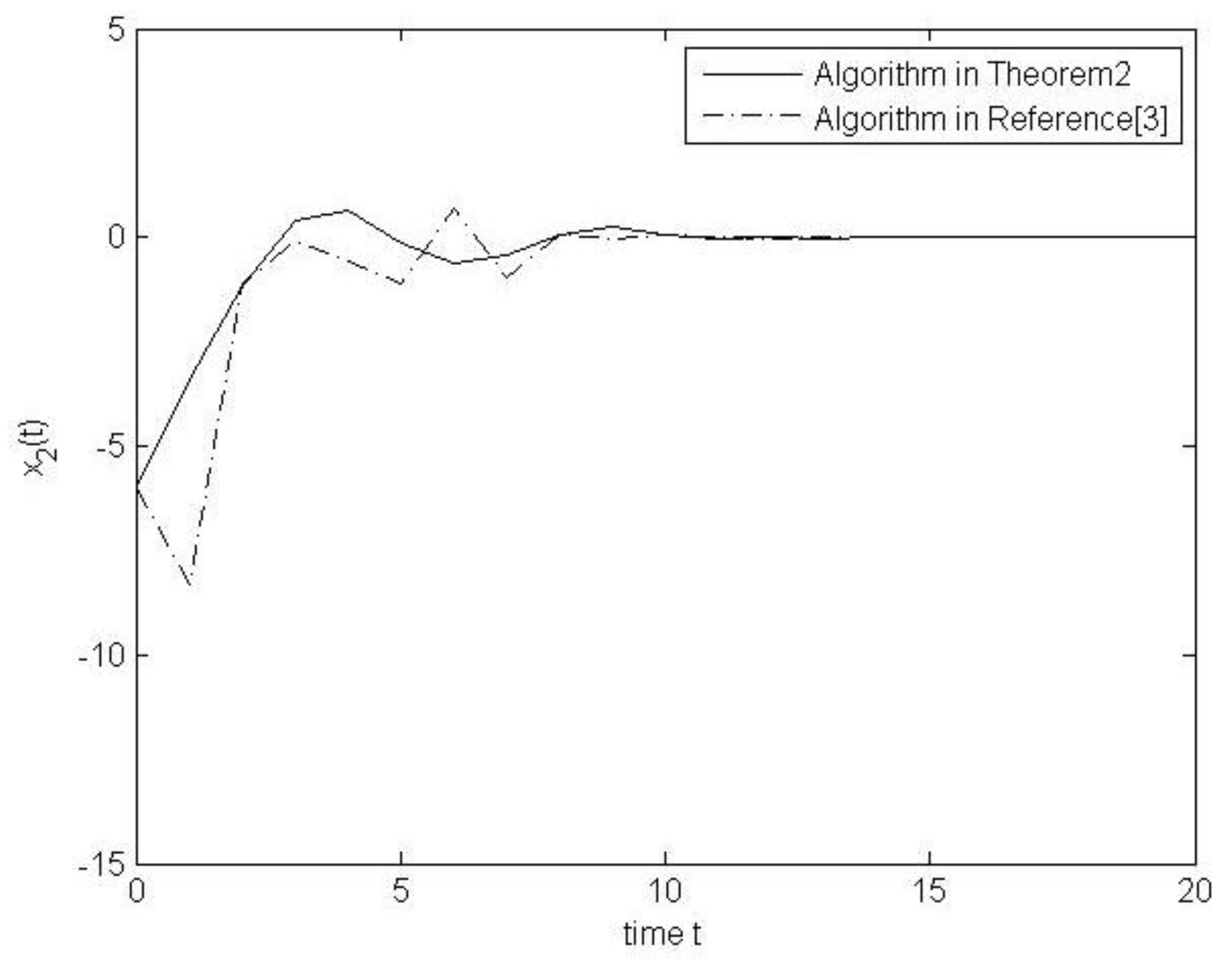
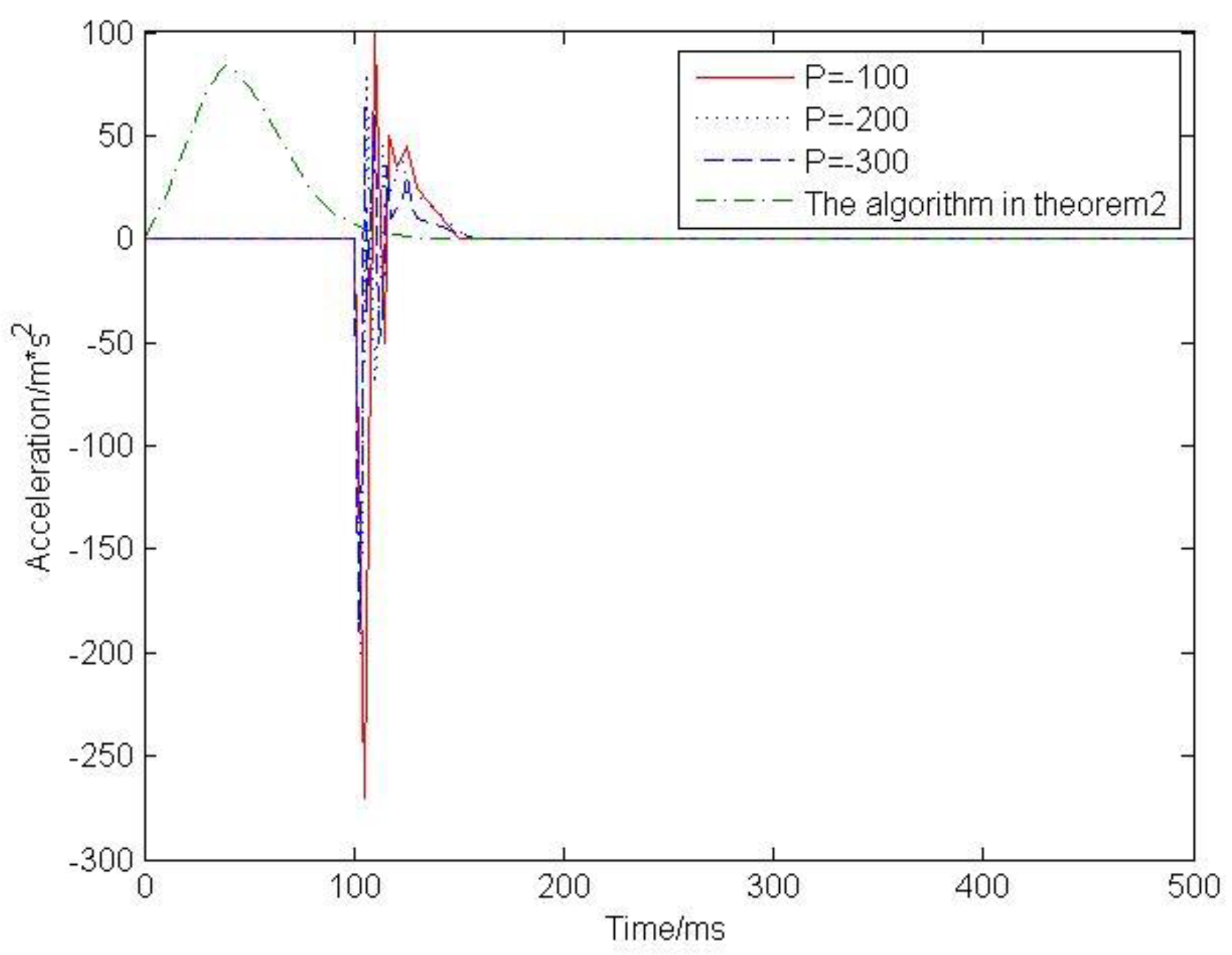
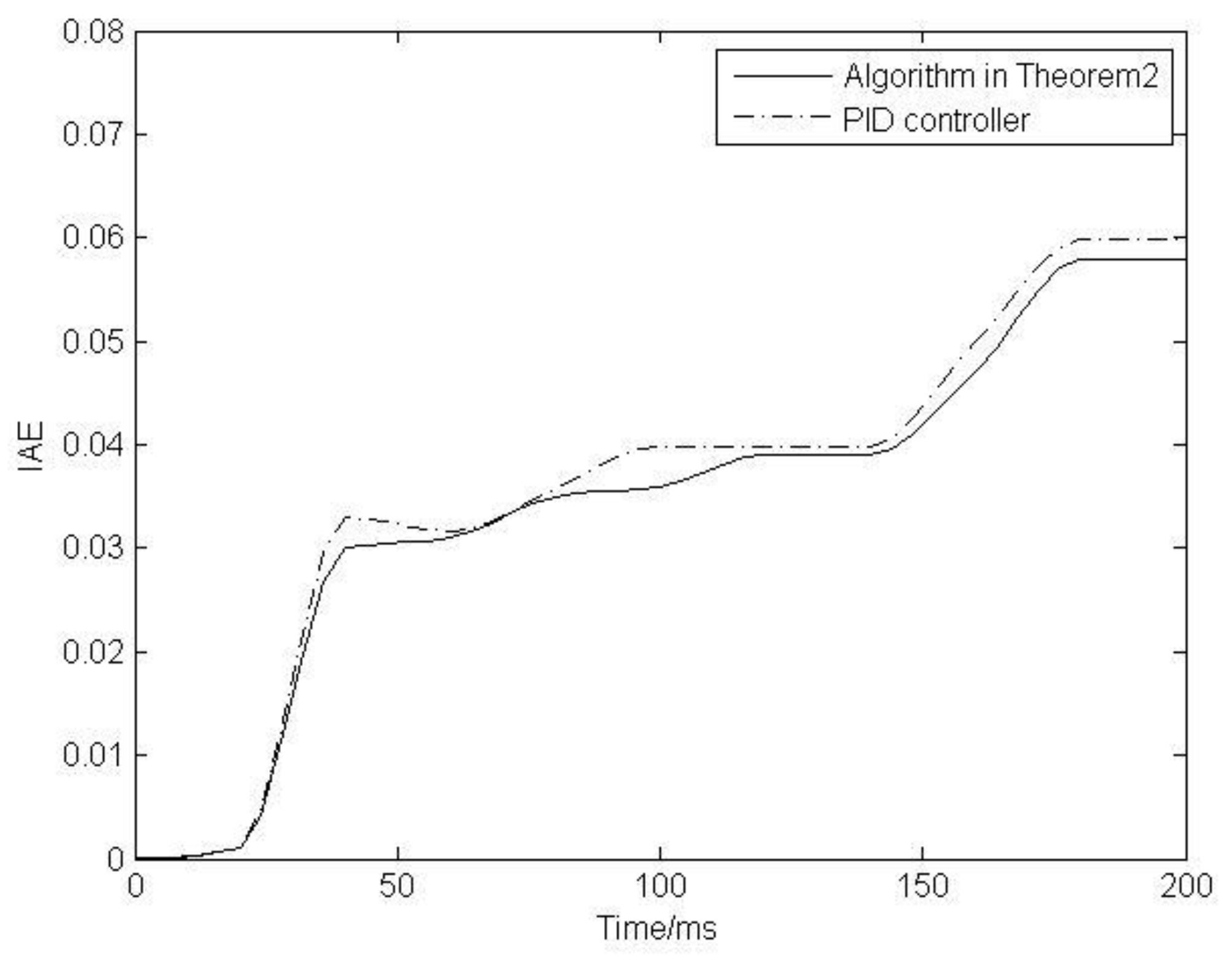
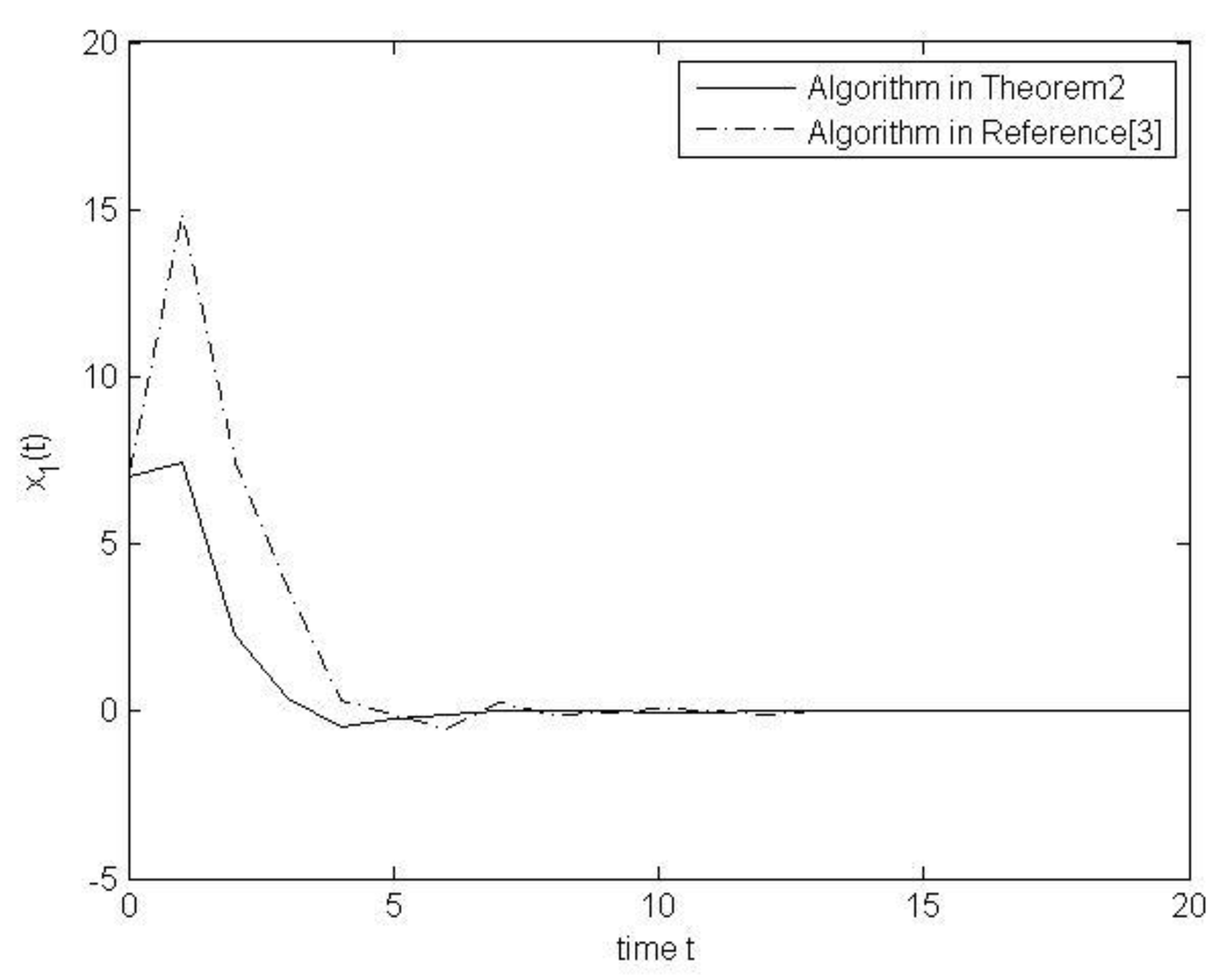
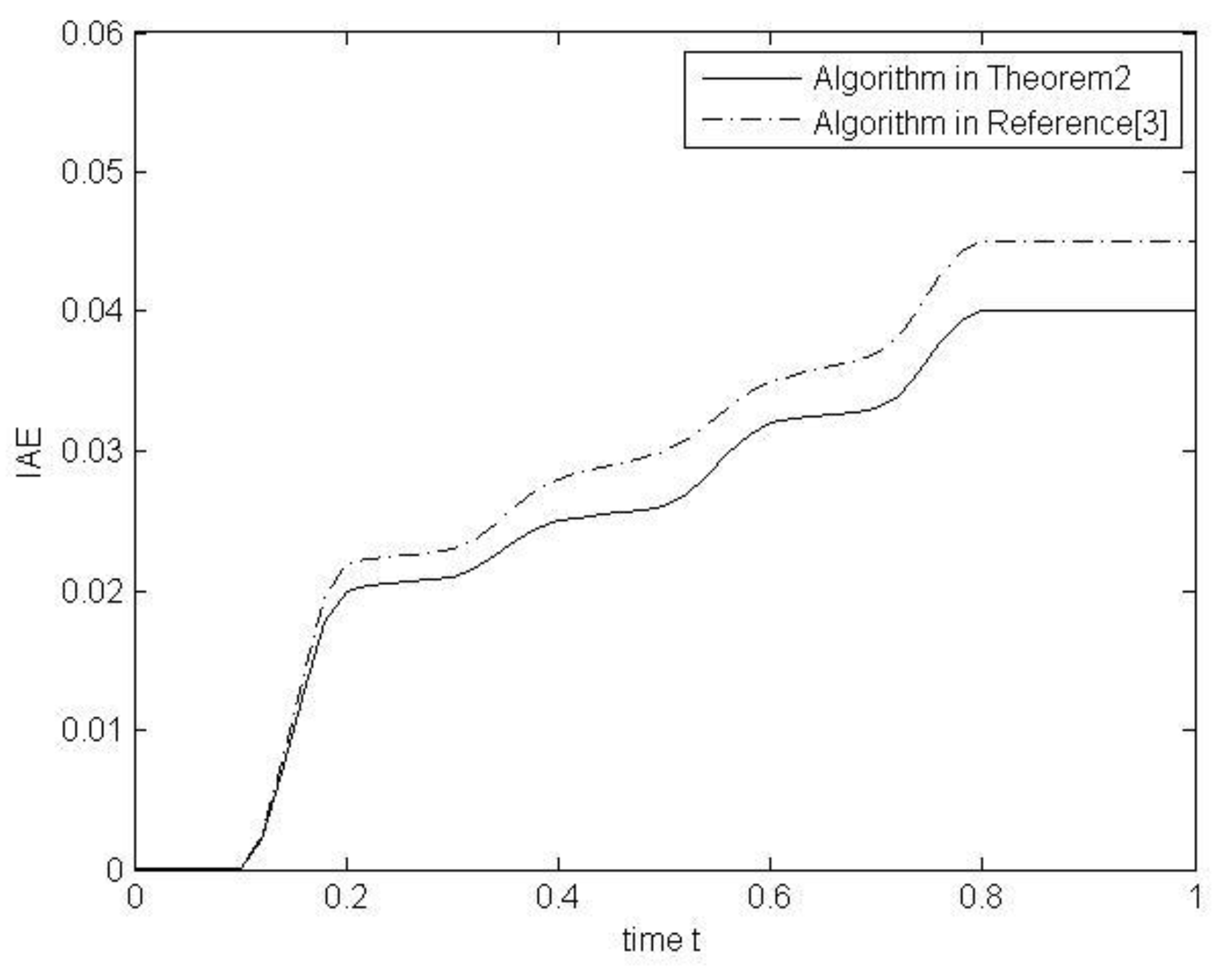
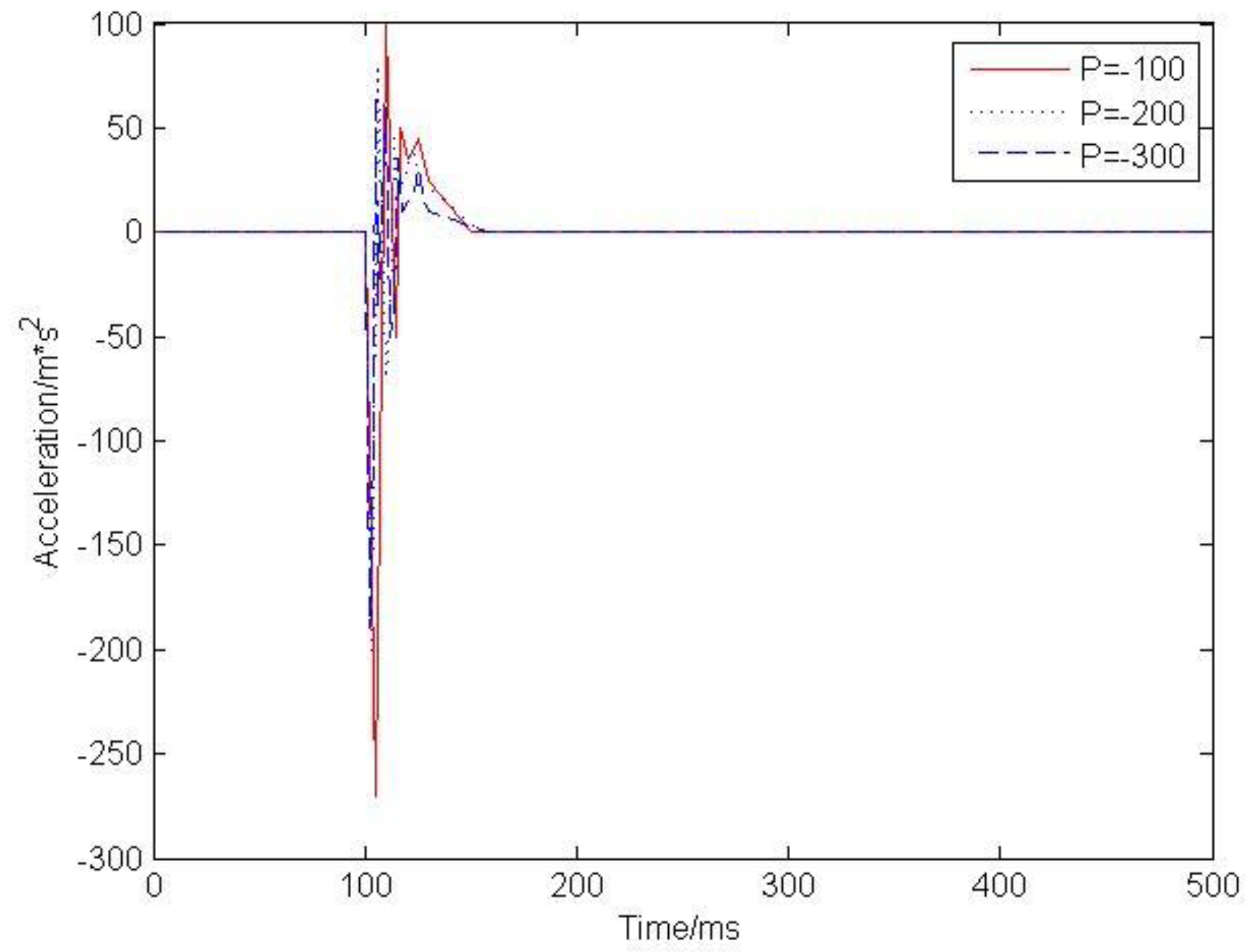
4. Simulation Examples

Example 1.

Consider the following saturated constrained time-delay systems (4), in order to compare with reference [3], some aspects have to be specified:

$$A=\left[\begin{array}{cc}0& 1\\ 0.3& 0\end{array}\right],A_d=\left[\begin{array}{cc}0.1& 0.2\\ 0& 0.3\end{array}\right],B=\left[\begin{array}{c}0.2\\ 1\end{array}\right],D_1=D_2=D_3=0,d=0.1.$$

By using the Algorithm in reference [3], the controller can be obtained as:

$$u(t)=[2.3306-1.8232]x(t).$$

On the other hand, by using the proposed approach in this paper, we solve the linear matrix inequality (9), the state feedback controller can be obtained as:

$$u(t)=2Kx(t)=[1.4369-0.3481]x(t).$$

(1)  Comparison of systems states simulation results with two algorithms

By selecting the initial value condition such as:

$$x(0)=\left[\begin{array}{c}7\\ -6\end{array}\right].$$

the state $x_1(t),x_2(t)$ response curves of the systems are as in Figure 1 and Figure 2.

In the Figure 1 and Figure 2, the solid line is the response for the systems states with algorithm in Theorem 2. The dot-dashed line presents the response with the algorithm in reference [3]. From the faster behavior of the systems states, the algorithm in Theorem 2 is better than the algorithm in reference [3], and the smoothness of solid line is also better than that of dashed line. Therefore, the algorithm in Theorem 2 presents better results than the algorithm in reference [3].

(2)  Verification of the systems performance

In order to verify the system performance, the dispersed Integral of Absolute Error (IAE) function is used as performance indicators to evaluate the system performance, which is:

$$IAE={\displaystyle {\int }_0^{\infty }|e(t)|dt}$$

The curves of IAE function that use algorithm in Theorem 2 and the algorithm in reference [3] are shown in the Figure 3.

The solid line is the curve of the IAE function using the algorithm in Theorem 2, and the dotted line is the curve of the IAE function using the algorithm in reference [3]. As time goes on, the change using the algorithm in Theorem 2 is less than the change using the algorithm in reference [3], obviously. Therefore, the algorithm in Theorem 2 can improve the systems control performance effectively.

Example 2.

The 1/4 body active suspension system can be simplified to a 2 degree of freedom (2-DOF) vibration system with springs, dampers and actuators. According to Newton’s second law, the equation of motion for the active suspension model of 1/4 vehicle body is obtained as follows:

$$\begin{array}{l}{m}_1{\ddot{X}}_1=K_1(X_2-X_1)+b({\dot{X}}_2-{\dot{X}}_1)+u\\ m_2{\ddot{X}}_2=-K_1(X_2-X_1)-b({\dot{X}}_2-{\dot{X}}_1)+K_2(X_0-X_2)-u\end{array}$$

(10)

where$m_1,m_2$are respectively the upper and lower mass of the spring, $K_1,K_2$are the suspension spring stiffness and tire stiffness respectively, $b$is the equivalent suspension damping coefficient, $u$is the acting force produced by the actuator, $X_1,X_2$are vertical displacement of body and suspension respectively, and$X_0$is the road input.

Selecting Vertical Displacement$X_1$of Car Body, Suspension vertical displacement$X_2$, Vehicle body vertical velocity${\dot{X}}_1$and Vertical Speed with Suspension${\dot{X}}_2$as the state variable$x$$x={\left[\begin{array}{cccc}{X}_1& X_2& {\dot{X}}_1& {\dot{X}}_2\end{array}\right]}^T$. Selection of control input vector$u^{\prime }={\left[\begin{array}{cc}u& X_0\end{array}\right]}^T$.

The output performance of suspension can be determined according to the vehicle ride comfort evaluation index. The ride comfort is usually evaluated by weighted acceleration root mean square value$(a_w)$, from which$y={\left[\begin{array}{cc}{\ddot{X}}_1& {\ddot{X}}_2\end{array}\right]}^T$is selected as the control output. From this, the following state equation and output equation are established:

$$\begin{array}{l}\dot{x}=Ax+B{u}^{\prime }\\ y=Cx+D{u}^{\prime }\end{array}$$

where

$$A=\left[\begin{array}{cccc}0& 0& 1& 0\\ 0& 0& 0& 1\\ -\frac{k_1}{m_1}& \frac{k_1}{m_1}& -\frac{b}{m_1}& \frac{b}{m_1}\\ \frac{k_1}{m_2}& \frac{-k_1-k_2}{m_2}& \frac{b}{m_2}& -\frac{b}{m_2}\end{array}\right],B=\left[\begin{array}{cc}0& 0\\ 0& 0\\ \frac{1}{m_1}& 0\\ -\frac{1}{m_2}& \frac{k_2}{m_2}\end{array}\right]$$

$$C=\left[\begin{array}{cccc}-\frac{k_1}{m_1}& \frac{k_1}{m_1}& -\frac{b}{m_1}& \frac{b}{m_1}\\ \frac{k_1}{m_2}& \frac{-k_1-k_2}{m_2}& \frac{b}{m_2}& -\frac{b}{m_2}\end{array}\right],D=\left[\begin{array}{cc}\frac{1}{m_1}& 0\\ -\frac{1}{m_2}& \frac{k_2}{m_2}\end{array}\right]$$

According to the theoretical analysis of the 1/4 body active suspension model and the saturated output characteristics of the actuator, an example is simulated by using MATLAB through the Proportion Integration Differentiation (PID) control method. The parameters of active suspension used for modeling and simulation are as follows: $m_1=225 \mathrm{kg}, m_2=30 \mathrm{kg}, k_1=18,500 \mathrm{N}/\mathrm{m}, k_2=1600 \mathrm{N}/\mathrm{m}, b=1600 \mathrm{N}\times \mathrm{s}/\mathrm{m}$, the step signal is used as the input for pavement.

Figure 4 shows the relationship between mass output acceleration and time on the spring of a 1/4 body active suspension model controlled by PID. Considering that proportional link (P) has the greatest impact on the whole system, this paper mainly analyzed the influence of PID control on active suspension by changing P values. When P = −100, −200 and −300, the relationship between simulation acceleration and time of suspension model is described in Figure 4.

Figure 4 shows that the maximum amplitude range of suspension output decreases with the increase of P absolute value. By adjusting the P value, PID control can effectively absorb the vibration output of suspension in this system. However, as the absolute value of P increases gradually, the frequency of system vibration also tends to increase, which makes the convergence time of the system increase and the stability of the system worse. Therefore, the PID control can effectively absorb the vibration output of the suspension, but it cannot guarantee the convergence speed of the system.

In order to compare the simulation results of systems states with PID controller, we used the proposed approach in this paper. Solving the linear matrix inequality (9), we get the state feedback controller:

$$u(t)=2Kx(t)=[-4.3472 0.2592]x(t).$$

The Relation response curve between Acceleration and Time is as in Figure 5.

From the Figure 5, one can see that the faster behavior and the smoothness of the curve of the Acceleration are better than that of PID controller. The results show that the proposed controller can improve the dynamic performance of the systems. The algorithm in Theorem 2 is better than the PID controller.

In order to compare the systems performance, the curves of the IAE function of the two algorithms are drawn in Figure 6.

The solid line is the curve of the IAE function using the algorithm in Theorem 2, and the dotted line is the curve of the IAE function using PID controller. Obviously, the algorithm in Theorem 2 is better than the PID controller.

5. Conclusions

In this paper, the asymptotic stability condition and state feedback control design method for the class of time-delay systems with actuator saturation are presented. By introducing a parameter matrix into the Lyapunov function, the conservativeness of the stability condition of the system is reduced.

References

1. Fuller, A.T. In the large stability of relay and saturating control systems with linear controllers. Int. J. Control 1969, 10, 457–480. [Google Scholar] [CrossRef]
2. Wang, C.L. Semi-global practical stabilization of nonholonomic wheeled mobile robots with saturated inputs. Automatica 2008, 44, 816–822. [Google Scholar] [CrossRef]
3. Joao, M.; Gomes, D.; Silva, J.; Sophie, T.; Germain, G. Anti-windup design for time-delay systems subject to input saturation an LMI-based approach. Eur. J. Control 2006, 12, 622–634. [Google Scholar]
4. Hu, T.; Lin, Z.; Chen, B.M. Analysis and design for discrete-time linear systems subject to actuator saturation. Syst. Control Lett. 2002, 45, 97–112. [Google Scholar] [CrossRef]
5. Zhou, R.; Zhang, X.; Shi, G. Output feedback stabilization of networked systems subject to actuator saturation and packet dropout. Lect. Notes Electr. Eng. 2012, 136, 149–154. [Google Scholar]
6. Zhao, L.; Xu, H.; Yuan, Y.; Yang, H. Stabilization for networked control systems subject to actuator saturation and network-induced delays. Neurocomputinng 2017, 267, 354–361. [Google Scholar] [CrossRef]
7. Song, Y.; Fang, X. Distributed model predictive control for polytopic uncertain system with randomly occurring actuator saturation and package losses. IET Control Theory Appl. 2014, 8, 297–310. [Google Scholar] [CrossRef]
8. Chen, Y.; Fei, S.; Li, Y. Stabilization of neutral time-delay systems with actuator saturation via auxiliary time-delay feedback. Automatica 2015, 52, 242–247. [Google Scholar] [CrossRef]
9. Zhou, B. Analysis and design of discrete-time linear systems with nested actuator saturations. Syst. Control Lett. 2013, 62, 871–879. [Google Scholar] [CrossRef]
10. Zhang, L.; Boukas, E.; Haidar, A. Delay-range-dependent control synthesis for time-delay systems with actuator saturation. Automatica 2008, 44, 2691–2695. [Google Scholar] [CrossRef]
11. Ma, Y.; Jia, X.; Zhang, Q. Robust observer-based finite-time H control for discrete-time singular Markovian jumping system with time delay and actuator saturation. Nonlinear Anal. Hybrid Syst. 2018, 28, 1–22. [Google Scholar] [CrossRef]
12. Ma, Y.; Jia, X.; Zhang, Q. Robust finite-time non-fragile memory H control for discrete-time singular Markovian jumping systems subject to actuator saturation. J. Frankl. Inst. 2017, 354, 8256–8282. [Google Scholar] [CrossRef]
13. Qi, W.; Kao, Y.; Gao, X.; Wei, Y. Controller design for time-delay system with stochastic disturbance and actuator saturation via a new criterion. Appl. Math. Comput. 2018, 320, 535–546. [Google Scholar] [CrossRef]
14. Song, G.; Lam, J.; Xu, S. Quantized feedback stabilization of continuous time-delay systems subject to actuator saturation. Nonlinear Anal. Hybrid Syst. 2018, 30, 1–13. [Google Scholar] [CrossRef]
15. Tao, Y.; Wei, H.; Zhao, Y. A dynamic allocation strategy of bandwidth of networked control systems with bandwidth constraints. Adv. Inf. Manag. Commun. Electron. Autom. Control 2017, 25, 1153–1158. [Google Scholar]
Figure 1. The state x 1 ( t ) response curves of the systems.
Symmetry 11 00375 g001
Figure 2. The state x 2 ( t ) response curves of the systems.
Symmetry 11 00375 g002
Figure 3. The curves of Integral of Absolute Error (IAE) of the two algorithms.
Symmetry 11 00375 g003
Figure 4. The Relation between Acceleration and Time at Different P Values.
Symmetry 11 00375 g004
Figure 5. The Relation between Acceleration and Time.
Symmetry 11 00375 g005
Figure 6. The curves of IAE of the two algorithms.
Symmetry 11 00375 g006