An Integrated Decision-Making Method Based on Neutrosophic Numbers for Investigating Factors of Coastal Erosion

Abstract

The recent boom of various integrated decision-making methods has attracted many researchers to the field. The recent integrated Analytic Network Process and Decision Making Trial and Evaluation Laboratory (ANP–DEMATEL) methods were developed based on crisp numbers and fuzzy numbers. However, these numbers are incapable of dealing with the indeterminant and inconsistent information that exists in real-life problems. This paper proposes improvements to the integrated ANP–DEMATEL method by bringing together the neutrosophic numbers, the ANP method, and the DEMATEL method, which are later abbreviated to NS-DANP. The proposed NS-DANP method can handle the indeterminacy elements in the decision-making environment, as the single-valued neutrosophic numbers are used in the decision analysis. This proposed NS-DANP modification method includes linguistic variables representing the single-valued neutrosophic numbers (SVNNs), and also introduces the single-valued neutrosophic weighted averaging (SVNWA) aggregation operator to aggregate the decision makers’ judgments instead of the typical averaging method. The applicability of the proposed method is illustrated by a case study of the coastal erosion problem along the Peninsular Malaysia coastline, where 12 factors were considered. Three experts of coastal erosion from different organizations were invited to elicit their linguistic judgments on the cause–effect of the coastal erosion. The seven-step decision approach was developed to acquire the weightage of each coastal erosion factor. The outcome of this study reveals that coastal development is the riskiest factor toward coastal erosion. The weight of factors and the cause–effect diagram could be very helpful for government and stakeholders to project a better mitigation plan for the coastal erosion problem. Comparative analysis is also provided to check the feasibility of the proposed method.

1. Introduction

Real-world problems involving multiple attributes and alternatives can only be solved using multi-criteria decision making (MCDM) tools. There are many well-known MCDM methods in the decision-making field; for instance, the Analytic Hierarchy Process (AHP), Analytic Network Process (ANP), the Technique for Order of Preference by Similarity to Ideal Solution (TOPSIS), VlseKriterijumska Optimizacija I Kompromisno Resenje technique (VIKOR), Elimination and Choice Expressing Reality (ELECTRE), Grey Relational Analysis (GRA), Preference Ranking Organization Method for Enrichment of Evaluations (PROMETHEE), Decision Making Trial and Evaluation Laboratory (DEMATEL), and a hybrid of MCDM methods. Every MCDM method has its own specialty and advantages for solving complicated real problems. As for clarifying the interrelationships of criteria, the DEMATEL method is the best method that has been developed for this purpose. The DEMATEL method was developed by the Science and Human Affairs Program of the Battelle Memorial Institute of Geneva, and has been well-known for its capability in dealing with the degree of importance of evaluation criteria, and more importantly to build cause–effect relationships among the evaluation criteria [1]. By pairwise comparisons of the interactions among criteria, the method utilizes matrix operations and mathematical techniques to quantify the causality and confirm the interdependence among criteria [2]. The causal diagram portrays a clear causal relationship and the degree of influence among the criteria. Recently, several studies have employed the DEMATEL method in various problems, such as those regarding cloud service selection [3], business intelligence [4], health technology assessment [5], the performance of a manufacturing company [6], supply chain [7,8], coastal erosion [9], and the auto components manufacturing sector [10].

One of the established MCDM tools for handling the feedback and dependencies among criteria and clusters is ANP [11]. The ANP method was introduced by Saaty [12] to avoid the hierarchical constraint in the analytic hierarchy process (AHP). Furthermore, the ANP method is used to determine the composite weights of the criteria through the development of a ‘supermatrix’ [13]. The supermatrix is actually a partitioned matrix that represents a relationship between two clusters in a system [14]. In addition to this, along the process of obtaining the final weights, arrays of elements in a matrix are used to easily convey the mechanisms of the methodology and show how dependencies function [15]. Therefore, the supermatrix is the better option, especially when involving a greater number of elements. However, there are a few flaws in the standalone ANP method. One of them is the assumption that each cluster has the same weight. This assumption is not sensible, since the weight of each cluster has a high possibility of being different from each other. Another shortcoming of ANP is that the assessment survey involves too many pairwise comparisons. This may lead to inconsistent judgment, which is time consuming and difficult to interpret. Therefore, the hybridization of DEMATEL and ANP methods has been widely explored, and has been recognized for supporting the imperfections in the solely ANP method.

Besides the combination of the DEMATEL–ANP methods, there are several integrations that promote DEMATEL that have been explored, such as the hybrid of AHP and DEMATEL [16], DEMATEL and TOPSIS [17], grey-based DEMATEL [18], DEMATEL and adaptive neuro-fuzzy inference systems (ANFIS) [6], DEMATEL and fuzzy inference system (FIS) [19], DEMATEL and VIKOR [20], DEMATEL and data envelopment analysis (DEA) [21], DEMATEL–ANP with DEA [22,23], DEMATEL, ANP, and PROMETHEE II [24], DEMATEL with ANP and the Multi-Attributive Ideal-Real Comparative Analysis (MAIRCA) method [25], DEMATEL with ANP and ELECTRE [26], DEMATEL with ANP and VIKOR [27], DEMATEL with ANP, GRA, and VIKOR [28], and DEMATEL with ANP and TOPSIS [29].

Generally, ANP studies comprise three main components, which are the network structuring of the problem, coping with inner and outer dependencies through the pairwise comparison, and forming the weighted supermatrix. According to Baykasoklu and Golcuk [30], there are four types of integrated DEMATEL–ANP technique in the literature. The first category employs DEMATEL merely for structuring the network relationship map (NRM). The inner and outer dependencies and weighted supermatrix are obtained via the traditional ANP method. The second category utilizes DEMATEL to deal with the inner dependencies. The criteria structuring, the outer dependencies, and the weighted supermatrix are accomplished using the ANP method. This category benefits from avoiding the difficulty of pairwise comparison of the ANP method. The third category adopts DEMATEL for obtaining the clusters’ weights and constructing the NRM. The inner and outer dependencies are handled via the ANP method. The main purpose of this category is to incorporate the unequal weights of clusters into the formation of the supermatrix. Lastly, the fourth category uses DEMATEL in establishing the NRM, handling inner and outer dependencies and weighted supermatrix formation. This type of hybridization generalizes the previous mentioned categories and is well-known as the DANP method.

However, most of the DANP method only uses the real number in their computation methodology. Since the introduction of the fuzzy set (FS) theory by Zadeh [31], the studies related to this theory have been explored widely, and its real applications have been successfully implemented in various fields, including fuzzy DEMATEL [32,33], fuzzy ANP [34,35], and fuzzy DEMATEL–ANP [36,37]. The fuzzy DEMATEL, for instance, is superior to the traditional DEMATEL method, because it uses linguistic variables that represent fuzzy numbers in the evaluation processes instead of integer numbers from zero to four. Fuzzy numbers (FN) are well-known numbers in an uncertain environment owing to its ability to handle uncertain information. As a result, many researchers have utilized the DEMATEL method in a fuzzy environment and used triangular fuzzy numbers (TFNs) in its method development [38,39]. Despite its capability, there is one weakness when applying TFNs into the DEMATEL method, which has been pointed out by Pandey and Kumar [40]. According to Pandey and Kumar [40], the computation of a multiplicative inverse of fuzzy matrix in the DEMATEL method is invalid, because the elements in the matrix are dependent with each other, and thus the computation of the multiplicative inverse of the fuzzy matrix cannot be implemented separately. These flaws can be seen in many studies that apply the TFNs into DEMATEL methods: [32,41,42] just to cite a few. Besides TFNs, DEMATEL is applied with other sets such as trapezoidal FS [43], type-2 FS [44], interval type-2 FN [16,45], intuitionistic fuzzy sets (IFS) [46,47,48], interval rough sets [25], hesitant fuzzy linguistic term sets [49], and an interval-valued hesitant fuzzy set [50].

Besides that, the traditional FN only expresses one single value of membership function, ${\mu }_A\left(x\right)\in \left[0,1\right]$ of fuzzy set A. However, in most of the real applications such as an expert system, information fusion, and a belief system, we should not only consider truth-membership, but also falsity-membership [51]. Therefore, Atanassov [52] introduced intuitionistic fuzzy sets (IFSs), which extend the concept of FS by adding the degree of non-membership. Since its introduction, IFS has received significant interest among scholars, and lots of remarkable studies have been executed on developing theories of IFSs. Later, Atanassov and Gargov [53] introduced interval-valued IFS (IVIFS), which uses interval values to represent the degrees of membership and non-membership, instead of just real numbers. However, FSs, IFSs, and IVIFSs are incapable of dealing with all the types of uncertainty that exist in different real-life problems, especially when it involves indeterminant and inconsistent information. In IFSs, the indeterminacy degree, or the so-called hesitancy degree in IFS literature can be obtained by default, which is $1-{\mu }_A\left(x\right)-{\nu }_A\left(x\right)$.

When we asked a decision maker (DM) about his or her opinion on a certain statement, he or she may evaluate the statement with three possibilities. First, he or she may state that the truthness of that statement is 0.5. Second, he or she may elicit that the degree of falsity is 0.6, and third, that the degree of unsure is 0.2, which is beyond the scope of FSs, IFSs, and IVIFSs [51]. In a neutrosophic set (NS), indeterminacy is quantified explicitly, which means that the truth, falsity, and indeterminacy components are completely independent. NS is a set that was introduced by Smarandache [54] where each element has the degree of truth, falsity, and indeterminacy, and it is within the non-standard unit interval of $\left]0^{-},1^{+}\right[$. This set is clearly an extension from the standard unit interval of IFS, $\left[0,1\right]$. However, the non-standard unit of NSs are difficult to be applied in the real-case situations; therefore, Wang et al. [51] presented the notion of single-valued neutrosophic set (SVNS), which is a special case of NSs. Since its introduction, the SVNS has attracted many scholars to theoretically improve the set by introducing new concepts of measures, defining operations, aggregation operators, and correlation coefficients associated to the set [55,56,57,58]. It also has been successfully applied in various MCDM problems such as in logistics center location selection [59], teacher selection problem [60], medical diagnosis [61], etc.

The successful applications of neutrosophic numbers, especially SVNSs in the MCDM-related problems, motivated us to explore the possibility of the development of an integrated neutrosophic DEMATEL-based ANP (NS-DANP). The acronym NS-DANP will be used throughout this paper. The introduction of SVNSs in the DEMATEL method would enhance the efficiency in handling the uncertainty and indeterminacy information that exists during the pairwise comparison evaluation process. In addition, to the best of our knowledge, there are no studies in the previous literature that used neutrosophic sets in an integrated DEMATEL and ANP method. In contrast to the other ANP–DEMATEL methods, this proposed NS-DANP method makes the computation a lot easier, as it generalizes the other hybrid ANP–DEMATEL methods. In addition, comparative analysis is carried out to show the applicability and effectiveness of the proposed NS-DANP method under a single valued neutrosophic environment compared to other existing methods. It is consistent with most of the past research in decision analysis, where comparative analysis was made to compare their proposed methods with existing methods [62,63,64].

This paper has twofold purposes. First, we aim to introduce the SVNSs into the DEMATEL method, as they are superior to traditional FSs, and avoid the multiplicative inverse problem in the fuzzy DEMATEL method. Secondly, to test the applicability of the proposed method, it is applied to a case study of coastal erosion problem along the Peninsular Malaysia coastal area. The rest of the paper is as follows. The second section discusses the preliminaries. The third section explains the proposed integrated neutrosophic DEMATEL-based ANP method (NS-DANP). Then, we provide a case study where the coastal erosion problem is implemented using the proposed methodology. The next section is continued with the comparative analysis. The last section concludes.

2. Preliminaries

This section provides some basic definitions of NSs, SVNSs, the weights of decision makers (DMs), the deneutrosophication of single-valued neutrosophic numbers, and the single-valued neutrosophic weighted averaging (SVNWA) aggregation operator.

Definition 1

([54]). Let $X$ be a space of points, with generic elements in $X$ denoted by $x$. A neutrosophic set $Q$ in $X$ is denoted by $Q=\left\{\langle x,T_Q\left(x\right),I_Q\left(x\right),F_Q\left(x\right)\rangle |x\in X\right\}$ where $T_Q\left(x\right)$ is the truth-membership function, $I_Q\left(x\right)$ is the indeterminacy-membership function, and $F_Q\left(x\right)$ is the falsity-membership function. The functions $T_Q\left(x\right),I_Q\left(x\right)$ and $F_Q\left(x\right)$ are real standard subsets of $\left]0^{-},1^{+}\right[$. That is, $T_Q\left(x\right),I_Q\left(x\right),F_Q\left(x\right)\to \left]0^{-},1^{+}\right[$. Thus, the sum of $T_Q\left(x\right),I_Q\left(x\right)$ and $F_Q\left(x\right)$ is $0^{-}\le \sup T_Q\left(x\right)+\sup I_Q\left(x\right)+\sup F_Q\left(x\right)\le 3^{+}$.

Obviously, the non-standard subsets are difficult to be applied in real scientific and engineering areas. Hence, Wang et al. [51] presented the SVNS and defined it as follows.

Definition 2.

Let$X$be a space of points (objects) with generic elements in$X$denoted by$x$. An SVNS$Q$can be denoted by$Q=\left\{\langle x,T_Q\left(x\right),I_Q\left(x\right),F_Q\left(x\right)\rangle |x\in X\right\}$where$T_Q\left(x\right)$is the truth-membership function,$I_Q\left(x\right)$is the indeterminacy-membership function, and$F_Q\left(x\right)$is the falsity-membership function. That is,$T_Q\left(x\right),I_Q\left(x\right),F_Q\left(x\right)\to \left[0,1\right]$for each point$x$in$X$, and the sum of$T_Q\left(x\right),I_Q\left(x\right)$and$F_Q\left(x\right)$satisfies the condition$0\le T_Q\left(x\right)+I_Q\left(x\right)+F_Q\left(x\right)\le 3$.

The weight of DMs may be distinct from each other. The DM’s weights can be obtained by the following definition [65].

Definition 3.

Let$Q_m=\langle T_m,I_m,F_m\rangle$ be an SVNS defined for the rating of the m-th DM. Then, the weight of the m-th DM can be written as:

$${\omega }_m=\frac{1-\sqrt{\left\{{\left(1-T_m\right)}^2+{\left(I_m\right)}^2+{\left(F_m\right)}^2\right\}/3}}{{\displaystyle {\sum }_{m=1}^p\left(1-\sqrt{\left\{{\left(1-T_m\right)}^2+{\left(I_m\right)}^2+{\left(F_m\right)}^2\right\}/3}\right)}}$$

(1)

Further, in any decision analysis, the consensus decision making is the important key in achieving a promising solution. In this regard, the formation of an aggregated decision matrix is a must where all the individual DMs’ judgments are aggregated. By incorporating the weights of DMs in Definition 3, the aggregated SVNS decision matrix can be computed using the SVNWA aggregation operator defined in Definition 4 [66].

Definition 4.

Let$A^{\left(m\right)}={\left(a_{ij}^{\left(m\right)}\right)}_{n\times n}$be the individual SVNS decision matrix of the m-th DM and$\omega ={\left({\omega }_1,{\omega }_2,\dots ,{\omega }_p\right)}^T$be the weight vector of DM such that each${\omega }_m\in \left[0,1\right]$. $A={\left(a_{ij}\right)}_{n\times n}$, where

$$a_{ij}=SVNW{A}_{\omega }\left(a_{ij}^{\left(1\right)},a_{ij}^{\left(2\right)},\dots ,a_{ij}^{\left(p\right)}\right)$$

$$={\omega }_1{a}_{ij}^{\left(1\right)}\oplus {\omega }_2{a}_{ij}^{\left(2\right)}\oplus \dots \oplus {\omega }_p{a}_{ij}^{\left(p\right)}$$

$$=\langle 1-{{\displaystyle \prod _{m=1}^p\left(1-T_{ij}^{\left(m\right)}\right)}}^{{\omega }_m},{\displaystyle \prod _{m=1}^p{\left(I_{ij}^{\left(m\right)}\right)}^{{\omega }_m},{\displaystyle \prod _{m=1}^p{\left(F_{ij}^{\left(m\right)}\right)}^{{\omega }_m}}}\rangle$$

(2)

Deneutrosophication is the process of obtaining one single real number from any of the neutrosophic numbers. The deneutrosophication of SVNNs is defined as below [65].

Definition 5.

Let$Q=\left\{\langle x,T_Q\left(x\right),I_Q\left(x\right),F_Q\left(x\right)\rangle |x\in X\right\}$be an SVNN, then the deneutrosophication of$Q$is the process of set$Q$mapping into a real number$\chi \in X$i.e.,$f:Q\to \chi$for$x\in X$. The set$Q$is reduced to a crisp number$\chi \in X$. Therefore, the deneutrosophication can be computed as Equation (3).

$${\chi }_Q=1-\sqrt{\left\{{\left(1-T_Q\left(x\right)\right)}^2+{\left(I_Q\left(x\right)\right)}^2+{\left(F_Q\left(x\right)\right)}^2\right\}/3}$$

(3)

3. Proposed Method

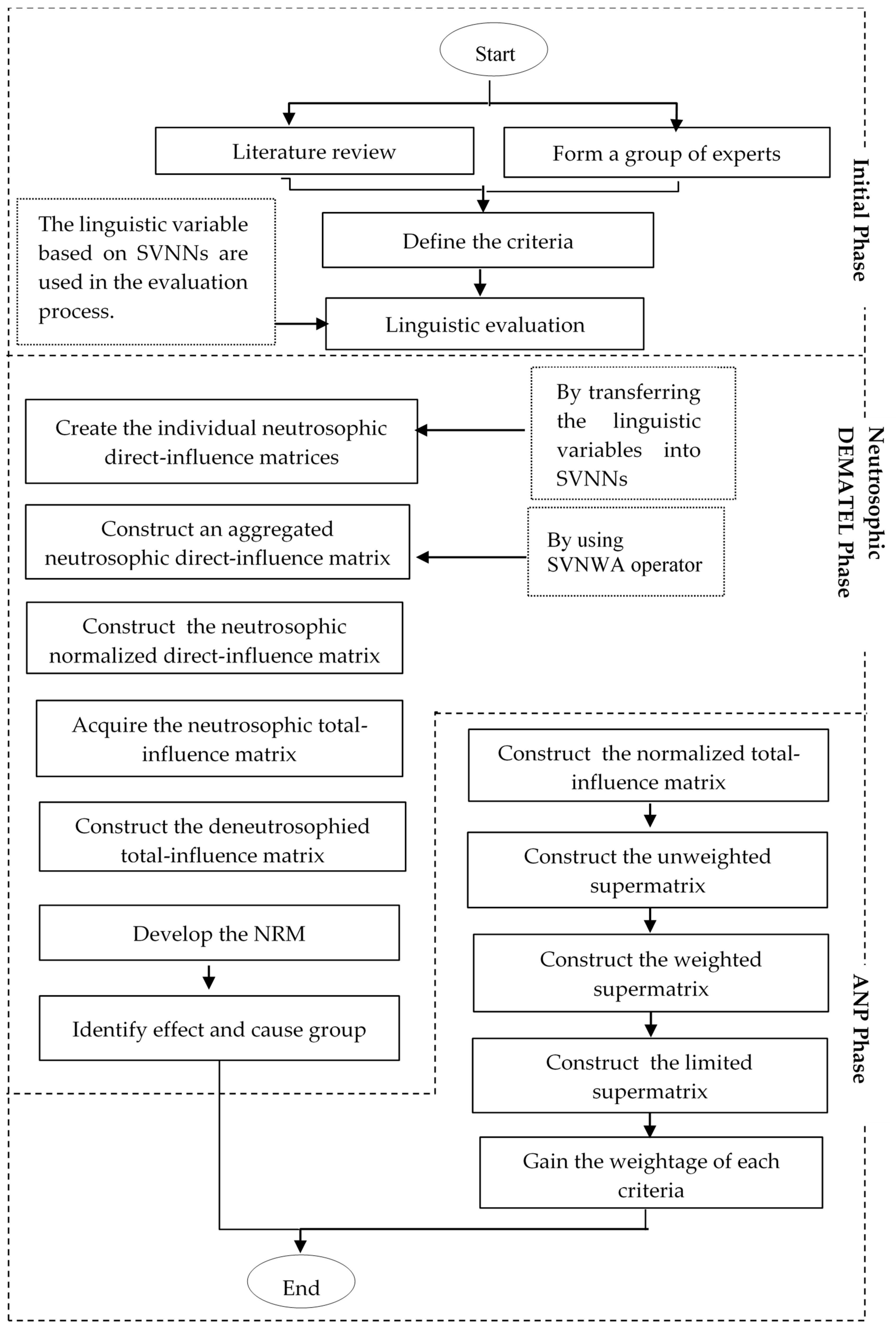
The DANP hybrid technique with SVNSs (NS-DANP) is adopted in this study. The NS-DANP approach does not only apply neutrosophic DEMATEL to obtain the NRM and the degree of influences of dimensions and criteria. Instead, the NS-DANP that is incorporated normalizes the total-influence matrix T of DEMATEL into an unweighted supermatrix of ANP. In addition, the relationships element reflected from the total-influence matrix of DEMATEL is similar to the idea of ANP, which supports the importance of criteria through questionnaires. Besides that, this proposed NS-DANP method is better than the integrated DEMATEL and AHP, because the AHP only considers the unidirectional interactions between components in the lower level of the hierarchy with respect to the components in upper level of the hierarchy, while the ANP method can handle the interactions among inner dependency, outer dependency, and self-feedback [30]. Therefore, the ANP is a practical tool to solve the real complex problem by integrating the key interrelationships of criteria in the form of the supermatrix. The supermatrix or influence matrix is a generalization of the AHP, since the ANP offers more flexible interactions among clusters and criteria. Development of the proposed NS-DANP method is carried out in three phases. The initial phase is where the collection of data is executed via the linguistic evaluation of DMs. The second phase analyzes the data using the developed neutrosophic DEMATEL method. The total-influence matrix of DEMATEL is incorporated into the ANP methodology in Phase 3 to get the influential weights of criteria. To highlight the new developed structure of the proposed NS-DANP method, the three phases are visualized as in Figure 1.

In the first phase, the questionnaire is developed, a group of experts is recognized, the dimensions and influencing criteria are finalized, and the linguistic variables are set to carry out the pairwise comparison evaluation and get the information for this study. After obtaining the data, the linguistic variable information is transformed into SVNSs in matrix form. The individual experts’ initial direct-influence matrices are aggregated using the SVNWA aggregation operator. This aggregation operator is introduced into this study, as it is easy to compute and efficient in aggregating SVNSs. Then, in the second phase, the DEMATEL method based on SVNS is implemented to develop the NRM and classify the influencing criteria into cause and effect groups. The third phase is where the integration between DEMATEL and ANP commences. The total-influence matrix obtained from the DEMATEL method is utilized in the ANP method. As a result of this NS-DANP integration, the weights of each influencing criteria are obtained. The individual steps of the proposed NS-DANP method are shown below.

Step 1. Establish the neutrosophic aggregated direct-influence matrix $A^G$.

In this step, each expert was asked to state the degree of direct influence based on the scale ranging from zero to four, which indicates the linguistic variable from “no influence” to “very high influence”. The linguistic variable is used in most of the MCDM evaluation process, because of the human language that is easy to be interpreted for gaining information from experts’ purposes.

Table 1. Linguistic variable and its corresponding single-valued neutrosophic numbers (SVNNs) [65].

Integer	Linguistic Variable	SVNNs
0	Very unimportant (VU)	$\langle 0.1,0.8,0.9\rangle$
1	Unimportant (U)	$\langle 0.35,0.6,0.7\rangle$
2	Medium important (M)	$\langle 0.5,0.4,0.45\rangle$
3	Important (I)	$\langle 0.8,0.2,0.15\rangle$
4	Absolutely important (AI)	$\langle 0.9,0.1,0.1\rangle$

shows the zero to four scale, the linguistic variables, and their corresponding SVNSs adopted from Biswas et al. [65].

The evaluation information obtained from each expert will be converted into the neutrosophic direct-influence matrix form. Since each expert produces an individual neutrosophic direct-relation matrix, a neutrosophic aggregated direct-relation matrix needs to be derived by the SVNWA aggregation operator using Equation (2). The weights of experts need to be calculated beforehand using Equation (1).

Hence, the neutrosophic aggregated direct-influence matrix, $A^G$, is denoted as below.

$$A^G=\left[\begin{array}{c}\begin{array}{ccc}{a}_{11}& \cdots & a_{1n}\end{array}\\ \begin{array}{ccc}⋮& \ddots & ⋮\end{array}\\ \begin{array}{ccc}{a}_{n1}& \cdots & a_{nn}\end{array}\end{array}\right],$$

where $a_{ij}$ is SVNSs with the form of $\langle T_{ij},I_{ij},F_{ij}\rangle$, and indicates the influence degree of factor i on factor j.

Step 2. Construct the neutrosophic normalized direct-influence matrix, B.

The neutrosophic normalized direct-influence matrix can be obtained through Equations (4) and (5).

$$B=k\times A^G,$$

(4)

$$\mathrm{where}k=\min \left[\frac{1}{\underset{i}{\max }{\displaystyle {\sum }_{j=1}^n{T}_{ij}}},\frac{1}{\underset{j}{\max }{\displaystyle {\sum }_{i=1}^n{T}_{ij}}}\right]$$

(5)

Step 3. Acquire the total direct-influence matrix, S.

For this step, the multiplicative inverse of $\left(I-B\right)$ matrices need to be calculated in order to get the total direct-influence matrices. In this regard, Pandey and Kumar [40] cautioned in their commenting paper that it was an invalid step for the computation of the multiplicative inverse of fuzzy matrices. This invalid inverse operation has been noticed in most of the previous articles when applying the fuzzy DEMATEL method [32,41,42]. In the fuzzy DEMATEL method, the multiplicative inverse of fuzzy matrices was done separately by its elements. This is invalid, since the elements of fuzzy numbers are dependent on each other. In this regard, this paper utilizes the neutrosophic numbers so as to divert the flaws that exist in the fuzzy DEMATEL method. Since the elements in neutrosophic sets are independent from each other, the multiplicative inverse of neutrosophic matrices can be done separately. The introduction of neutrosophic sets in DEMATEL is seen as the way to overcome the drawback in fuzzy DEMATEL methodology.

The matrix S can be obtained by the following equations:

$$S=B+B^2+\dots +B^k$$

$$=B\left(1+B+B^2+\dots +B^{k-1}\right)\left(1-B\right){\left(1-B\right)}^{-1}$$

$$=B\left(1-B^k\right){\left(1-B\right)}^{-1}$$

$$=B{\left(1-B\right)}^{-1}\mathrm{when}\underset{k\to \infty }{\lim }{B}^k={\left[0\right]}_{n\times n}$$

(6)

where $S={\left[s_{ij}\right]}_{n\times n}=\left[\begin{array}{c}\begin{array}{ccc}{s}_{11}& \cdots & s_{1n}\end{array}\\ \begin{array}{ccc}⋮& \ddots & ⋮\end{array}\\ \begin{array}{ccc}{s}_{n1}& \cdots & s_{nn}\end{array}\end{array}\right]$, and $s_{ij}=\langle T_{ij}\left(x\right),I_{ij}\left(x\right),F_{ij}\left(x\right)\rangle$, then

$$\mathrm{Matrix}\left[T_{ij}\right]=B_T{\left(I-B_T\right)}^{-1}$$

(7)

$$\mathrm{Matrix}\left[I_{ij}\right]=B_I{\left(I-B_I\right)}^{-1}$$

(8)

$$\mathrm{Matrix}\left[F_{ij}\right]=B_F{\left(I-B_F\right)}^{-1}$$

(9)

where I is the neutrosophic identity matrix with diagonal elements of $\langle 1,1,1\rangle$ and non-diagonal elements of $\langle 0,0,0\rangle$.

Then, the elements in matrix S is deneutrosophied to obtain crisp numbers. The deneutrosophication can be computed as Equation (3). From the deneutrosophied matrix S, the prominence and relation of each criterion can be derived by Equations (10) and (11):

$$a={\left(a_i\right)}_{n\times 1}={\left[{\displaystyle \sum _{j=1}^n{s}_{ij}}\right]}_{n\times 1}$$

(10)

$$b={\left(b_j\right)}_{1\times n}={\left[{\displaystyle \sum _{i=1}^n{s}_{ij}}\right]}_{1\times n}$$

(11)

where $a_i$ is the sum of rows of matrix S, and $b_j$ is the sum of columns of matrix S. The $\left(a_i+b_i\right)$ values indicate the importance of each criterion. The $\left(a_i-b_i\right)$ values can be categorized into two groups, which are the net receiver and net causer. The positive $\left(a_i-b_i\right)$ values indicate the criterion i affecting the other criterion, while if the $\left(a_i-b_i\right)$ value is negative, the criterion i is being influenced by the other criteria.

Step 4. Draw the network relationship map (NRM).

The NRM can be drawn by mapping $\left(a_i+b_i,a_i-b_i\right)$, which provides an understandable structure that clearly expresses the relationship among criteria, degree of influences, and impacts of each criterion. The threshold value is set to eliminate the small influences in matrix S. The threshold value is given by an expert based on their opinions. After verifying the interrelationship among dimensions and criteria by neutrosophic DEMATEL, the ANP method is incorporated to determine the influential weights of each criteria.

Step 5. Form the unweighted supermatrix.

The neutrosophic total-influence matrix for criteria obtained from the neutrosophic DEMATEL method is denoted by $S_c$.

$$\begin{array}{ccc}& & D_1 D_2 \cdots D_n\\ & & c_{n1}\dots c_{n{m}_n} c_{n1}\dots c_{n{m}_n} \cdots c_{n1}\dots c_{n{m}_n}\\ S_c=& \begin{array}{}\\ \\ D_1\\ \\ \\ D_2\\ \\ ⋮\\ \\ D_n\\ \\ \end{array}\begin{array}{c}\begin{array}{c}{c}_{11}\\ c_{12}\\ \begin{array}{c}⋮\\ c_{1m_1}\end{array}\end{array}\\ \begin{array}{c}{c}_{21}\\ c_{22}\\ \begin{array}{c}⋮\\ c_{2m_2}\end{array}\end{array}\\ ⋮\\ \begin{array}{c}{c}_{n1}\\ c_{n2}\\ \begin{array}{c}⋮\\ c_{n{m}_n}\end{array}\end{array}\end{array}& \left[\begin{array}{cccccccccc}{S}_c^{11}& & & & S_c^{12}& & & \cdots & & S_c^{1n}\\ \\ \\ \\ S_c^{21}& & & & S_c^{22}& & & \cdots & & S_c^{2n}\\ \\ ⋮& & & & ⋮& & & \ddots & & ⋮\\ \\ \\ S_c^{n1}& & & & S_c^{n2}& & & \cdots & & S_c^{nn}\end{array}\right]\end{array}$$

(12)

To obtain matrix $s_c^{\alpha }$, the matrix $S_c$ needs to be normalized by dimensions as shown in Equation (13):

$$\begin{array}{ccc}& & D_1 D_2 \cdots D_n\\ & & c_{n1}\dots c_{n{m}_n} c_{n1}\dots c_{n{m}_n} \cdots c_{n1}\dots c_{n{m}_n}\\ S_c^{\alpha }=& \begin{array}{}\\ \\ D_1\\ \\ \\ D_2\\ \\ ⋮\\ \\ D_n\\ \\ \end{array}\begin{array}{c}\begin{array}{c}{c}_{11}\\ c_{12}\\ \begin{array}{c}⋮\\ c_{1m_1}\end{array}\end{array}\\ \begin{array}{c}{c}_{21}\\ c_{22}\\ \begin{array}{c}⋮\\ c_{2m_2}\end{array}\end{array}\\ ⋮\\ \begin{array}{c}{c}_{n1}\\ c_{n2}\\ \begin{array}{c}⋮\\ c_{n{m}_n}\end{array}\end{array}\end{array}& \left[\begin{array}{cccccccccc}{S}_c^{\alpha 11}& & & & S_c^{\alpha 12}& & & \cdots & & S_c^{\alpha 1n}\\ \\ \\ \\ S_c^{\alpha 21}& & & & S_c^{\alpha 22}& & & \cdots & & S_c^{\alpha 2n}\\ \\ ⋮& & & & ⋮& & & \ddots & & ⋮\\ \\ \\ S_c^{\alpha n1}& & & & S_c^{\alpha n2}& & & \cdots & & S_c^{\alpha nn}\end{array}\right]\end{array}$$

(13)

where $S_c^{\alpha 11}$ can be computed by Equations (14) and (15), and $S_c^{\alpha nn}$ is computed the same way.

$$d_{ci}^{11}={\displaystyle \sum _{j=1}^{m_1}{s}_{ij}^{11}},i=1,2,\dots ,m_1$$

(14)

$$S_c^{\alpha 11}=\left[\begin{array}{ccccc}{s}_{c11}^{11}/d_{c1}^{11}& \cdots & s_{c1j}^{11}/d_{c1j}^{11}& \cdots & s_{c11}^{11}/d_{c1}^{11}\\ ⋮& & ⋮& & ⋮\\ s_{ci1}^{11}/d_{ci}^{11}& \cdots & s_{cij}^{11}/d_{ci}^{11}& \cdots & s_{ci{m}_1}^{11}/d_{ci}^{11}\\ ⋮& & ⋮& & ⋮\\ s_{c{m}_{1}1}^{11}/d_{c{m}_1}^{11}& \cdots & s_{c{m}_{1}j}^{11}/d_{c{m}_1}^{11}& \cdots & s_{c{m}_1{m}_1}^{11}/d_{c{m}_1}^{11}\end{array}\right]$$

$$=\left[\begin{array}{ccccc}{s}_{c11}^{\alpha 11}& \cdots & s_{c1j}^{\alpha 11}& \cdots & s_{c1j}^{\alpha 11}\\ ⋮& & ⋮& & ⋮\\ s_{ci1}^{\alpha 11}& \cdots & s_{cij}^{\alpha 11}& \cdots & s_{ci{m}_1}^{\alpha 11}\\ ⋮& & ⋮& & ⋮\\ s_{c{m}_{1}1}^{\alpha 11}& \cdots & s_{c{m}_{1}j}^{\alpha 11}& \cdots & s_{c{m}_1{m}_1}^{\alpha 11}\end{array}\right]$$

(15)

To acquire the unweighted supermatrix $\psi$, the interdependence relationship among dimensions is incorporated. It is based on transposition of a neutrosophic total-influence matrix of criteria $\psi ={\left(S_c^{\alpha }\right)}^{\prime }$.

$$\begin{array}{cccc}& & & D_1 D_2 \cdots D_n\\ & & & c_{n1}\dots c_{n{m}_n} c_{n1}\dots c_{n{m}_n} \cdots c_{n1}\dots c_{n{m}_n}\\ \psi =& \begin{array}{}\\ \\ D_1\\ \\ \\ D_2\\ \\ ⋮\\ \\ D_n\\ \\ \end{array}& \begin{array}{c}\begin{array}{c}{c}_{11}\\ c_{12}\\ \begin{array}{c}⋮\\ c_{1m_1}\end{array}\end{array}\\ \begin{array}{c}{c}_{21}\\ c_{22}\\ \begin{array}{c}⋮\\ c_{2m_2}\end{array}\end{array}\\ ⋮\\ \begin{array}{c}{c}_{n1}\\ c_{n2}\\ \begin{array}{c}⋮\\ c_{n{m}_n}\end{array}\end{array}\end{array}& \left[\begin{array}{cccccccccc}{\psi }^{11}& & & & {\psi }^{12}& & & \cdots & & {\psi }^{1n}\\ & & & & & & & & & \\ & & & & & & & & & \\ & & & & & & & & & \\ {\psi }^{21}& & & & {\psi }^{22}& & & \cdots & & {\psi }^{2n}\\ \begin{array}{}\\ \end{array}& & & & & & & & & \\ ⋮& & & & ⋮& & & \ddots & & ⋮\\ & & & & & & & & & \\ & & & & & & & & & \\ {\psi }^{n1}& & & & {\psi }^{n2}& & & \cdots & & {\psi }^{nn}\end{array}\right]\end{array}$$

(16)

where the matrix ${\psi }^{11}$ represents the vector of factors in the $D_1$ group to the factors in the $D_1$ group as well. If the matrix ${\psi }^{11}$ is zero, it indicates that the factors of that group are independent. In the similar way, the matrix ${\psi }^{12}$ until ${\psi }^{nn}$ can be obtained.

$$\begin{array}{ccc}& & \begin{array}{ccccccccc}{c}_{11}& & & & c_{12}& & & & c_{1m_1}\end{array}\\ {\psi }^{11}=& \begin{array}{c}{c}_{11}\\ ⋮\\ c_{12}\\ ⋮\\ c_{1m_1}\end{array}& \left[\begin{array}{ccccc}{s}_{c11}^{\alpha 11}& \cdots & s_{ci1}^{\alpha 11}& \cdots & s_{c{m}_{1}1}^{\alpha 11}\\ ⋮& & ⋮& & ⋮\\ s_{c1j}^{\alpha 11}& \cdots & s_{cij}^{\alpha 11}& \cdots & s_{{cm}_{11}j}^{\alpha 11}\\ ⋮& & ⋮& & ⋮\\ s_{c1m_1}^{\alpha 11}& \cdots & s_{ci{m}_1}^{\alpha 11}& \cdots & s_{c{m}_1{m}_1}^{\alpha 11}\end{array}\right]\end{array}$$

(17)

Step 6. Construct the weighted supermatrix.

In order to determine the weighted supermatrix, normalize the sum of each column in the dimensions of the total direct-influence matrix, as shown in Equation (18).

$$S_D=\left[\begin{array}{ccccc}{s}_D^{11}& \cdots & s_D^{1j}& \cdots & s_D^{1n}\\ ⋮& & & & \\ s_D^{i1}& \cdots & s_D^{ij}& \cdots & s_D^{in}\\ ⋮& & ⋮& & ⋮\\ s_D^{n1}& \cdots & s_D^{nj}& \cdots & s_D^{nn}\end{array}\right]$$

(18)

Normalizing matrix $S_D$ yields the new matrix $S_D^{\alpha }$, as shown in Equation (19):

$$S_D^{\alpha }=\left[\begin{array}{ccccc}{s}_D^{11}/d_1& \cdots & s_D^{1j}/d_1& \cdots & s_D^{1n}/d_1\\ ⋮& & & & \\ s_D^{i1}/d_2& \cdots & s_D^{ij}/d_2& \cdots & s_D^{in}/d_2\\ ⋮& & ⋮& & ⋮\\ s_D^{n1}/d_3& \cdots & s_D^{nj}/d_3& \cdots & s_D^{nn}/d_3\end{array}\right]$$

$$=\left[\begin{array}{ccccc}{s}_D^{\alpha 11}& \cdots & s_D^{\alpha 1j}& \cdots & s_D^{\alpha 1n}\\ ⋮& & & & \\ s_D^{\alpha i1}& \cdots & s_D^{\alpha ij}& \cdots & s_D^{i\alpha n}\\ ⋮& & ⋮& & ⋮\\ s_D^{\alpha n1}& \cdots & s_D^{\alpha nj}& \cdots & s_D^{\alpha nn}\end{array}\right]$$

(19)

Let the normalized total-influence matrix $T_D^{\alpha }$ be filled into the unweighted supermatrix to obtain a weighted supermatrix, as shown in Equation (20):

$${\psi }^{\alpha }=\left[\begin{array}{ccccc}{s}_D^{\alpha 11}\times {\psi }^{11}& s_D^{\alpha 12}\times {\psi }^{12}& \cdots & \cdots & s_D^{\alpha n1}\times {\psi }^{1n}\\ s_D^{\alpha 12}\times {\psi }^{12}& s_D^{\alpha 22}\times {\psi }^{22}& ⋮& & ⋮\\ ⋮& \cdots & s_D^{\alpha ij}\times {\psi }^{ij}& \cdots & s_D^{\alpha ni}\times {\psi }^{ni}\\ ⋮& & ⋮& & ⋮\\ s_D^{\alpha n1}\times {\psi }^{n1}& s_D^{\alpha 2n}\times {\psi }^{2n}& \cdots & \cdots & s_D^{\alpha nn}\times {\psi }^{nn}\end{array}\right]$$

(20)

Step 7. Construct the limited supermatrix.

The limited supermatrix can be obtained by raising the weighted supermatrix to a sufficiently large power k, until the supermatrix converged and become a long-term stable supermatrix to get the global weights, such that ${\lim }_{k\to \infty }{\left({\psi }^{\alpha }\right)}^k$. The influential weights need to be deneutrosophied using Equation (3) to get the crisp final influential weights.

4. Case Study

In this section, a case study is presented to verify the developed NS-DANP method in finding the interrelationship between factors and the influential weights of factors of coastal erosion. In this section, the word ‘factor’ is used rather than criteria, as it is widely used in the literature to address the coastal erosion problem, while the word ‘dimension’, which has the same meaning as clusters, is maintained.

4.1. Background of the Problem

Malaysia comprises two regions, which are the Peninsular Malaysia and Sabah-Sarawak region. Peninsular Malaysia has a 1972-km long coastline with a west coast facing the Straits of Malacca and an east coast fronting the South China Sea. The west coast of Peninsular Malaysia is a mud flats kind of beach, while the east coastline is dominated by sandy beaches. The sandy beaches are continuously enriched by sediment loads from several major rivers such as the Kelantan River, Terengganu River, and Pahang River. Unlike the mud flats’ shoreline areas, the mangrove colonies are isolated to river estuaries and inlets for a sand-dominated shoreline. In this study, our focus is to study the coastal erosion problem for the sandy beaches’ shoreline specifically along the east coast of Peninsular Malaysia.

4.2. Data Collection and Decision Makers

The data were collected via face-to-face interview with three professional experts in the coastal erosion problem, namely $D{M}_1,D{M}_2$, and $D{M}_3$. The experience of these experts in the coastal erosion problem is between five and 26 years. The evaluation process took about 30 min for each expert to give their judgments on 138 pairwise comparisons of three dimensions and 12 factors of coastal erosion problem.

Table 2. Personal profiles of decision makers (DMs).

DM	Position	Sector	Experience
1	Coastal engineer	Private	20 years
2	Lecturer	Government	5 years
3	Coastal engineer	Private	26 years

shows the personal profile of all three decision makers. The decision makers were chosen based on their experience in the coastal erosion problem.

4.3. Dimensions and Factors

The finalized factors of coastal erosion are revised from Luo et al. [67] along with the experts’ agreement. There are three dimensions and 12 factors of coastal erosion to be considered in this study, as shown in

Table 3. The dimensions and factors of coastal erosion.

Dimensions	Factors
Natural factors $\left(D_1\right)$	Wave and current $\left(c_1\right)$
	Sediment transport $\left(c_2\right)$
	Storm surge $\left(c_3\right)$
	Tidal range $\left(c_4\right)$
	Global warming $\left(c_5\right)$
	Beach profile and stability $\left(c_6\right)$
	Sea level rise $\left(c_7\right)$
Man-made factors $\left(D_2\right)$	Sand mining activities $\left(c_8\right)$
	Coastal development $\left(c_9\right)$
Socio-economic factors $\left(D_3\right)$	Coastal protection $\left(c_{10}\right)$
	Budgetary revenue $\left(c_{11}\right)$
	Coastal zone management $\left(c_{12}\right)$

.

4.4. The Analysis of Data Using the Proposed NS-DANP Method

The DMs were asked to give their judgments on the influence of one dimension/factor toward another dimension/factor using pairwise comparison. The collected linguistic data were transformed into SVNS matrices using the defined linguistic variable (see Table 1). The following matrices and matrices are the individual direct-influence matrices of dimensions and factors, respectively.

$$A_D^3=\left(\begin{array}{ccc}VU& U& I\\ I& VU& I\\ M& I& VU\end{array}\right)$$

$$A_D^2=\left(\begin{array}{ccc}VU& AI& I\\ I& VU& I\\ I& AI& VU\end{array}\right),A_D^1=\left(\begin{array}{ccc}VU& M& AI\\ I& VU& AI\\ AI& AI& VU\end{array}\right),$$

$$A_c^1=\left(\begin{array}{cccccccccccc}VU& AI& I& VU& U& AI& M& M& U& AI& AI& AI\\ U& VU& U& VU& I& AI& I& U& AI& AI& AI& AI\\ I& I& VU& VU& I& I& I& I& AI& AI& I& AI\\ U& I& AI& VU& M& AI& I& I& AI& I& AI& I\\ I& AI& AI& AI& VU& I& AI& I& AI& AI& AI& AI\\ M& AI& M& M& I& VU& U& AI& I& AI& I& I\\ AI& I& AI& M& AI& AI& VU& I& AI& AI& AI& AI\\ U& AI& I& U& I& AI& M& VU& AI& I& AI& AI\\ AI& AI& AI& U& M& AI& AI& I& VU& AI& AI& AI\\ AI& AI& M& M& M& AI& AI& M& I& VU& AI& M\\ I& AI& M& U& M& M& AI& I& AI& AI& VU& AI\\ M& AI& U& VU& U& I& I& AI& AI& AI& AI& VU\end{array}\right)$$

$$A_c^2=\left(\begin{array}{cccccccccccc}VU& I& M& I& M& AI& U& VU& U& U& M& U\\ M& VU& VU& VU& VU& I& VU& VU& U& M& I& M\\ I& I& VU& I& VU& AI& U& VU& I& I& I& I\\ I& M& AI& VU& U& AI& I& U& I& I& M& I\\ AI& U& I& I& VU& I& AI& U& I& U& M& M\\ I& M& U& M& VU& VU& M& VU& I& I& I& M\\ M& U& M& I& VU& M& VU& U& I& I& M& I\\ M& M& U& M& M& I& I& VU& U& M& I& I\\ I& I& VU& U& U& U& U& M& VU& M& U& M\\ U& I& VU& U& U& M& U& VU& VU& VU& M& M\\ M& M& U& M& U& I& U& U& M& M& VU& I\\ U& I& VU& VU& U& U& VU& U& M& AI& I& VU\end{array}\right)$$

$$A_c^3=\left(\begin{array}{cccccccccccc}VU& I& M& I& U& I& I& M& I& I& I& I\\ I& VU& M& I& M& I& I& I& I& I& I& I\\ I& I& VU& I& M& I& I& M& M& I& M& I\\ I& I& I& VU& U& I& I& I& U& I& I& I\\ I& I& AI& I& VU& I& AI& M& I& I& I& I\\ I& I& M& I& U& VU& I& I& I& I& I& I\\ I& I& I& I& I& I& VU& I& I& I& I& I\\ I& AI& I& I& I& I& I& VU& I& I& I& M\\ I& AI& I& I& I& I& I& I& VU& I& I& M\\ I& I& M& I& I& I& I& M& I& VU& I& U\\ U& U& U& VU& U& U& U& I& I& I& VU& I\\ U& U& VU& U& U& U& U& I& I& I& I& VU\end{array}\right)$$

The weights of each DM are calculated using Equation (1). Based on the experience in handling coastal erosion problems, we rate each DM as follows:

$$\left\{D{M}_1,D{M}_2,D{M}_3\right\}=\left\{I,M,I\right\}=\left\{\langle 0.8,0.2,0.15\rangle ,\langle 0.5,0.4,0.45\rangle ,\langle 0.8,0.2,0.15\rangle \right\}$$

From Equation (1):

$${\omega }_m=\frac{1-\sqrt{\left\{{\left(1-T_m\right)}^2+{\left(I_m\right)}^2+{\left(F_m\right)}^2\right\}/3}}{{\displaystyle {\sum }_{m=1}^p\left(1-\sqrt{\left\{{\left(1-T_m\right)}^2+{\left(I_m\right)}^2+{\left(F_m\right)}^2\right\}/3}\right)}}$$

Then:

$${\omega }_1=\frac{1-\sqrt{\left\{{\left(1-0.8\right)}^2+{\left(0.2\right)}^2+{\left(0.15\right)}^2\right\}/3}}{\left(1-\sqrt{\left\{{\left(1-0.8\right)}^2+{\left(0.2\right)}^2+{\left(0.15\right)}^2\right\}/3}\right)+\left(1-\sqrt{\left\{{\left(1-0.5\right)}^2+{\left(0.4\right)}^2+{\left(0.45\right)}^2\right\}/3}\right)+\left(1-\sqrt{\left\{{\left(1-0.8\right)}^2+{\left(0.2\right)}^2+{\left(0.15\right)}^2\right\}/3}\right)}$$

Hence, we obtained the weights of each DM as:

$$\left\{{\omega }_{1,}{\omega }_2,{\omega }_3\right\}=\left\{0.3742,0.2516,0.3742\right\}$$

The aggregated neutrosophic direct-influence matrix $A_c^G$ can be obtained by aggregating the individual neutrosophic direct-influence matrices $A_c^1,A_c^2$ and $A_c^3$ using Equation (2). The aggregated neutrosophic direct-influence matrix for factors $A_c^G$ is shown in

Table 4. Aggregated initial direct-influence matrix $A_c^G$ for factors.

	${\mathit{c}}_1$	${\mathit{c}}_2$	${\mathit{c}}_3$	${\mathit{c}}_4$	${\mathit{c}}_5$	${\mathit{c}}_6$	${\mathit{c}}_7$	${\mathit{c}}_8$	${\mathit{c}}_9$	${\mathit{c}}_{10}$	${\mathit{c}}_{11}$	${\mathit{c}}_{12}$
$c_1$	$\langle 0.10,0.80,0.90\rangle$	$\langle 0.85,0015,0.13\rangle$	$\langle 0.65,0.31,0.30\rangle$	$\langle 0.65,0.34,0.29\rangle$	$\langle 0.39,0.54,0.63\rangle$	$\langle 0.87,0.13,0.12\rangle$	$\langle 0.62,0.34,0.33\rangle$	$\langle 0.42,0.48,0.54\rangle$	$\langle 0.58,0.40,0.39\rangle$	$\langle 0.79,0.20,0.19\rangle$	$\langle 0.81,0.18,0.17\rangle$	$\langle 0.79,0.20,0.19\rangle$
$c_2$	$\langle 0.61,0.36,0.35\rangle$	$\langle 0.10,0.80,0.90\rangle$	$\langle 0.87,0.13,0.12\rangle$	$\langle 0.49,0.48,0.46\rangle$	$\langle 0.59,0.37,0.36\rangle$	$\langle 0.85,0.15,0.13\rangle$	$\langle 0.71,0.28,0.24\rangle$	$\langle 0.55,0.43,0.42\rangle$	$\langle 0.79,0.20,0.19\rangle$	$\langle 0.81,0.18,0.17\rangle$	$\langle 0.85,0.15,0.13\rangle$	$\langle 0.81,0.18,0.17\rangle$
$c_3$	$\langle 0.80,0.20,0.15\rangle$	$\langle 0.80,0.20,0.15\rangle$	$\langle 0.10,0.80,0.90\rangle$	$\langle 0.65,0.34,0.29\rangle$	$\langle 0.59,0.37,0.36\rangle$	$\langle 0.83,0.17,0.14\rangle$	$\langle 0.73,0.26,0.22\rangle$	$\langle 0.59,0.37,0.36\rangle$	$\langle 0.78,0.20,0.19\rangle$	$\langle 0.85,0.15,0.13\rangle$	$\langle 0.72,0.26,0.23\rangle$	$\langle 0.85,0.15,0.13\rangle$
$c_4$	$\langle 0.69,0.30,0.27\rangle$	$\langle 0.75,0.24,0.20\rangle$	$\langle 0.43,0.30,0.27\rangle$	$\langle 0.10,0.80,0.90\rangle$	$\langle 0.41,0.52,0.59\rangle$	$\langle 0.87,0.13,0.12\rangle$	$\langle 0.80,0.20,0.15\rangle$	$\langle 0.73,0.26,0.22\rangle$	$\langle 0.76,0.23,0.23\rangle$	$\langle 0.80,0.20,0.15\rangle$	$\langle 0.81,0.18,0.17\rangle$	$\langle 0.80,0.20,0.15\rangle$
$c_5$	$\langle 0.83,0.17,0.14\rangle$	$\langle 0.79,0.20,0.19\rangle$	$\langle 0.88,0.12,0.11\rangle$	$\langle 0.85,0.15,0.13\rangle$	$\langle 0.10,0.80,0.90\rangle$	$\langle 0.80,0.20,0.15\rangle$	$\langle 0.90,0.10,0.10\rangle$	$\langle 0.62,0.34,0.33\rangle$	$\langle 0.85,0.15,0.13\rangle$	$\langle 0.79,0.20,0.19\rangle$	$\langle 0.81,0.18,0.17\rangle$	$\langle 0.81,0.18,0.17\rangle$
$c_6$	$\langle 0.72,0.26,0.23\rangle$	$\langle 0.81,0.18,0.17\rangle$	$\langle 0.47,0.44,0.50\rangle$	$\langle 0.65,0.31,0.30\rangle$	$\langle 0.55,0.43,0.42\rangle$	$\langle 0.10,0.80,0.90\rangle$	$\langle 0.61,0.36,0.35\rangle$	$\langle 0.77,0.22,0.20\rangle$	$\langle 0.72,0.26,0.23\rangle$	$\langle 0.85,0.15,0.13\rangle$	$\langle 0.80,0.20,0.15\rangle$	$\langle 0.75,0.24,0.20\rangle$
$c_7$	$\langle 0.81,0.28,0.30\rangle$	$\langle 0.73,0.26,0.22\rangle$	$\langle 0.81,0.18,0.17\rangle$	$\langle 0.72,0.26,0.23\rangle$	$\langle 0.77,0.22,0.20\rangle$	$\langle 0.81,0.18,0.17\rangle$	$\langle 0.10,0.80,0.90\rangle$	$\langle 0.73,0.26,0.22\rangle$	$\langle 0.85,0.15,0.13\rangle$	$\langle 0.85,0.15,0.13\rangle$	$\langle 0.81,0.18,0.17\rangle$	$\langle 0.85,0.15,0.13\rangle$
$c_8$	$\langle 0.61,0.36,0.35\rangle$	$\langle 0.85,0.14,0.15\rangle$	$\langle 0.73,0.26,0.22\rangle$	$\langle 0.61,0.36,0.35\rangle$	$\langle 0.75,0.24,0.20\rangle$	$\langle 0.85,0.15,0.13\rangle$	$\langle 0.72,0.26,0.23\rangle$	$\langle 0.10,0.80,0.90\rangle$	$\langle 0.79,0.20,0.19\rangle$	$\langle 0.75,0.24,0.20\rangle$	$\langle 0.85,0.15,0.13\rangle$	$\langle 0.78,0.20,0.19\rangle$
$c_9$	$\langle 0.85,0.15,0.13\rangle$	$\langle 0.88,0.12,0.11\rangle$	$\langle 0.77,0.22,0.20\rangle$	$\langle 0.58,0.40,0.39\rangle$	$\langle 0.62,0.34,0.33\rangle$	$\langle 0.79,0.20,0.19\rangle$	$\langle 0.79,0.20,0.19\rangle$	$\langle 0.75,0.24,0.20\rangle$	$\langle 0.10,0.80,0.90\rangle$	$\langle 0.81,0.18,0.17\rangle$	$\langle 0.79,0.20,0.19\rangle$	$\langle 0.73,0.24,0.26\rangle$
$c_{10}$	$\langle 0.79,0.20,0.19\rangle$	$\langle 0.85,0.15,0.13\rangle$	$\langle 0.42,0.48,0.54\rangle$	$\langle 0.62,0.34,0.33\rangle$	$\langle 0.62,0.34,0.33\rangle$	$\langle 0.81,0.18,0.17\rangle$	$\langle 0.79,0.20,0.19\rangle$	$\langle 0.42,0.48,0.54\rangle$	$\langle 0.71,0.28,0.24\rangle$	$\langle 0.10,0.80,0.90\rangle$	$\langle 0.81,0.18,0.17\rangle$	$\langle 0.45,0.47,0.53\rangle$
$c_{11}$	$\langle 0.61,0.36,0.35\rangle$	$\langle 0.70,0.28,0.30\rangle$	$\langle 0.41,0.52,0.59\rangle$	$\langle 0.31,0.60,0.69\rangle$	$\langle 0.41,0.52,0.59\rangle$	$\langle 0.56,0.39,0.40\rangle$	$\langle 0.68,0.31,0.34\rangle$	$\langle 0.73,0.26,0.22\rangle$	$\langle 0.81,0.18,0.17\rangle$	$\langle 0.81,0.18,0.17\rangle$	$\langle 0.10,0.80,0.90\rangle$	$\langle 0.85,0.15,0.13\rangle$
$c_{12}$	$\langle 0.41,0.52,0.59\rangle$	$\langle 0.76,0.23,0.23\rangle$	$\langle 0.20,0.72,0.82\rangle$	$\langle 0.20,0.72,0.82\rangle$	$\langle 0.35,0.60,0.70\rangle$	$\langle 0.58,0.40,0.39\rangle$	$\langle 0.55,0.43,0.42\rangle$	$\langle 0.79,0.20,0.19\rangle$	$\langle 0.81,0.18,0.17\rangle$	$\langle 0.87,0.13,0.12\rangle$	$\langle 0.85,0.15,0.13\rangle$	$\langle 0.10,0.80,0.90\rangle$

. By applying Equation (4) and Equation (5), the neutrosophic normalized direct-influence matrix, $B$ is obtained (see

Table 5. The normalized direct-influence matrix $B_c$ for factors.

	${\mathit{c}}_1$	${\mathit{c}}_2$	${\mathit{c}}_3$	${\mathit{c}}_4$	${\mathit{c}}_5$	${\mathit{c}}_6$	${\mathit{c}}_7$	${\mathit{c}}_8$	${\mathit{c}}_9$	${\mathit{c}}_{10}$	${\mathit{c}}_{11}$	${\mathit{c}}_{12}$
$c_1$	$\langle 0.01,0.09,0.1\rangle$	$\langle 0.09,0.02,0.01\rangle$	$\langle 0.07,0.03,0.03\rangle$	$\langle 0.07,0.04,0.03\rangle$	$\langle 0.04,0.06,0.07\rangle$	$\langle 0.10,0.01,0.01\rangle$	$\langle 0.07,0.04,0.04\rangle$	$\langle 0.05,0.05,0.05\rangle$	$\langle 0.06,0.04,0.04\rangle$	$\langle 0.09,0.02,0.02\rangle$	$\langle 0.09,0.02,0.02\rangle$	$\langle 0.09,0.02,0.02\rangle$
$c_2$	$\langle 0.09,0.02,0.02\rangle$	$\langle 0.01,0.09,0.1\rangle$	$\langle 0.04,0.06,0.07\rangle$	$\langle 0.05,0.05,0.05\rangle$	$\langle 0.06,0.04,0.04\rangle$	$\langle 0.09,0.02,0.01\rangle$	$\langle 0.08,0.03,0.03\rangle$	$\langle 0.06,0.05,0.05\rangle$	$\langle 0.09,0.02,0.02\rangle$	$\langle 0.09,0.02,0.02\rangle$	$\langle 0.09,0.02,0.01\rangle$	$\langle 0.09,0.02,0.02\rangle$
$c_3$	$\langle 0.09,0.04,0.03\rangle$	$\langle 0.09,0.02,0.02\rangle$	$\langle 0.01,0.09,0.1\rangle$	$\langle 0.07,0.04,0.03\rangle$	$\langle 0.06,0.04,0.04\rangle$	$\langle 0.09,0.02,0.01\rangle$	$\langle 0.08,0.03,0.02\rangle$	$\langle 0.06,0.04,0.04\rangle$	$\langle 0.09,0.02,0.02\rangle$	$\langle 0.09,0.02,0.01\rangle$	$\langle 0.08,0.03,0.02\rangle$	$\langle 0.09,0.02,0.01\rangle$
$c_4$	$\langle 0.08,0.03,0.03\rangle$	$\langle 0.08,0.03,0.02\rangle$	$\langle 0.10,0.01,0.01\rangle$	$\langle 0.01,0.09,0.1\rangle$	$\langle 0.05,0.06,0.07\rangle$	$\langle 0.10,0.01,0.01\rangle$	$\langle 0.09,0.02,0.02\rangle$	$\langle 0.08,0.03,0.02\rangle$	$\langle 0.08,0.03,0.03\rangle$	$\langle 0.09,0.02,0.02\rangle$	$\langle 0.09,0.02,0.02\rangle$	$\langle 0.09,0.02,0.02\rangle$
$c_5$	$\langle 0.09,0.02,0.01\rangle$	$\langle 0.09,0.02,0.02\rangle$	$\langle 0.10,0.01,0.01\rangle$	$\langle 0.09,0.02,0.01\rangle$	$\langle 0.01,0.09,0.01\rangle$	$\langle 0.09,0.02,0.02\rangle$	$\langle 0.10,0.01,0.01\rangle$	$\langle 0.07,0.04,0.04\rangle$	$\langle 0.09,0.02,0.01\rangle$	$\langle 0.09,0.02,0.02\rangle$	$\langle 0.09,0.02,0.02\rangle$	$\langle 0.09,0.02,0.02\rangle$
$c_6$	$\langle 0.08,0.03,0.02\rangle$	$\langle 0.09,0.02,0.02\rangle$	$\langle 0.05,0.05,0.06\rangle$	$\langle 0.07,0.03,0.03\rangle$	$\langle 0.06,0.05,0.05\rangle$	$\langle 0.01,0.09,0.1\rangle$	$\langle 0.07,0.04,0.04\rangle$	$\langle 0.09,0.02,0.02\rangle$	$\langle 0.08,0.05,0.04\rangle$	$\langle 0.09,0.02,0.01\rangle$	$\langle 0.09,0.02,0.02\rangle$	$\langle 0.08,0.03,0.02\rangle$
$c_7$	$\langle 0.09,0.03,0.03\rangle$	$\langle 0.08,0.03,0.02\rangle$	$\langle 0.09,0.02,0.02\rangle$	$\langle 0.08,0.03,0.02\rangle$	$\langle 0.09,0.02,0.02\rangle$	$\langle 0.09,0.02,0.02\rangle$	$\langle 0.01,0.09,0.1\rangle$	$\langle 0.08,0.03,0.02\rangle$	$\langle 0.09,0.02,0.01\rangle$	$\langle 0.09,0.02,0.01\rangle$	$\langle 0.09,0.02,0.02\rangle$	$\langle 0.01,0.09,0.1\rangle$
$c_8$	$\langle 0.07,0.04,0.04\rangle$	$\langle 0.09,0.02,0.02\rangle$	$\langle 0.08,0.03,0.02\rangle$	$\langle 0.07,0.04,0.04\rangle$	$\langle 0.08,0.03,0.02\rangle$	$\langle 0.09,0.02,0.01\rangle$	$\langle 0.08,0.03,0.02\rangle$	$\langle 0.01,0.09,0.1\rangle$	$\langle 0.09,0.02,0.02\rangle$	$\langle 0.08,0.03,0.02\rangle$	$\langle 0.09,0.02,0.01\rangle$	$\langle 0.09,0.02,0.02\rangle$
$c_9$	$\langle 0.09,0.02,0.01\rangle$	$\langle 0.10,0.01,0.01\rangle$	$\langle 0.09,0.02,0.02\rangle$	$\langle 0.06,0.04,0.04\rangle$	$\langle 0.07,0.04,0.04\rangle$	$\langle 0.09,0.02,0.02\rangle$	$\langle 0.09,0.02,0.02\rangle$	$\langle 0.08,0.03,0.02\rangle$	$\langle 0.01,0.09,0.1\rangle$	$\langle 0.09,0.02,0.02\rangle$	$\langle 0.09,0.02,0.02\rangle$	$\langle 0.08,0.03,0.03\rangle$
$c_{10}$	$\langle 0.09,0.02,0.02\rangle$	$\langle 0.09,0.02,0.01\rangle$	$\langle 0.05,0.05,0.06\rangle$	$\langle 0.07,0.04,0.04\rangle$	$\langle 0.07,0.04,0.04\rangle$	$\langle 0.09,0.02,0.02\rangle$	$\langle 0.09,0.02,0.02\rangle$	$\langle 0.05,0.05,0.06\rangle$	$\langle 0.08,0.03,0.03\rangle$	$\langle 0.01,0.09,0.1\rangle$	$\langle 0.09,0.02,0.02\rangle$	$\langle 0.05,0.05,0.06\rangle$
$c_{11}$	$\langle 0.07,0.04,0.04\rangle$	$\langle 0.08,0.03,0.03\rangle$	$\langle 0.05,0.06,0.07\rangle$	$\langle 0.03,0.07,0.08\rangle$	$\langle 0.05,0.06,0.07\rangle$	$\langle 0.06,0.04,0.04\rangle$	$\langle 0.07,0.03,0.04\rangle$	$\langle 0.08,0.03,0.02\rangle$	$\langle 0.09,0.02,0.02\rangle$	$\langle 0.09,0.02,0.02\rangle$	$\langle 0.01,0.09,0.1\rangle$	$\langle 0.01,0.09,0.1\rangle$
$c_{12}$	$\langle 0.05,0.06,0.07\rangle$	$\langle 0.08,0.03,0.03\rangle$	$\langle 0.02,0.08,0.09\rangle$	$\langle 0.02,0.08,0.09\rangle$	$\langle 0.04,0.07,0.08\rangle$	$\langle 0.06,0.04,0.04\rangle$	$\langle 0.06,0.05,0.05\rangle$	$\langle 0.09,0.02,0.02\rangle$	$\langle 0.09,0.02,0.02\rangle$	$\langle 0.10,0.01,0.01\rangle$	$\langle 0.09,0.02,0.01\rangle$	$\langle 0.01,0.09,0.1\rangle$

).

Table 6. The total direct-influence matrix $S_c$ for factors.

	${\mathit{c}}_1$	${\mathit{c}}_2$	${\mathit{c}}_3$	${\mathit{c}}_4$	${\mathit{c}}_5$	${\mathit{c}}_6$	${\mathit{c}}_7$	${\mathit{c}}_8$	${\mathit{c}}_9$	${\mathit{c}}_{10}$	${\mathit{c}}_{11}$	${\mathit{c}}_{12}$
$c_1$	$\langle 0.46,0.12,0.13\rangle$	$\langle 0.59,0.04,0.03\rangle$	$\langle 0.44,0.06,0.06\rangle$	$\langle 0.43,0.07,0.07\rangle$	$\langle 0.40,0.1,0.11\rangle$	$\langle 0.58,0.03,0.03\rangle$	$\langle 0.52,0.06,0.06\rangle$	$\langle 0.46,0.08,0.09\rangle$	$\langle 0.55,0.07,0.07\rangle$	$\langle 0.6,0.04,0.04\rangle$	$\langle 0.6,0.04,0.04\rangle$	$\langle 0.57,0.04,0.04\rangle$
$c_2$	$\langle 0.51,0.07,0.07\rangle$	$\langle 0.51,0.11,0.12\rangle$	$\langle 0.41,0.09,0.11\rangle$	$\langle 0.42,0.09,0.09\rangle$	$\langle 0.42,0.08,0.08\rangle$	$\langle 0.58,0.04,0.03\rangle$	$\langle 0.53,0.06,0.05\rangle$	$\langle 0.48,0.08,0.08\rangle$	$\langle 0.57,0.04,0.04\rangle$	$\langle 0.6,0.04,0.04\rangle$	$\langle 0.6,0.04,0.03\rangle$	$\langle 0.57,0.04,0.04\rangle$
$c_3$	$\langle 0.58,0.04,0.04\rangle$	$\langle 0.64,0.04,0.03\rangle$	$\langle 0.42,0.12,0.13\rangle$	$\langle 0.47,0.07,0.06\rangle$	$\langle 0.46,0.07,0.07\rangle$	$\langle 0.63,0.03,0.03\rangle$	$\langle 0.58,0.05,0.04\rangle$	$\langle 0.52,0.07,0.06\rangle$	$\langle 0.62,0.04,0.04\rangle$	$\langle 0.66,0.03,0.03\rangle$	$\langle 0.64,0.05,0.04\rangle$	$\langle 0.62,0.03,0.03\rangle$
$c_4$	$\langle 0.57,0.06,0.05\rangle$	$\langle 0.64,0.04,0.04\rangle$	$\langle 0.51,0.04,0.03\rangle$	$\langle 0.42,0.12,0.13\rangle$	$\langle 0.45,0.09,0.1\rangle$	$\langle 0.64,0.03,0.03\rangle$	$\langle 0.59,0.04,0.03\rangle$	$\langle 0.54,0.05,0.05\rangle$	$\langle 0.62,0.04,0.04\rangle$	$\langle 0.66,0.04,0.03\rangle$	$\langle 0.66,0.04,0.03\rangle$	$\langle 0.63,0.04,0.03\rangle$
$c_5$	$\langle 0.62,0.04,0.03\rangle$	$\langle 0.69,0.04,0.03\rangle$	$\langle 0.54,0.03,0.03\rangle$	$\langle 0.53,0.04,0.03\rangle$	$\langle 0.44,0.12,0.13\rangle$	$\langle 0.68,0.04,.03\rangle$	$\langle 0.64,0.03,0.02\rangle$	$\langle 0.57,0.06,0.06\rangle$	$\langle 0.67,0.03,0.03\rangle$	$\langle 0.7,0.04,0.03\rangle$	$\langle 0.7,0.03,0.03\rangle$	$\langle 0.67,0.03,0.03\rangle$
$c_6$	$\langle 0.54,0.05,0.05\rangle$	$\langle 0.61,0.04,0.04\rangle$	$\langle 0.44,0.08,0.09\rangle$	$\langle 0.45,0.07,0.06\rangle$	$\langle 0.43,0.08,0.08\rangle$	$\langle 0.52,0.11,0.12\rangle$	$\langle 0.54,0.06,0.06\rangle$	$\langle 0.51,0.05,0.05\rangle$	$\langle 0.58,0.05,0.04\rangle$	$\langle 0.62,0.03,0.03\rangle$	$\langle 0.62,0.04,0.03\rangle$	$\langle 0.58,0.05,0.04\rangle$
$c_7$	$\langle 0.61,0.05,0.05\rangle$	$\langle 0.67,0.05,0.04\rangle$	$\langle 0.53,0.04,0.04\rangle$	$\langle 0.51,0.05,0.05\rangle$	$\langle 0.5,0.05,0.05\rangle$	$\langle 0.66,0.03,0.03\rangle$	$\langle 0.55,0.11,0.12\rangle$	$\langle 0.57,0.05,0.05\rangle$	$\langle 0.66,0.03,0.03\rangle$	$\langle 0.69,0.03,0.03\rangle$	$\langle 0.69,0.03,0.03\rangle$	$\langle 0.66,0.03,0.03\rangle$
$c_8$	$\langle 0.57,0.06,0.06\rangle$	$\langle 0.65,0.03,0.03\rangle$	$\langle 0.5,0.05,0.05\rangle$	$\langle 0.47,0.07,0.07\rangle$	$\langle 0.48,0.06,0.05\rangle$	$\langle 0.64,0.03,0.03\rangle$	$\langle 0.59,0.05,0.04\rangle$	$\langle 0.48,0.12,0.13\rangle$	$\langle 0.63,0.04,0.04\rangle$	$\langle 0.66,0.04,0.04\rangle$	$\langle 0.66,0.03,0.03\rangle$	$\langle 0.63,0.04,0.04\rangle$
$c_9$	$\langle 0.59,0.04,0.03\rangle$	$\langle 0.66,0.03,0.03\rangle$	$\langle 0.5,0.05,0.05\rangle$	$\langle 0.48,0.07,0.07\rangle$	$\langle 0.47,0.07,0.07\rangle$	$\langle 0.64,0.04,0.04\rangle$	$\langle 0.6,0.04,0.04\rangle$	$\langle 0.55,0.05,0.04\rangle$	$\langle 0.56,0.11,0.12\rangle$	$\langle 0.67,0.03,0.03\rangle$	$\langle 0.66,0.04,0.03\rangle$	$\langle 0.62,0.04,0.05\rangle$
$c_{10}$	$\langle 0.53,0.05,0.05\rangle$	$\langle 0.59,0.04,0.03\rangle$	$\langle 0.42,0.09,0.1\rangle$	$\langle 0.43,0.07,0.07\rangle$	$\langle 0.42,0.08,0.08\rangle$	$\langle 0.58,0.04,0.04\rangle$	$\langle 0.54,0.05,0.05\rangle$	$\langle 0.46,0.09,0.09\rangle$	$\langle 0.56,0.05,0.05\rangle$	$\langle 0.53,0.11,0.12\rangle$	$\langle 0.59,0.04,0.04\rangle$	$\langle 0.53,0.08,0.09\rangle$
$c_{11}$	$\langle 0.48,0.07,0.07\rangle$	$\langle 0.55,0.05,0.06\rangle$	$\langle 0.39,0.09,0.11\rangle$	$\langle 0.38,0.11,0.12\rangle$	$\langle 0.38,0.1,0.12\rangle$	$\langle 0.52,0.07,0.07\rangle$	$\langle 0.5,0.06,0.07\rangle$	$\langle 0.47,0.06,0.06\rangle$	$\langle 0.54,0.04,0.04\rangle$	$\langle 0.57,0.04,0.04\rangle$	$\langle 0.49,0.11,0.13\rangle$	$\langle 0.54,0.04,0.03\rangle$
$c_{12}$	$\langle 0.43,0.09,0.1\rangle$	$\langle 0.52,0.05,0.05\rangle$	$\langle 0.35,0.12,0.14\rangle$	$\langle 0.34,0.13,0.14\rangle$	$\langle 0.35,0.12,0.14\rangle$	$\langle 0.49,0.07,0.07\rangle$	$\langle 0.45,0.08,0.08\rangle$	$\langle 0.44,0.06,0.06\rangle$	$\langle 0.51,0.05,0.05\rangle$	$\langle 0.54,0.04,0.03\rangle$	$\langle 0.53,0.04,0.04\rangle$	$\langle 0.43,0.12,0.13\rangle$

shows the neutrosophic total-influence matrix calculated using Equations (6) to (9).

The deneutrosophied total-influence matrix S can be obtained by Equation (3) and illustrated as in

Table 7. The deneutrosophied total-influence matrix $S_c$ for factors.

	${\mathit{c}}_1$	${\mathit{c}}_2$	${\mathit{c}}_3$	${\mathit{c}}_4$	${\mathit{c}}_5$	${\mathit{c}}_6$	${\mathit{c}}_7$	${\mathit{c}}_8$	${\mathit{c}}_9$	${\mathit{c}}_{10}$	${\mathit{c}}_{11}$	${\mathit{c}}_{12}$
$c_1$	0.671	0.763	0.673	0.668	0.643	0.758	0.719	0.681	0.734	0.766	0.765	0.748
$c_2$	0.713	0.705	0.652	0.657	0.660	0.757	0.726	0.691	0.750	0.768	0.768	0.750
$c_3$	0.753	0.791	0.653	0.691	0.681	0.786	0.754	0.719	0.778	0.801	0.790	0.781
$c_4$	0.749	0.791	0.715	0.650	0.670	0.792	0.763	0.732	0.780	0.802	0.800	0.782
$c_5$	0.782	0.819	0.735	0.727	0.662	0.812	0.792	0.745	0.810	0.827	0.825	0.807
$c_6$	0.731	0.772	0.669	0.677	0.664	0.709	0.728	0.716	0.755	0.781	0.776	0.756
$c_7$	0.770	0.807	0.724	0.712	0.709	0.804	0.722	0.746	0.802	0.822	0.817	0.801
$c_8$	0.744	0.799	0.706	0.692	0.696	0.791	0.758	0.682	0.783	0.799	0.803	0.781
$c_9$	0.763	0.803	0.711	0.692	0.689	0.790	0.765	0.736	0.730	0.806	0.802	0.780
$c_{10}$	0.725	0.762	0.657	0.666	0.660	0.753	0.730	0.680	0.742	0.710	0.763	0.722
$c_{11}$	0.695	0.734	0.641	0.628	0.631	0.718	0.705	0.687	0.732	0.748	0.690	0.733
$c_{12}$	0.663	0.719	0.609	0.604	0.611	0.700	0.678	0.676	0.713	0.732	0.729	0.657

(for factors) and

Table 8. The deneutrosophied total influence matrix $S_D$ for dimensions.

	${\mathit{D}}_1$	${\mathit{D}}_2$	${\mathit{D}}_3$
$D_1$	0.30	0.36	0.35
$D_2$	0.33	0.26	0.36
$D_3$	0.37	0.38	0.29

(for dimensions). The $a_i$ and $b_i$ values in

Table 9. The sum of causes and effects on dimensions and factors.

Dimensions/Factors	${\mathit{a}}_{\mathit{i}}$	${\mathit{b}}_{\mathit{i}}$	${\mathit{a}}_{\mathit{i}}+{\mathit{b}}_{\mathit{i}}$	${\mathit{a}}_{\mathit{i}}-{\mathit{b}}_{\mathit{i}}$
Natural factors $\left(D_1\right)$	2.37	2.47	4.84	−0.10
Wave and current $\left(c_1\right)$	8.59	8.76	17.35	−0.17
Sediment transport $\left(c_2\right)$	8.60	9.27	17.86	−0.67
Storm surge $\left(c_3\right)$	8.98	8.15	17.12	0.83
Tidal range $\left(c_4\right)$	9.03	8.06	17.09	0.96
Global warming $\left(c_5\right)$	9.34	7.98	17.32	1.37
Beach profile and stability $\left(c_6\right)$	8.74	9.17	17.91	−0.44
Sea level rise $\left(c_7\right)$	9.24	8.84	18.07	0.40
Man-made factors $\left(D_2\right)$	2.52	2.38	4.89	0.14
Sand mining activities $\left(c_8\right)$	9.03	8.49	17.53	0.54
Coastal development $\left(c_9\right)$	9.07	9.11	18.18	−0.04
Socio-economic factors $\left(D_3\right)$	2.51	2.55	5.06	−0.04
Coastal protection $\left(c_{10}\right)$	8.57	9.36	17.93	−0.79
Budgetary revenue $\left(c_{11}\right)$	8.34	9.33	17.67	−0.98
Coastal zone management $\left(c_{12}\right)$	8.09	9.10	17.19	−1.01

are obtained from summing the rows and columns of the neutrosophic total relation matrix, respectively. The NRM is constructed by mapping deneutrosophied $\left(a_i+b_i\right)$ and values, as indicated in Figure 2, Figure 3, Figure 4 and Figure 5.

The $a_i$ and $b_i$ values in Table 9 are obtained from summing the rows and columns of the neutrosophic total relation matrix, respectively.

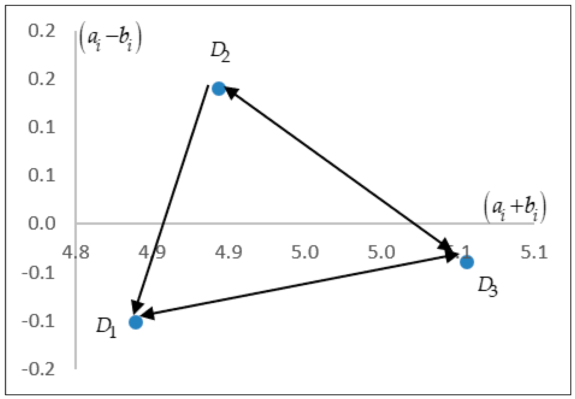
The NRM is constructed by mapping deneutrosophied $\left(a_i+b_i\right)$ and $\left(a_i-b_i\right)$ values. Figure 2 shows the coordinates of the dimensions where $D_1$ is influenced by $D_2$ and $D_3$. The threshold value is set at 0.33, which will produce the NRM among the dimensions, as shown in Figure 2.

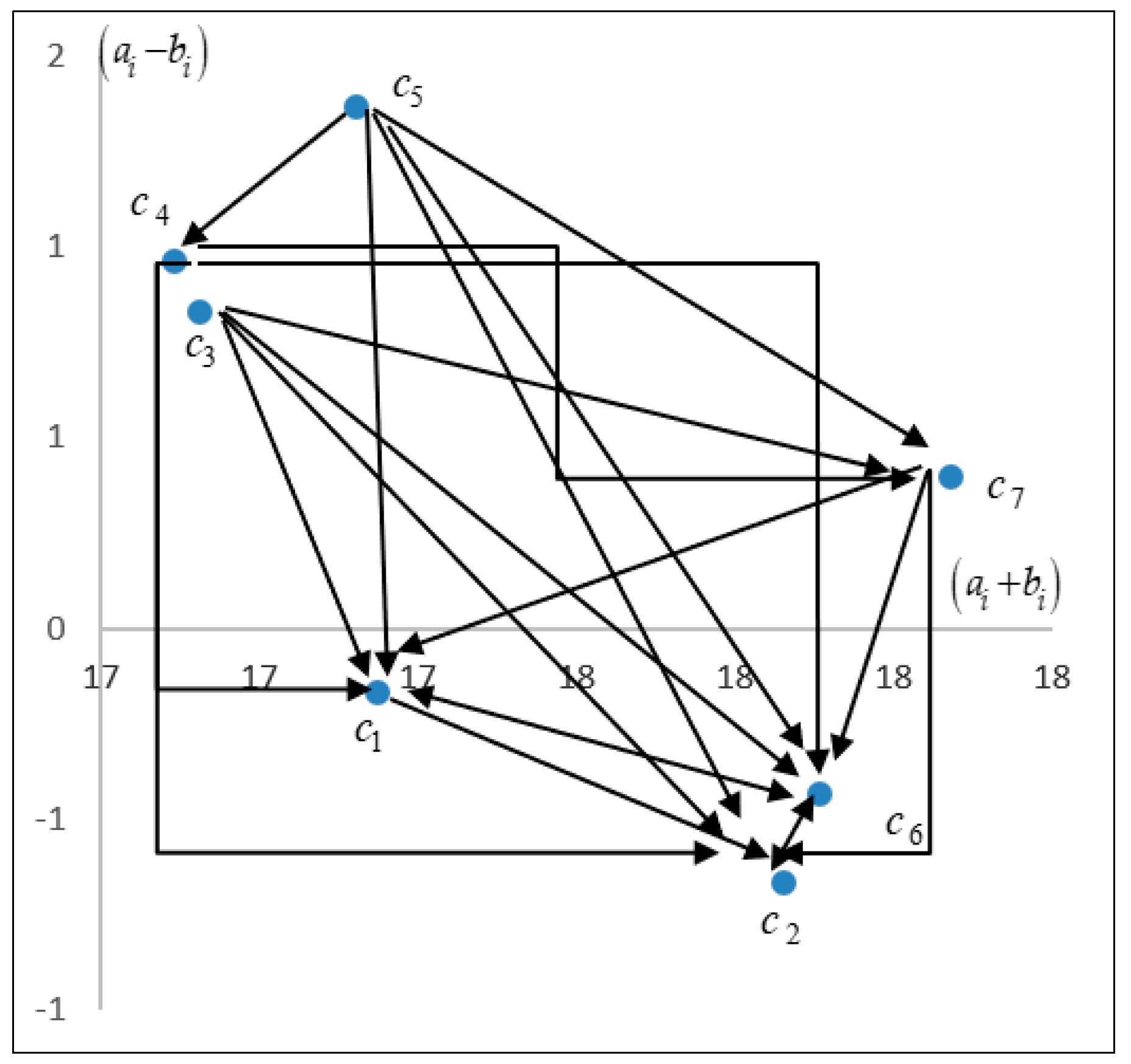
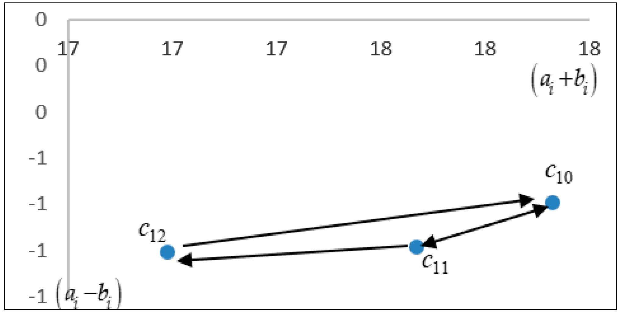
The threshold value for factors is set at 0.730. Thus, the coordinates and causal direction of the natural factors are presented after eliminating the minor effects and causes that were lower than the threshold value. Figure 3 shows the NRM of factors within dimension $D_1$.

For man-made factors of $D_2$ coastal erosion, the NRM is shown in Figure 4.

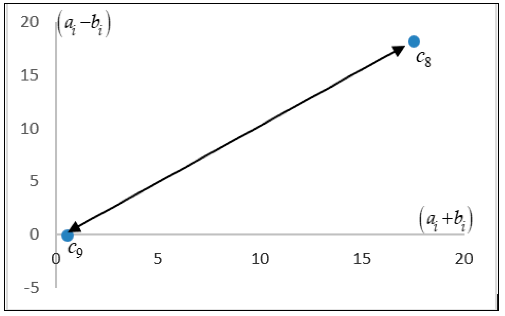
Under the socio-economic dimension, the factors are mapped in the negative quadrant of the $\left(a_i-b_i\right)$ axis. The coordinates of the three factors are shown in Figure 5.

The network relationship mapping obtained via the proposed method can provide a better understanding of the entire structure. Then, the neutrosophic total-influence matrix, S, is normalized using Equation (13), and it is shown in

Table 10. The new matrix $S_c^{\alpha }$.

	${\mathit{c}}_1$	${\mathit{c}}_2$	${\mathit{c}}_3$	${\mathit{c}}_4$	${\mathit{c}}_5$	${\mathit{c}}_6$	${\mathit{c}}_7$	${\mathit{c}}_8$	${\mathit{c}}_9$	${\mathit{c}}_{10}$	${\mathit{c}}_{11}$	${\mathit{c}}_{12}$
$c_1$	0.137	0.156	0.138	0.137	0.131	0.155	0.147	0.481	0.519	0.336	0.336	0.328
$c_2$	0.146	0.145	0.134	0.135	0.135	0.155	0.149	0.479	0.521	0.336	0.336	0.328
$c_3$	0.147	0.155	0.128	0.135	0.133	0.154	0.148	0.480	0.520	0.338	0.333	0.329
$c_4$	0.146	0.154	0.139	0.127	0.131	0.154	0.149	0.484	0.516	0.336	0.335	0.328
$c_5$	0.147	0.154	0.138	0.136	0.124	0.152	0.149	0.479	0.521	0.336	0.336	0.328
$c_6$	0.148	0.156	0.135	0.137	0.134	0.143	0.147	0.487	0.513	0.338	0.335	0.327
$c_7$	0.147	0.154	0.138	0.136	0.135	0.153	0.137	0.482	0.518	0.337	0.335	0.328
$c_8$	0.143	0.154	0.136	0.133	0.134	0.153	0.146	0.466	0.534	0.335	0.337	0.328
$c_9$	0.146	0.154	0.136	0.133	0.132	0.152	0.147	0.502	0.498	0.337	0.336	0.327
$c_{10}$	0.146	0.154	0.133	0.134	0.133	0.152	0.147	0.478	0.522	0.323	0.348	0.329
$c_{11}$	0.146	0.154	0.135	0.132	0.133	0.151	0.148	0.484	0.516	0.344	0.318	0.338
$c_{12}$	0.145	0.157	0.133	0.132	0.133	0.153	0.148	0.486	0.514	0.346	0.344	0.310

.

The next step is to construct the transpose matrix. By transposing the normalized neutrosophic total-influence matrix $S^{\alpha }$, the unweighted supermatrix $\psi$ is obtained.

Table 11. The unweighted supermatrix, $\psi$.

	${\mathit{c}}_1$	${\mathit{c}}_2$	${\mathit{c}}_3$	${\mathit{c}}_4$	${\mathit{c}}_5$	${\mathit{c}}_6$	${\mathit{c}}_7$	${\mathit{c}}_8$	${\mathit{c}}_9$	${\mathit{c}}_{10}$	${\mathit{c}}_{11}$	${\mathit{c}}_{12}$
$c_1$	0.137	0.146	0.147	0.146	0.147	0.148	0.147	0.143	0.146	0.146	0.146	0.145
$c_2$	0.156	0.145	0.155	0.154	0.154	0.156	0.154	0.154	0.154	0.154	0.154	0.157
$c_3$	0.138	0.134	0.128	0.139	0.138	0.135	0.138	0.136	0.136	0.133	0.135	0.133
$c_4$	0.137	0.135	0.135	0.127	0.136	0.137	0.136	0.133	0.133	0.134	0.132	0.132
$c_5$	0.131	0.135	0.133	0.131	0.124	0.134	0.135	0.134	0.132	0.133	0.133	0.133
$c_6$	0.155	0.155	0.154	0.154	0.152	0.143	0.153	0.153	0.152	0.152	0.151	0.153
$c_7$	0.147	0.149	0.148	0.149	0.149	0.147	0.137	0.146	0.147	0.147	0.148	0.148
$c_8$	0.481	0.479	0.480	0.484	0.479	0.487	0.482	0.466	0.502	0.478	0.484	0.486
$c_9$	0.519	0.521	0.520	0.516	0.521	0.513	0.518	0.534	0.498	0.522	0.516	0.514
$c_{10}$	0.336	0.336	0.338	0.336	0.336	0.338	0.337	0.335	0.337	0.323	0.344	0.346
$c_{11}$	0.336	0.336	0.333	0.335	0.336	0.335	0.335	0.337	0.336	0.348	0.318	0.344
$c_{12}$	0.328	0.328	0.329	0.328	0.328	0.327	0.328	0.328	0.327	0.329	0.338	0.310

shows the unweighted supermatrix.

Table 12. The new matrix $S_D^{\alpha }$.

	${\mathit{D}}_1$	${\mathit{D}}_2$	${\mathit{D}}_3$
$D_1$	0.29	0.36	0.35
$D_2$	0.35	0.27	0.38
$D_3$	0.36	0.36	0.28

shows the unweighted matrix of DMs.

By multiplying the elements in the unweighted supermatrix $\psi$ of factors (Table 11) and the new matrix of dimensions, $S_D^{\alpha }$ (Table 12), the weighted supermatrix, ${\psi }^{\alpha }$ in

Table 13. The weighted supermatrix ${\psi }^{\alpha }$ of dimensions.

	${\mathit{c}}_1$	${\mathit{c}}_2$	${\mathit{c}}_3$	${\mathit{c}}_4$	${\mathit{c}}_5$	${\mathit{c}}_6$	${\mathit{c}}_7$	${\mathit{c}}_8$	${\mathit{c}}_9$	${\mathit{c}}_{10}$	${\mathit{c}}_{11}$	${\mathit{c}}_{12}$
$c_1$	0.041	0.044	0.044	0.044	0.044	0.044	0.044	0.052	0.053	0.051	0.051	0.051
$c_2$	0.047	0.043	0.046	0.046	0.046	0.047	0.046	0.055	0.055	0.054	0.054	0.055
$c_3$	0.041	0.040	0.038	0.042	0.041	0.041	0.041	0.049	0.049	0.046	0.047	0.046
$c_4$	0.041	0.040	0.041	0.038	0.041	0.041	0.041	0.048	0.048	0.047	0.046	0.046
$c_5$	0.039	0.041	0.040	0.039	0.037	0.040	0.041	0.048	0.048	0.047	0.046	0.047
$c_6$	0.046	0.047	0.046	0.046	0.046	0.043	0.046	0.055	0.055	0.053	0.053	0.053
$c_7$	0.044	0.045	0.044	0.045	0.045	0.044	0.041	0.053	0.053	0.052	0.052	0.052
$c_8$	0.159	0.158	0.158	0.160	0.158	0.161	0.159	0.121	0.131	0.172	0.174	0.175
$c_9$	0.171	0.172	0.172	0.170	0.172	0.169	0.171	0.139	0.129	0.188	0.186	0.185
$c_{10}$	0.124	0.124	0.125	0.124	0.124	0.125	0.125	0.127	0.128	0.094	0.100	0.100
$c_{11}$	0.124	0.124	0.123	0.124	0.124	0.124	0.124	0.128	0.128	0.101	0.092	0.100
$c_{12}$	0.121	0.121	0.122	0.121	0.121	0.121	0.121	0.125	0.124	0.095	0.098	0.090

is constructed.

Table 14. The limiting supermatrix.

	c1	c2	c3	c4	c5	c6	c7	c8	c9	c10	c11	c12
c1	0.049	0.049	0.049	0.049	0.049	0.049	0.049	0.049	0.049	0.049	0.049	0.049
c2	0.052	0.052	0.052	0.052	0.052	0.052	0.052	0.052	0.052	0.052	0.052	0.052
c3	0.045	0.045	0.045	0.045	0.045	0.045	0.045	0.045	0.045	0.045	0.045	0.045
c4	0.045	0.045	0.045	0.045	0.045	0.045	0.045	0.045	0.045	0.045	0.045	0.045
c5	0.045	0.045	0.045	0.045	0.045	0.045	0.045	0.045	0.045	0.045	0.045	0.045
c6	0.051	0.051	0.051	0.051	0.051	0.051	0.051	0.051	0.051	0.051	0.051	0.051
c7	0.050	0.049	0.049	0.049	0.049	0.050	0.050	0.050	0.050	0.050	0.049	0.050
c8	0.153	0.153	0.153	0.153	0.153	0.153	0.153	0.153	0.153	0.153	0.153	0.153
c9	0.164	0.164	0.164	0.164	0.164	0.164	0.164	0.164	0.164	0.164	0.164	0.164
c10	0.116	0.116	0.116	0.116	0.116	0.116	0.116	0.116	0.116	0.116	0.116	0.116
c11	0.116	0.116	0.116	0.116	0.116	0.116	0.116	0.116	0.116	0.116	0.116	0.116
c12	0.113	0.113	0.113	0.113	0.113	0.113	0.113	0.113	0.113	0.113	0.113	0.113

shows the limited supermatrix by limiting the power of the weighted supermatrix.

Finally, the rows in the limited supermatrix contribute the weight of the factor of coastal erosion. The overall local weights and global weights of factors and dimensions are illustrated in

Table 15. The weights of dimensions and factors of coastal erosion.

Dimensions/Factors	Local Weights	Global Weights
Natural factors	0.336
Wave and current (c1)	0.145	0.049
Sediment transport (c2)	0.153	0.052
Storm surge (c3)	0.136	0.045
Tidal range (c4)	0.135	0.045
Global warming (c5)	0.132	0.045
Beach profile and stability (c6)	0.152	0.051
Sea level rise (c7)	0.146	0.05
Man-made factors	0.317
Sand mining activities (c8)	0.484	0.153
Coastal development (c9)	0.516	0.164
Socio-economic factors	0.347
Coastal protection (c10)	0.338	0.116
Budgetary revenue (c11)	0.337	0.116
Coastal zone management (c12)	0.326	0.113

.

The results show that coastal development (C₉) is the most important factor, with a weight of 0.164, followed by sand mining activities (C₈) at 0.153 and coastal protection (C₁₀) and budgetary revenue (C₁₁), which are both at 0.116. Relative to other factors, the DM suggests that the storm surge (C₃), tidal range (C₄), and global warming (C₅) are the least important factors with the global weights of 0.045. With respect to each dimension, the DMs indicate that sediment transport (C₂) is the most important factor in the dimension of natural factors (D₁), while coastal development (C₉) is the most important of the man-made factors (D₂). It also concludes that coastal protection (C₁₀) and budgetary revenue (C₁₁) are the most important factors under socio-economic factors (D₃).

4.5. Discussion and Implications

Based on the results, we know that the degrees of influence of coastal erosion factors are different from each other. The traditional average method, which assumes that the weights of clusters are equal, is thus irrational. Therefore, the normalized total-influence matrix S_c of DEMATEL is incorporated into the ANP method, which is able to consider the influential weight of each cluster. The findings show that the coastal development with the weightage of 0.164 is the most important factor for coastal erosion. Consequently, this study clearly shows the influence of the man-made factors on coastal erosion. Man-made factors such as coastal development are one of the factors that influenced the coastal environment and triggered the destruction of the natural dynamic ecosystem and coastline changes. Human influence on coastal environment and erosion can be connected to the demands and effects of coastal development. The development along coastal areas includes the engineering works such as land reclamation for urban expansion and airport extension, the dredging of navigational channels, and the construction of ports, harbors, groynes, breakwaters, and jetties. These developments can cause the interruption of long-shore sediment supply, which can cause either coastal erosion or accretion. Therefore, the government or stakeholders should pay more attention to the development projects near the coastal zone areas.

In addition, the problems of coastal erosion can be improved based on the NRM in Figure 2, Figure 3, Figure 4 and Figure 5, which were obtained via the DEMATEL method to comprehensively understand the interrelationships between dimensions and factors. Through the NRM, (a_i + b_i) indicates the degree of influences given and received, and it shows the importance index that each dimension and factor contributed to the problem. On the other hand, (a_i − b_i) categorizes the factors into net causer and net receiver groups. If the (a_i − b_i) value is positive, it indicates that the particular factor is influenced by the other factors, and if (a_i − b_i) is negative, then it means that the factor is being influenced by other factors. Considering the (a_i + b_i) and (a_i − b_i) values in Figure 2, it seems that the man-made factor should first be improved, because it influences the other dimensions the most. That is, if stakeholders plan the man-made factor well, it will improve the other two dimensions. They also can begin on the coastal development factor and sand-mining activities to improve the man-made factors dimension. As seen in Figure 2, it also determines that the natural factors dimension is being influenced the most, followed by the socio-economic factors dimension.

Collectively, this study of combining neutrosophic DEMATEL and ANP methods provides a comprehensive yet simple decision-making model, which can help solve complicated decision problems. This study outlines a critical role for finding the importance of each dimension and provides important insights on how to improve the coastal erosion problems.

5. Comparative Analysis

The comparative analysis is also made to compare the degree of importance of criteria obtained using the proposed method with the DEMATEL, fuzzy DEMATEL, and neutrosophic DEMATEL methods.

Table 16. The results of coastal erosion study using different methods.

Evaluation Method	Degree of Importance	Type of Number Used
DEMATEL	c9 > c10 > c7 > c2 > c6 > c11 > c8 > c1 > c3 > c12 > c5 > c4	Real number
Fuzzy DEMATEL	c9 > c7 > c10 > c2 > c6 > c11 > c8 > c1 > c3 > c5 > c12 > c4	Triangular fuzzy number
Neutrosophic DEMATEL	c9 > c7 > c10 > c6 > c2 > c11 > c8 > c1 > c5 > c12 > c3 > c4	Single Valued Neutrosophic Number
NS-DANP	c9 > c7 > c10 > c6 > c2 > c11 > c8 > c1 > c5 > c12 > c3 > c4	Single Valued Neutrosophic Number

shows a comparative analysis of the proposed NS-DANP method with the DEMATEL, fuzzy DEMATEL, and neutrosophic DEMATEL methods, and the respective type of number used.

Based on the Table 16, the degree of importance of factors obtained using the DEMATEL method, fuzzy DEMATEL method, neutrosophic DEMATEL method, and our proposed NS-DANP method are almost consistent. It also can be seen that the results of the neutrosophic DEMATEL method and our proposed NS-DANP method are exactly the same. However, the DEMATEL method only produces the end result of the degree of importance, while our proposed integrated ANP method with DEMATEL can give us the weights of every influential factor. In addition to that, ANP can consider the interaction and dependencies that exist among factors and dimensions. The introduction of the SVNWA aggregation operator in the process of combining all the DMs’ judgments can be considered better than just the normal averaging operator. Another distinct feature of the proposed method is the application of SVNSs into the proposed method, which makes it superior to the real number and triangular fuzzy numbers. The SVNS has an edge in dealing with a problem that is characterized by not only uncertainty but also truth, indeterminacy, and falsity information.

6. Conclusions

In this paper, an integrated ANP and DEMATEL method under the neutrosophic environment has been successfully developed. The neutrosophic DEMATEL-based ANP (NS-DANP) method offers two main contributions. Firstly, the single-valued neutrosophic numbers (SVNNs) are used instead of crisps or triangular fuzzy numbers (TFNs) to cater to the indeterminacy elements in the decision-making problem. The linguistic evaluation scale from Biswas et al. [65] was employed to obtain a comprehensive judgment. Secondly, we used the single-valued neutrosophic weighted averaging (SVNWA) aggregation operator proposed by Ye [66] to aggregate all the DMs’ judgments. This aggregation operator is simple but powerful enough to aggregate the SVNSs without losing the information.

A case study of the coastal erosion along Peninsular Malaysia coastline areas with 12 factors was implemented using the proposed NS-DANP method to get the most important factor. The results reveal that coastal development is the most important factor, followed by sand mining activities, coastal protection, and budgetary revenue. The stakeholders should pay extra attention to these three factors to minimize the coastal erosion events. The proposed method also successfully classified the factors of coastal erosion into two groups. The factors that caused the coastal erosion problem are sea level rise, tidal range, storm surge, global warming, and sand-mining activities. The other group of factors is known as the effects group, which includes sediment transport, waves and currents, coastal development, beach profile and stability, coastal protection, budgetary revenue, and coastal zone management.

A comparative analysis on the ranking of coastal erosion factors between the proposed NS-DANP method and the other existing methods was done. The results show that the proposed NS-DANP method is consistent with the neutrosophic DEMATEL method and almost consistent with the other two methods. Thus, we can conclude that the proposed NS-DANP is comparable with the other methods. Overall, the proposed NS-DANP method highlights the criteria weight and development of the causal diagram by applying single-valued neutrosophic numbers and the concept of the SVNWA aggregation operator. Besides that, the flaws in computing the multiplicative inverse of fuzzy matrices can be avoided, as SVNNs were used. Nonetheless, this study has some limitations. The relationships between the ideal number of DMs and reliability of the output have been a big question mark in the decision-making field. However, there are several mathematical methods that could be used in validating the reliability of the results. One of them is the sensitivity analysis, which can be incorporated in the future. The analysis could be used to check the sensitivity of the findings in the NRM due to a variety of uncertainty sources in linguistic evaluation.

References

1. Hsu, C.; Kuo, T.; Chen, S. Using DEMATEL to develop a carbon management model of supplier selection in green supply chain management. J. Clean. Prod. 2013, 56, 164–172. [Google Scholar] [CrossRef]
2. Lee, W.; Yihou, A.; Chang, Y. Analysis of decision making factors for equity investment by DEMATEL and Analytic Network Process. Expert Syst. Appl. 2011, 38, 8375–8383. [Google Scholar] [CrossRef]
3. Al-Faifi, A.; Song, B.; Hassan, M.M.; Alamri, A.; Gumaei, A. A hybrid multi criteria decision method for cloud service selection from Smart data. Future Gener. Comput. Syst. 2019, 93, 43–57. [Google Scholar] [CrossRef]
4. Mavi, R.K.; Standing, C. Cause and effect analysis of business intelligence (BI) benefits with fuzzy DEMATEL. Knowl. Manag. Res. Pract. 2018, 16, 245–257. [Google Scholar] [CrossRef]
5. Bahadori, M.; Ravangard, R.; Nezhad, M.T. Designing an interactive model of factors affecting the health technology assessment (HTA) in Iran. Int. J. Health Gov. 2018, 23, 301–311. [Google Scholar]
6. Yadegaridehkordi, E.; Hourmand, M.; Nilashi, M. Influence of big data adoption on manufacturing companies’ performance: An integrated DEMATEL-ANFIS approach. Technol. Forecast. Soc. Chang. 2018, 137, 199–210. [Google Scholar] [CrossRef]
7. Chirra, S.; Kumar, D. Evaluation of Supply Chain Flexibility in Automobile Industry with Fuzzy DEMATEL Approach. Glob. J. Flex. Syst. Manag. 2018, 19, 305–319. [Google Scholar] [CrossRef]
8. Ramezankhani, M.J.; Torabi, S.A.; Vahidi, F. Supply chain performance measurement and evaluation: A mixed sustainability and resilience approach. Comput. Ind. Eng. 2018, 126, 531–548. [Google Scholar] [CrossRef]
9. Awang, A.; Ghani, A.T.A.; Abdullah, L. The Shapley weighting vector-based neutrosophic aggregation operator in DEMATEL method. J. Phys. Conf. Ser. 2018, 1132, 012059. [Google Scholar] [CrossRef]
10. Li, Y.; Mathiyazhagan, K. Application of DEMATEL approach to identify the influential indicators towards sustainable supply chain adoption in the auto components manufacturing sector. J. Clean. Prod. 2016, 172, 2931–2941. [Google Scholar] [CrossRef]
11. Rad, T.G.; Sadeghi-Niaraki, A.; Abbasi, A. A methodological framework for assessment of ubiquitous cities using ANP and DEMATEL methods. Sustain. Cities Soc. 2018, 37, 608–618. [Google Scholar]
12. Saaty, T.L. The Analytic Hierarchy Process; McGraw-Hill: New York, NY, USA, 1980. [Google Scholar]
13. Shyur, H.J. COTS evaluation using modified TOPSIS and ANP. Appl. Math. Comput. 2006, 177, 251–259. [Google Scholar] [CrossRef]
14. Saaty, T.L. Decision Making with Dependence and Feedback: The Analytic Network Process; RWS Publications: Pittsburgh, PA, USA, 1996; p. 370. ISBN 0-9620317-9-8. [Google Scholar]
15. Daǧdeviren, M.; Yüksel, I. A fuzzy analytic network process (ANP) model for measurement of the sectoral competititon level (SCL). Expert Syst. Appl. 2010, 37, 1005–1014. [Google Scholar] [CrossRef]
16. Abdullah, L.; Zulkifli, N. Integration of fuzzy AHP and interval type-2 fuzzy DEMATEL: An application to human resource management. Expert Syst. Appl. 2015, 42, 4397–4409. [Google Scholar] [CrossRef]
17. Bhowmik, S.; Jagadish, G.K. Modeling and Optimization of Abrasive Water Jet Machining Process. In Modeling and Optimization of Advanced Manufacturing Processes; Springer: Cham, Switzerland, 2019; pp. 29–44. [Google Scholar]
18. Moktadir, M.A.; Ali, S.M.; Rajesh, R. Modeling the interrelationships among barriers to sustainable supply chain management in leather industry. J. Clean. Prod. 2018, 181, 631–651. [Google Scholar]
19. Ashtarinezhad, E.; Sarfaraz, A.H.; Navabakhsh, M. Supplier evaluation and categorize with combine Fuzzy Dematel and Fuzzy Inference System. Data Brief 2018, 18, 1149–1156. [Google Scholar] [CrossRef] [PubMed]
20. Chakraborty, S.; Chatterjee, P.; Prasad, K. An Integrated DEMATEL–VIKOR Method-Based Approach for Cotton Fibre Selection and Evaluation. J. Inst. Eng. Ser. E 2018, 99, 63–73. [Google Scholar] [CrossRef]
21. Cedolin, M.; Sener, Z. A fuzzy group decision making approach for supplier evaluation and selection in textile industry. In Uncertainty Modelling in Knowledge Engineering and Decision Making, Proceedings of the 12th International FLINS Conference, Roubaix, France, 24–26 August 2016; ENSAIT: Roubaix, France, 2016; pp. 794–799. [Google Scholar]
22. Tavana, M.; Khalili-Damghani, K.; Rahmatian, R. A hybrid fuzzy MCDM method for measuring the performance of publicly held pharmaceutical companies. Ann. Oper. Res. 2014, 226, 589–621. [Google Scholar] [CrossRef]
23. Adalı, E.A.; Işık, A.T. Integration of DEMATEL, ANP and DEA methods for third party logistics providers’ selection. Manag. Sci. Lett. 2016, 6, 325–340. [Google Scholar] [CrossRef]
24. Bongo, M.F.; Alimpangog, K.M.S.; Loar, J.F. An application of DEMATEL-ANP and PROMETHEE II approach for air traffic controllers’ workload stress problem: A case of Mactan Civil Aviation Authority of the Philippines. J. Air Transp. Manag. 2018, 68, 198–213. [Google Scholar] [CrossRef]
25. Mihajlovi, M.; Pamučar, D.; Mihajlović, M. Novel approach to group multi-criteria decision making based on interval rough numbers: Hybrid DEMATEL-ANP-MAIRCA model. Expert Syst. Appl. 2017, 88, 58–80. [Google Scholar]
26. Fetanat, A.; Khorasaninejad, E. A novel hybrid MCDM approach for offshore wind farm site selection: A case study of Iran. Ocean Coast. Manag. 2015, 109, 17–28. [Google Scholar] [CrossRef]
27. Lu, M.T.; Lin, S.W.; Tzeng, G.H. Improving RFID adoption in Taiwan’s healthcare industry based on a DEMATEL technique with a hybrid MCDM model. Decis. Support Syst. 2013, 56, 259–269. [Google Scholar] [CrossRef]
28. Tzeng, G.; Huang, C. Combined DEMATEL technique with hybrid MCDM methods for creating the aspired intelligent global manufacturing & logistics systems. Ann. Oper. Res. 2012, 197, 159–190. [Google Scholar]
29. Ju, Y.; Wang, A.; You, T. Emergency alternative evaluation and selection based on ANP, DEMATEL, and TL-TOPSIS. Nat. Hazards 2015, 75, 347–379. [Google Scholar] [CrossRef]
30. Baykasoklu, A.; Golcuk, I. An analysis of DEMATEL approaches for criteria interaction handling within ANP. Expert Syst. Appl. 2016, 46, 346–366. [Google Scholar]
31. Zadeh, L.A. Fuzzy Sets. Inf. Control. 1965, 8, 338–353. [Google Scholar] [CrossRef]
32. Lin, K.P.; Tseng, M.L.; Pai, P.F. Sustainable supply chain management using approximate fuzzy DEMATEL method. Resour. Conserv. Recycl. 2018, 128, 134–142. [Google Scholar] [CrossRef]
33. Abdullah, L.; Zulkifli, N. A new DEMATEL method based on interval type-2 fuzzy sets for developing causal relationship of knowledge management criteria. Neural Comput. Appl. 2018, 1–17. [Google Scholar] [CrossRef]
34. Senturk, S.; Erginel, N.; Binici, Y. Interval type-2 fuzzy analytic network process for modelling a third-party logistics (3PL) company. J. Mult.-Valued Log. Soft Comput. 2017, 28, 311–333. [Google Scholar]
35. Ozdemir, A.; Tuysuz, F. An Integrated Fuzzy DEMATEL and Fuzzy ANP Based Balanced Scorecard Approach: Application in Turkish Higher Education Institutions. J. Mult.-Valued Log. Soft Comput. 2017, 28, 251–287. [Google Scholar]
36. Chen, J.K.; Chen, I.S. Using a novel conjunctive MCDM approach based on DEMATEL, fuzzy ANP, and TOPSIS as an innovation support system for Taiwanese higher education. Expert Syst. Appl. 2010, 37, 1981–1990. [Google Scholar] [CrossRef]
37. Mavi, K.R.; Standing, C. Critical success factors of sustainable project management in construction: A fuzzy DEMATEL-ANP approach. J. Clean. Prod. 2018, 194, 751–765. [Google Scholar] [CrossRef]
38. George-Ufot, G.; Qu, Y.; Orji, I.J. Sustainable lifestyle factors influencing industries’ electric consumption patterns using Fuzzy logic and DEMATEL: The Nigerian perspective. J. Clean. Prod. 2017, 162, 624–634. [Google Scholar] [CrossRef]
39. Gan, J.; Luo, L. Using DEMATEL and Intuitionistic Fuzzy Sets to Identify Critical Factors Influencing the Recycling Rate of End-Of-Life Vehicles in China. Sustainability 2017, 9, 1873. [Google Scholar] [CrossRef]
40. Pandey, A.; Kumar, A. Commentary on “Evaluating the criteria for human resource for science and technology (HRST) based on an integrated fuzzy AHP and fuzzy DEMATEL approach”. Appl. Soft Comput. J. 2017, 51, 351–352. [Google Scholar] [CrossRef]
41. Seker, S.; Zavadskas, E.K. Application of fuzzy DEMATEL method for analyzing occupational risks on construction sites. Sustainability 2017, 9, 2083. [Google Scholar] [CrossRef]
42. Alam-tabriz, A.; Rajabani, N.; Farrokh, M. An Integrated Fuzzy DEMATEL-ANP-TOPSIS Methodology for Supplier Selection Problem. Glob. J. Manag. Stud. Res. 2014, 1, 85–99. [Google Scholar]
43. Hiete, M.; Merz, M.; Comes, T. Trapezoidal fuzzy DEMATEL method to analyze and correct for relations between variables in a composite indicator for disaster resilience. OR Spectr. 2012, 34, 971–995. [Google Scholar] [CrossRef]
44. Hosseini, M.B.; Tarokh, M.J. Type-2 fuzzy set extension of DEMATEL method combined with perceptual computing for decision making. J. Ind. Eng. Int. 2013, 9, 1–10. [Google Scholar] [CrossRef]
45. Baykasoğlu, A.; Gölcük, İ.; Han, W. Development of an interval type-2 fuzzy sets based hierarchical MADM model by combining DEMATEL and TOPSIS. Expert Syst. Appl. 2017, 70, 37–51. [Google Scholar] [CrossRef]
46. Büyüközkan, G.; Güleryüz, S.; Karpak, B. A new combined IF-DEMATEL and IF-ANP approach for CRM partner evaluation. Int. J. Prod. Econ. 2017, 191, 194–206. [Google Scholar] [CrossRef]
47. Govindan, K.; Khodaverdi, R.; Vafadarnikjoo, A. Intuitionistic fuzzy based DEMATEL method for developing green practices and performances in a green supply chain. Expert Syst. Appl. 2015, 42, 7207–7220. [Google Scholar] [CrossRef]
48. Keshavarzfard, R.; Makui, A. An IF-DEMATEL-AHP based on Triangular Intuitionistic Fuzzy Numbers (TIFNs). Decis. Sci. Lett. 2015, 4, 237–246. [Google Scholar] [CrossRef]
49. Han, W.; Sun, Y.; Xie, H. Hesitant Fuzzy Linguistic Group DEMATEL Method with Multi-granular Evaluation Scales. Int. J. Fuzzy Syst. 2018, 20, 2187–2201. [Google Scholar] [CrossRef]
50. Asan, U.; Kadaifci, C.; Bozdag, E. A new approach to DEMATEL based on interval-valued hesitant fuzzy sets. Appl. Soft Comput. J. 2018, 66, 34–49. [Google Scholar] [CrossRef]
51. Wang, H.; Smarandache, F.; Zhang, Y. Single Valued Neutrosophic Sets. Multisp. Multistruc. 2010, 4, 410–413. [Google Scholar]
52. Atanassov, T. Intuitionistic Fuzzy Sets. Fuzzy Sets Syst. 1986, 20, 87–96. [Google Scholar] [CrossRef]
53. Atanassov, K.; Gargov, G. Interval valued intuitionistic fuzzy sets. Fuzzy Sets Syst. 1989, 31, 343–349. [Google Scholar] [CrossRef]
54. Smarandache, F.A. Unifying Field in Logics: Neutrosophic Logic. Neutrosophy: Neutrosophic Probability, Set and Logic; American Research Press: Rehoboth, DE, USA, 1999. [Google Scholar]
55. Ye, J. Clustering methods using distance-based similarity measures of single-valued neutrosophic sets. J. Intell. Syst. 2014, 23, 379–389. [Google Scholar] [CrossRef]
56. Peng, J.; Wang, J.; Wang, J. Simplified neutrosophic sets and their applications in multi-criteria group decision-making problems. Int. J. Syst. Sci. 2016, 47, 2342–2358. [Google Scholar] [CrossRef]
57. Liu, P.; Wang, Y. Multiple attribute decision-making method based on single-valued neutrosophic normalized weighted Bonferroni mean. Neural Comput. Appl. 2014, 25, 2001–2010. [Google Scholar] [CrossRef]
58. Şahin, R.; Kucuk, A. Subsethood measure for single valued neutrosophic sets. J. Intell. Fuzzy Syst. 2015, 29, 525–530. [Google Scholar] [CrossRef]
59. Pramanik, S.; Dalapati, S.; Roy, T.K. Logistics Center Location Selection Approach Based on Neutrosophic Multi-Criteria Decision Making. In New Trends in Neutrosophic Theory and Applications; Pons-Editions: Brussels, Belgium, 2016; pp. 161–174. [Google Scholar]
60. Mondal, K.; Pramanik, S. Multi-criteria Group Decision Making Approach for Teacher Recruitment in Higher Education under Simplified Neutrosophic Environment. Glob. J. Eng. Sci. Res. Manag. 2014, 6, 28–34. [Google Scholar]
61. Ye, J.; Fu, J. Multi-period medical diagnosis method using a single valued neutrosophic similarity measure based on tangent function. Comput. Methods Programs Biomed. 2016, 123, 142–149. [Google Scholar] [CrossRef] [PubMed]
62. Mao, X.B.; Wu, M.; Dong, J.Y. A new method for probabilistic linguistic multi-attribute group decision making: Application to the selection of financial technologies. Appl. Soft Comput. J. 2019, 77, 155–175. [Google Scholar] [CrossRef]
63. Zhao, N.; Xu, Z.; Ren, Z. Hesitant fuzzy linguistic prioritized superiority and inferiority ranking method and its application in sustainable energy technology evaluation. Inf. Sci. 2019, 478, 239–257. [Google Scholar] [CrossRef]
64. Hu, J.; Pan, L.; Yang, Y. A group medical diagnosis model based on intuitionistic fuzzy soft sets. Appl. Soft Comput. 2019, 77, 453–466. [Google Scholar] [CrossRef]
65. Biswas, P.; Pramanik, S.; Giri, B.C. TOPSIS method for multi-attribute group decision-making under single-valued neutrosophic environment. Neural Comput. Appl. 2016, 27, 727–737. [Google Scholar] [CrossRef]
66. Ye, J. A multicriteria decision-making method using aggregation operators for simplified neutrosophic sets. J. Intell. Fuzzy Syst. 2014, 26, 2459–2466. [Google Scholar]
67. Luo, S.; Wang, H.; Cai, F. An integrated risk assessment of coastal erosion based on fuzzy set theory along Fujian coast, southeast China. Ocean Coast. Manag. 2013, 84, 68–76. [Google Scholar] [CrossRef]
Figure 1. The framework of the proposed neutrosophic Decision Making Trial and Evaluation Laboratory (DEMATEL)-based Analytic Hierarchy Process (ANP) (NS-DANP) method.
Symmetry 11 00328 g001
Figure 2. The network relationship map (NRM) within dimensions of coastal erosion.
Symmetry 11 00328 g002
Figure 3. The NRM within factors of natural factors ( D 1 ) of coastal erosion.
Symmetry 11 00328 g003
Figure 4. The NRM within factors of man-made factors ( D 2 ) of coastal erosion.
Symmetry 11 00328 g004
Figure 5. The NRM within factors of socio-economic factors ( D 3 ) of coastal erosion.
Symmetry 11 00328 g005