Article

Self-Adaptive Deep Multiple Kernel Learning Based on Rademacher Complexity

School of Computer Science and Engineerin, Central South University, Changsha 410083, China
*
Authors to whom correspondence should be addressed.
Symmetry 2019, 11(3), 325; https://doi.org/10.3390/sym11030325
Submission received: 8 January 2019 / Revised: 11 February 2019 / Accepted: 26 February 2019 / Published: 5 March 2019

Abstract

:
The deep multiple kernel learning (DMKL) method has caused widespread concern due to its better results compared with shallow multiple kernel learning. However, existing DMKL methods, which have a fixed number of layers and fixed type of kernels, have poor ability to adapt to different data sets and are difficult to find suitable model parameters to improve the test accuracy. In this paper, we propose a self-adaptive deep multiple kernel learning (SA-DMKL) method. Our SA-DMKL method can adapt the model through optimizing the model parameters of each kernel function with a grid search method and change the numbers and types of kernel function in each layer according to the generalization bound that is evaluated with Rademacher chaos complexity. Experiments on the three datasets of University of California—Irvine (UCI) and image dataset Caltech 256 validate the effectiveness of the proposed method on three aspects.

1. Introduction

The success of the Support Vector Machine (SVM) [1] makes the kernel method attract more attention [2,3,4]. The kernel function can be used to lift the dimension of data, and different kernels can be used to promote different categories of data to high-dimensional space or even infinite dimensions. Furthermore, the kernel trick makes the linear machine learning problem easy to be generalized to the nonlinear one, which enables the learning method to operate in a high-dimensional, implicit feature space without computing the data in that high-dimensional space.
However, these single kernel methods are based on a single feature space. As different kernel functions have different characteristics, the performance of kernel functions varies greatly in different applications. There is no perfect theoretical basis for the construction or selection of kernel function. In order to solve these problems, a lot of multiple kernel learning (MKL) methods using kernel combinations were proposed [5,6,7]. Gönen et al. gave a taxonomy of multiple kernel learning algorithms and reviewed them in detail [8]. In many cases, the multiple kernel model does not improve the accuracy much more, and these combinations do not change the kernel structure; thus, how to choose a suitable kernel function is still a problem, just like single kernel learning methods.
Many researchers integrate deep learning concepts with kernel learning in order to improve learning performance. Deep learning methods transform the input data through multiple nonlinear processing layers to construct new features [9]. These methods successfully make a dramatic improvement in pattern recognition. However, these methods have been limited to data sets with a very large sample size. Deep multiple kernel learning (DMKL) aims to learn “deep” kernel machines by exploring combinations of multiple kernels in a multi-layer structure [10]. Through multilevel mapping, the proposed MLMKL (Multi-Layer Multiple Kernel Learning) framework provides more flexibility than conventional MKL to find the optimal kernel for the application. In [11], a back-propagation MLMKL framework is proposed with the idea of deep learning to learn the optimal combination of the kernels. Three deep kernel learning models for breast cancer classification problem are presented in [12] to avoid overfitting risk appeared in deep learning. However, these models do not have a high generalization ability.
In order to solve the above problems, a self-adaptive deep multiple kernel learning (SA-DMKL) method is proposed in this paper. Unlike tradition DMKL, the SA-DMKL model includes several different base kernels in each layer. We propose a model learning algorithm to adapt the model with changing the model parameters of each kernel function with grid search method and the numbers and types of kernel function in each layer according to the a generalization bound that is evaluated with Rademacher chaos complexity. Therefore, our model is not very sensitive to the initial parameter settings for each candidate kernel function and avoids the handcrafted kernel selection before the learning process. In addition, the learning method is used to select kernel functions according to the input sample set in each layer by calculating the generalization bound based on Rademacher chaos complexity for each kernel function of each layer, and the Rademacher chaos complexity is used to evaluate the ability of a kernel function to map one sample space to another sample space. In this way, the selected kernel combination in each layer can improve the generalization ability.
The main contributions of our methods are summarized as follows: (1) A self-adaptive deep multiple kernel learning architecture is proposed. This SA-DMKL architecture includes several different basic kernels in each layer and the layer grows along with the learning process. Our architecture is also not very sensitive to the initial parameter settings of each candidate kernel function. (2) An SA-DMKL model learning algorithm to adapt the architecture is designed. Our learning algorithm uses the generalization bound based on Rademacher chaos complexity to select the kernel function, including the numbers of the kernel function in each layer, and the types of the kernel function. It aims to improve the generalization ability. Moreover, the parameters of each kernel function in each layer are optimized by a grid search method independently. (3) Experiments on UCI datasets and Caltech-256 dataset show that our SA-DMKL method has powerful generalization ability. Our SA-DMKL method has the best accuracy compared with other multiple kernel learning methods and has more effective accuracy than the multilayer multiple kernel learning method on most UCI data sets. The experimental results on the Caltech-256 dataset show that our SA-DMKL method is adaptive to the complex data set, which has large sample sizes and high dimensions.
The remainder of this paper is organized as follows: Section 2 briefly discusses the related works on deep multiple kernel learning and Rademacher complexity. Then, the SA-DMKL method including the architecture and the model learning algorithm is presented in Section 3Section 4 shows the experimental results on UCI datasets and Caltech-256 dataset and analyzes the validation. Some conclusions and future work are presented in Section 5.

2. Background

2.1. Deep Multiple Kernel Learning

Deep multiple kernel learning [10,11,12,13,14] has been actively studied in recent years inspired by deep learning. This method explores the combinations of multiple kernels in a multilayer architecture and has succeeded in a variety of sample sizes. Therefore, DMKL can be used in many real-world situations.
Cho et al. developed a multilayer kernel machine (MKM) that mimicked the computation in large neural nets with a family of arc-cosine kernel functions [15]. These arc-cosine kernels were combined with the -fold composition in multiple layers. This was the first work which integrated deep learning concepts with kernel learning. However, the arc-cosine kernel does not easily admit the hyper-parameters beyond the first layer.
In order to minimize the requirements of the domain knowledge, Ref. [10] introduced tunable hyper-parameters with infinite base kernel learning. The proposed infinite two-layer MKL method achieved more impressive performance than other MKL methods. However, this method had trouble to optimize the network beyond two layers to further enhance the performance.
In [13], an adaptive span deep multiple kernel learning method was proposed to improve the previous methods. This method combined kernels at each layer and then optimized the multiple complete layers of kernels throughout the leav × 10 on × 10 out procedure over an estimate of the support vector machine. The experimental results showed that each layer successfully increased the performance with only a few base kernels. Unfortunately, the improvements were not obtained using 3-layer rather than 2-layer.
Rebai et al. proposed the back propagation algorithm with the gradient method to learn the optimal combination of the kernels instead of the leav × 10 out-one error [11]. This method was very simple from a computational perspective and successfully optimized the system over many layers.
In fact, the deep multiple kernel learning method has a good effect on the generalization ability when the candidate kernel function and parameters are adjusted to a very appropriate level. However, it is very difficult to achieve such an effect. There are many hyperparameters that need to be set and it is also very difficult to adjust. Meanwhile, the existing DMKL architectures are relatively simple. Each layer is composed of a group of the same basic kernel functions, and the output of the kernel function of the previous layer serves as the input of all the kernel functions of the next layer. Furthermore, the number of layers is fixed. The lack of the selection of kernel function, and the fixed layers of the architecture lead to insufficient adaptability to the sample data and affect the performance of the model.

2.2. Rademacher Complexity

Rademacher complexity obtained significant concern and widespread applications in generalization ability analysis [16]. Koltchinskii first introduced the Rademacher penalty to the structural risk minimization problem [17]. Rademacher complexity is data-dependent, which can attain more compact generalization representation than other data-independent complexities.
Ying and Campbell developed a generalization bound for learning the kernel problem with Rademacher chaos complexity [18]. The method showed that the suprema of the Rademacher chaos process of order 2 over a candidate kernel could be used to analyze the generalization of the kernel learning algorithms.
According to [18], the true error or generalization error ϵ ϕ is defined as Equation (1):
ϵ ϕ ( f ) = X × Y ϕ ( y . f ( x ) ) d ρ ( x , y ) ,
where ϕ : R [ 0 , ) is a loss function, ρ is an unknown distribution on Z = X × Y , f ( x ) is a function f : X R , y is the true label, and the target function is defined by f ρ ϕ = arg min θ ϵ ϕ ( f ) .
Let the empirical error ϵ Z ϕ be defined by Equation (2):
ϵ Z ϕ ( f ) = 1 n j N n ϕ ( y j × f ( x j ) ) ,
where N n = { 1 , 2 , 3 , , n } for any n N , and Z is a set of training samples { z i = ( x i , y i ) : x i X , y i Y } that are independently and identically distributed in a classification problem on the input space X R d and the output space Y = { 1 , 1 } .
Let ϕ be a normalized classifying loss. For any δ ( 0 , 1 ) , with probability at least 1 δ , the following inequation (3) holds [18]:
ϵ ϕ ( f Z ϕ ) ϵ Z ϕ ( f Z ϕ ) 2 C λ ϕ ( 2 R ^ n ( κ ) λ n ) + 2 κ C λ ϕ ( 1 n λ ) 1 2 + 3 M λ ϕ ( ln ( 2 δ ) n ) 1 2 ,
where λ is the coefficient of the regular term, C λ ϕ , M λ ϕ are a local Lipschitz constant. κ = s u p k K , x X k ( x , x ) , and K is a kernel function set defined in Section 3. R ^ n ( κ ) is the empirical Rademacher chaos complexity, and it is estimated by entropy integrals.
In order to prohibit the divergence of the entropy integrals, Lei and Ding introduced an adjustable parameter to attain the balance between the accuracy and the complexity [19]. Strobl and Visweswaran pointed out that multiple layers increased the richness of the kernel representation according to the upper bound of the Rademacher chaos complexity [13]. Many research results show that Rademacher chaos complexity is a powerful tool to measure the complexity of kernel functions. In this paper, Rademacher chaos complexity is used to calculate the generalization bound to select the kernel function among the different base kernel functions in deep multiple kernel learning to improve the generalization.

3. Self-Adaptive Deep Multiple Kernels Learning SA-DMKL

3.1. SA-DMKL Architecture

The choice of kernel functions is very important for the performance of the kernel learning algorithm. Multiple kernel learning tries to select the appropriate kernel function according to some criteria. However, the major problem is that there are too many parameters with the increasing of the kernel functions, and deep multiple kernel learning makes the situation worse. Moreover, the fixed architecture in DMKL cannot adapt to the complexity of the training data. This paper proposes a self-adaptive deep multiple kernel learning architecture to tackle this problem.
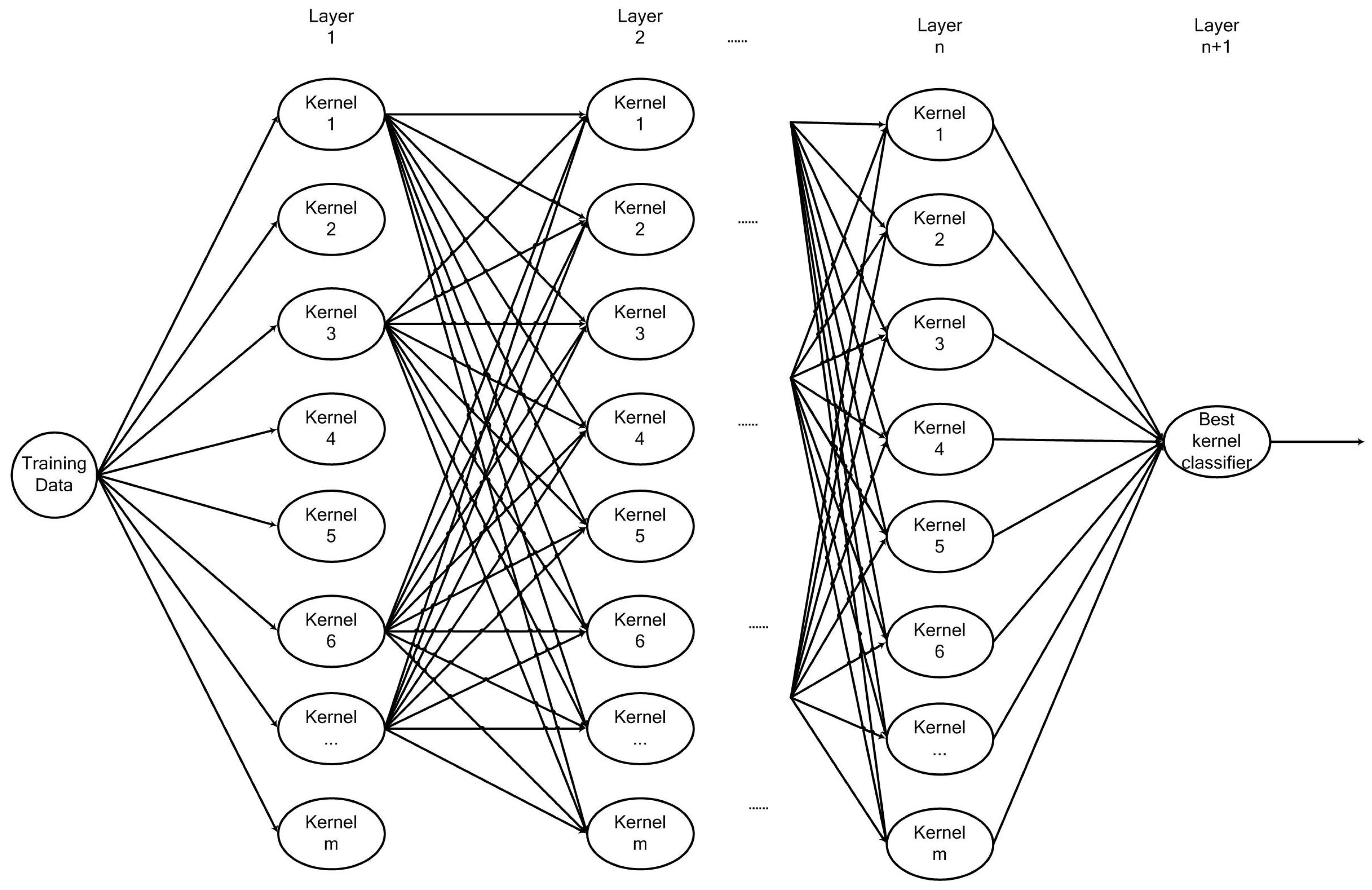
Our architecture is not very sensitive to the initial parameter settings of each candidate kernel function. In each layer, the parameters of each base candidate kernel function are optimized with the grid search method. The number of the layer is not fixed in SA-DMKL architecture. If the parameter settings are inappropriate, our model learning algorithm can adjust the architecture at the next layer. This means that SA-DMKL consists of multilayer multiple base kernel, as shown in Figure 1. In the first layer, the training data is used to separately train each candidate base kernel-based support vector machine (SVM), and the parameters of each base kernel will be adjusted by the grid search method. We evaluate each base kernel function using the generalization bound based on Rademacher chaos complexity and drop out the base kernels with larger generalization bound. The outputs of the rest kernel functions are used to construct a new feature space, and the dimension of this new feature space is the number of the rest kernel functions. For each training data, there is a corresponding new data in the new feature space. Those new data are input to the next layer to train each candidate base kernel with SVM. In the final layer, a kernel-based SVM is used to classify the training data.

3.2. Model Learning Algorithm

Given a set of training data D = { ( x i , y i ) | i = 1 , 2 , , n } , where x i X R d is the feature vector and y i { 1 , + 1 } is the class label. Our goal is to learn a deep multiple kernel network and a classifier f from the labeled training data. Here, f is an SVM based classifier.
Let K = { K l | κ l ( x i , x j ) = < ϕ l ( x i ) , ϕ l ( x j ) > ; l = 1 , 2 , , m ; i , j = 1 , 2 , , n } be a set of base candidate kernel functions, where ϕ is a feature map function. The Rademacher chaos complexity R ^ n ( k ) of k K is estimated according to the following rules:
  • If k is a Gaussian-type kernel, then
    R ^ n ( k ) ( 1 + 192 e ) κ 2 .
  • Otherwise,
    R ^ n ( k ) 25 e κ 2 lg ( m + 1 ) ,
where κ = s u p k K , x X k ( x , x ) , e is the base of the natural logarithm, and m is the number of elements of the base kernel function set K.
The generalization bound can be summarized from inequations (3) to (5). The local Lipschitz constant C λ ϕ , M λ ϕ is estimated according to Equations (6) and (7), where ϕ is the loss function, and λ  is the regularization parameter of a two-layer minimization problem:
C λ ϕ = s u p { ϕ ( x ) ϕ ( x ) | x x | : | x | , | x | κ 1 / λ } ,
M λ ϕ = s u p { | ϕ ( t ) | : | t | κ 1 / λ } .
In our model learning algorithm, the generalization bound is used to select the base kernel function. If the generalization bound is larger than the threshold, our algorithm will drop the corresponding base kernel out. This means that the dropout base kernel has poor generalization ability.
The learning performance of the SA-DMKL method is evaluated in terms of test accuracy according to Equation (8), which is the proportion of the correct classified samples to the total number of samples:
A c c u r a c y = T P + T N N ,
where TP is the number of true positive, TN is the number of true negatives, and N is the total number of instances in the test set.
In the model learning algorithm, the test accuracy is evaluated in each layer to decide whether the growth of the model ceases or not. If the test accuracy does not change in the fixed iterations, the iteration of the learning algorithm should be stopped.
The overall procedure of our model learning algorithm is described in Algorithm 1.
Algorithm 1 SA-DMKL algorithm.
Input:m: Number of candidate kernels;
  • k m : Initial parameters of each kernel function;
  • D: Dataset;
  • l: Maximum number of layers in which the best accuracy does not change;
  • R T : Threshold value of the generalization bound.

Output: Final model M.
1:
Initialize best accuracy A m = 0 ;
2:
Initialize maximum number of iteration i t e r ;
3:
Initialize current iteration i = 0 and flag j = 0 ;
4:
repeat
5:
    Randomly select 60 percent of samples from the entire dataset D as training samples D T ;
6:
    Use grid search method to adjust the initial parameters k m ;
7:
    Use D T to train m candidate kernel functions to create m SVMs;
8:
    Use m SVMs to predict the rest dataset D- D T and compute the test accuracy A t , generalization bound R t , and D t ; where t = 1 , 2 m ;
9:
    Initialize loop parameter l l = 1, and new dataset D p = ∅;
10:
    repeat
11:
        If R l l < R T then concatenate D p and D l l to generate new D p ;
12:
        If A l l A m then assign A l l to A m and assign 0 to j;
13:
         l l + + ;
14:
    until l l > m ;
15:
     If A m does not change then the flag j adds one;
16:
    Add one to i and assign D p to D;
17:
until ( i > = i t e r or j > = l )
According to Algorithm 1, each iteration from step 4 to step 17 builds one layer of the SA-DMKL architecture. In Algorithm 1, i stands for layer number, and j records the number of layers while A m remains the same. Step 5 to step 6 train m SVMs. In step 8, D t is calculated by tth kernel function with input data D, which is used in the next layer. In each iteration, the accuracy performance is evaluated for each support vector machine (SVM). If the best accuracy does not change in fixed iterations, the iteration should be stopped. Furthermore, the corresponding kernel of the SVM is discarded if its generalization bound is higher than the threshold value within step 10 to step 14.
4. Experiments and Results

4.1. Experimental Settings

In our experiments, we select five base kernel functions, and Table 1 shows their formulas and their initial parameter settings. RBF (Radial Basis Function), polynomial and arc-cosine kernels are commonly used kernel functions in the multilayer multiple kernel learning method. In Table 1, the parameter values are optimized with the grid search method in each iteration during the model learning process.
In order to simplify the experiments, the maximum number of iterations is initialized as 30, and the maximum number of layers l that best accuracy does not change is set as 4.

4.2. Datasets

4.2.1. UCI Data Sets

In order to evaluate the performance of our SA-DMKL method for classification tasks which have small size samples and dimensions, we choose seven data sets from the UCI database [20], which is described in Table 2.
We present an exhaustive comparative study using the following algorithms: SKSVM (SVM algorithm with a single RBF kernel), L2MKL [21], SM1MKL [22], DMKL [13], and MLMKL [11]. Table 3 shows the accuracy (%) results of the classification with those algorithms. Bold numbers indicate optimal results on a dataset.
Table 3 shows that our SA-DMKL method has more effective classification accuracy on most UCI data sets. Meanwhile, Table 3 indicates that multiple kernel learning has better classification accuracy than the single kernel learning, and deep multiple kernel learning can achieve more effective classification accuracy than the multiple kernel learning.

4.2.2. Caltech-256 Dataset

Caltech-256 is an image object recognition dataset, which contains 30,608 images and 256 object categories, with a minimum of 80 images and a maximum of 827 images per category [23]. We choose the Caltech-256 dataset to evaluate the performance of our SA-DMKL method for classification tasks that have large sample sizes and high dimensions.
In our experiment, we randomly select four categories of data: AK-47, baseball-bat, American flag, and a blimp. Some samples are shown in Figure 2.
In order to find out whether image preprocessing could affect the performance of SA-DMKL or not, we randomly select three image preprocessing methods, such as HoG (Histogram of Gradient), FFT (Fast Fourier Transformation), and simple image size changing. Figure 3 gives some image preprocessing examples.

4.3. Results and Analysis

4.3.1. Influence without Kernel Removing

In our model learning algorithm, we need to remove the kernel if its generalization bound value is larger than the threshold. In order to verify the influence without removing kernel, we set the threshold R T = + , and the experimental results are shown in Table 4 and Table 5. Here, A stands for classification accuracy on test data set, S stands for the number of the support vectors, and R stands for the corresponding generalization bound.
According to the results in Table 4 and Table 5, we conclude that, if we fix the type of the kernel in the multiple kernels learning, the learned model may not have the best test accuracy. It indicates that the traditional deep multiple kernel learning, which has a fixed number of layers and fixed type of kernels, may not be effective for finding the optimal learning model.

4.3.2. Influence of Different Types of Kernels

Table 6 and Table 7 show the experiment results, which are used to evaluate the influence of different kernels. We set the threshold R T = 10,000. This means that, if the value of R is greater than 10,000, which is marked by being underlined in the following tables, then the corresponding kernel should be removed at the corresponding layer.
Table 6 shows that the best classification accuracy is 0.92. Laplacian kernel and RBF kernel achieve the best classification accuracy at the 2nd and 3rd layers. Table 7 shows that the best classification accuracy is 0.97. RBF kernel is the only one kernel function which achieves the best classification accuracy. According to the experimental results, we find that the polynomial kernel is removed at each layer. The experiment results show that a different kernel has a different generalization bound at a different layer.
Table 6 and Table 7, compared with Table 4 and Table 5, respectively, show that removing the kernels, in which the generalization bound is larger than the threshold, improves the test accuracy.

4.3.3. Influence of Feature Extraction

In order to deal with the data set that has large sample sizes and high dimensions, feature extraction preprocessing is critical. We randomly choose three feature extraction methods, such as HoG, FFT, and resize methods, to evaluate the influence of different feature extraction methods. The experimental results are shown in Table 8, Table 9 and Table 10. The value of R, which is greater than the threshold, is marked by being underlined.
Compared with Table 4 to Table 7, we find that our SA-DMKL method needs many more layers to achieve the best classification accuracy. It means that complex data need a complex model. Our SA-DMKL method can construct an adequate model in accordance with the complexity of the training dataset.
According to the experimental results, the best classification accuracy is 0.82 or 0.83. The results show that our method can be adaptive to the image preprocessing. However, we find that the image preprocessing can affect the complexity of the model, such as the number of layers. For example, SA-DMKL obtains the best classification accuracy at the 3rd layer on Caltech 256 dataset with FFT feature extraction image preprocessing.

5. Conclusions

In this paper, a new multilayer multiple kernel learning method named SA-DMKL is proposed. The architecture of SA-DMKL is not fixed. It uses Rademacher chaos complexity to compute the generalization bound of the kernel function. SA-DMKL uses the generalization bound to select the kernel function in each layer. The model learning algorithm of SA-DMKL iteratively builds the model layer by layer. The experimental results show that the fixed architecture is not effective for DMKL, and our SA-DMKL method can adapt the model by itself through changing the model parameters of each kernel function, and the numbers and types of kernel function in each layer. In future work, we plan to integrate more learning techniques into our SA-DMKL method, such as model compression and model optimization, in order to realize our SA-DMKL method in an embedded system.

Author Contributions

S.R. conceived the idea; W.S. and S.R. designed the experiments; W.S. and Y.L. performed the experiments; W.S. and S.R. analyzed the data; S.R., W.S. and C.N.S. wrote the paper.

Funding

This research was funded by the Central South University Graduate Research Innovation Project Grant No. 2018zzts612.

Conflicts of Interest

The authors declare no conflict of interest.

References

  1. Vapnik, V.N. Statistical Learning Theory; Macmillan: New York, NY, USA, 1998. [Google Scholar]
  2. Muller, K.R.; Mika, S.; Ratsch, G.; Tsuda, K.; Scholkopf, B. An introduction to kernel based learning algorithms. IEEE Trans. Neural Netw. 2001, 12, 181–201. [Google Scholar] [CrossRef] [PubMed]
  3. Shaw-Taylorf, J.; Cristianini, N. Kernel Method for Pattern Analysis; Cambridge University Press: New York, NY, USA, 2004. [Google Scholar]
  4. Stock, M.; Pahikkala, T.; Airola, A.; De, B.; Waegeman, W. A comparative study of pairwise learning methods based on kernel ridge regression. Neural Comput. 2018, 30, 2245–2283. [Google Scholar] [CrossRef] [PubMed]
  5. Ghanty, P.; Paul, S.; Pal, N. NEUROSVM: An architecture to reduce the effect of the choice of kernel on the performance of SVM. J. Mach. Learn. Res. 2009, 10, 591–622. [Google Scholar]
  6. Hao, X.; Hoi, S. MKBoost: A framework of multiple kernel boosting. IEEE Trans. Knowl. Data Eng. 2013, 25, 1574–1586. [Google Scholar]
  7. Wang, Y.; Liu, X.; Dou, Y.; Qi, L.; Yao, L. Multiple kernel learning with hybrid kernel alignment maximization. Pattern Recognit. 2017, 70, 104–111. [Google Scholar] [CrossRef]
  8. Gönen, M.; Alpaydm, E. Multiple kernel learning algorithms. J. Mach. Learn. Res. 2011, 12, 2211–2268. [Google Scholar]
  9. Lecun, Y.; Bengio, Y.; Hinton, G. Deep learning. Nature 2015, 521, 436–444. [Google Scholar] [CrossRef] [PubMed]
  10. Zhuang, J.; Tsang, I.W.; Hoi, S. Two-layer multiple kernel learning. J. Mach. Learn. Res. 2011, 15, 909–917. [Google Scholar]
  11. Rebai, I.; Belayed, Y.; Mahdi, W. Deep multilayer multiple kernel learning. Neural Comput. Appl. 2016, 27, 2305–2314. [Google Scholar] [CrossRef]
  12. Rabha, O.; Hassan, Y.F.; Saleh, M.W. New deep kernel learning based models for image classification. Int. J. Adv. Comput. Sci. Appl. 2017, 8, 407–411. [Google Scholar]
  13. Strobl, E.; Visweswaran, S. Deep multiple kernel learning. In Proceedings of the 12th International Conference on Machine Learning and Applications, Miami, FL, USA, 4–7 December 2013; pp. 414–417. [Google Scholar]
  14. Jiu, M.; Sahbi, H. Nonlinear deep kernel learning for image annotation. IEEE Trans. Image Process. 2017, 26, 1820–1832. [Google Scholar] [CrossRef] [PubMed]
  15. Cho, Y.; Saul, L.K. Kernel methods for deep learning. Adv. Neural Inf. Process. Syst. 2009, 28, 342–350. [Google Scholar]
  16. Wu, X.; Zhang, J. Researches on Rademacher complexities in statistical learning theory: A survey. Acta Autom. Sin. 2017, 43, 20–39. [Google Scholar]
  17. Koltchinskii, V. Rademacher penalties and structural risk minimization. IEEE Trans. Inf. Theory 2011, 47, 1902–1914. [Google Scholar] [CrossRef]
  18. Ying, Y.; Campbell, C. Rademacher chaos complexities for learning the kernel problem. Neural Comput. 2010, 22, 2858–2886. [Google Scholar] [CrossRef] [PubMed]
  19. Lei, Y.; Ding, L. Refined rademacher chaos complexity bounds with applications to the multikernel learning problem. Neural Comput. 2014, 26, 739–760. [Google Scholar] [CrossRef] [PubMed]
  20. Dua, D.; Efi, K.T. UCI Machine Learning Repository. Available online: http://archive.ics.uci.edu/ml (accessed on 9 January 2019).
  21. Kloft, M.; Brefeld, U.; Sonnenburg, S.; Zien, A. lp-norm multiple kernel learning. J. Mach. Learn. Res. 2011, 12, 953–997. [Google Scholar]
  22. Xu, X.; Tsang, I.; Xu, D. Soft margin multiple kernel learning. IEEE Trans. Neural Netw. Learn. Syst. 2013, 24, 749–761. [Google Scholar] [PubMed]
  23. Griffin, G.; Holub, A.; Perona, P. Caltech-256 Object Category Dataset. Available online: https://authors.library.caltech.edu/7694/1/CNS-TR-2007-001.pdf (accessed on 9 January 2019).
Figure 1. SA-DMKL architecture.
Symmetry 11 00325 g001
Figure 2. Caltech-256 Dataset.
Symmetry 11 00325 g002
Figure 3. Image preprocessing.
Symmetry 11 00325 g003
Table 1. The candidate base kernel functions.
KernelFormulaParameters
Laplacian k ( x , y ) = e x p ( x y δ ) δ = 1.2
Tanh k ( x , y ) = t a n h ( α < x , y > + c ) α = 1.2
c = 2.1
RBF k ( x , y ) = e x p ( | | x y | | 2 2 δ 2 ) δ = 0.7
Arc-cosine [15] k n ( x , y ) = 1 π x n y n J n ( θ )
θ = c o s 1 ( < x , y > x y )
J n ( θ ) = ( 1 ) n ( sin ( θ ) ) 2 n + 1 ( 1 sin ( θ ) θ ) ( π θ sin ( θ ) )
a and b
are L 0 norm
n = 0
Polynomial k ( x , y ) = ( α < x , y > + c ) d α = 1.2
c = 2.1
d = 1
Table 2. The seven publicly available datasets from UCI.
Dataset#Dimensions#Samples
Iris4150
Liver6345
Breast10683
Sonar60208
Australia14690
German241000
Monk6432
Table 3. Classification results on the UCI datasets. Bold numbers indicate optimal results.
DatasetAlgorithms
SKSVML2MKLSM1MKLDMKLMLMKLSA-DMKL
Liver6.366 × 10 1 6.750 × 10 1 6.883 × 10 1 6.901 × 10 1 7.180 × 10 1 7.565 × 10 1
Breast9.425 × 10 1 9.618 × 10 1 9.636 × 10 1 9.659 × 10 1 9.721 × 10 1 9.192 × 10 1
Sonar5.029 × 10 1 8.451 × 10 1 8.500 × 10 1 8.394 × 10 1 8.384 × 10 1 8.942 × 10 1
Australia7.154 × 10 1 8.164 × 10 1 8.289 × 10 1 8.440 × 10 1 8.542 × 10 1 8.203 × 10 1
German7.018 × 10 1 6.998 × 10 1 7.014 × 10 1 7.202 × 10 1 7.506 × 10 1 7.850 × 10 1
Monk9.032 × 10 1 9.722 × 10 1 9.666 × 10 1 9.662 × 10 1 9.689 × 10 1 9.755 × 10 1
Table 4. The results of SA-DMKL on the breast dataset from UCI (without kernel removing). Bold numbers indicate optimal results.
LayersLaplacianTanhRBFAr_cosinePolynomial
ASRASRASRASRASR
18.60  × 10 1 3.41  × 10 2 2.00  × 10 2 3.70  × 10 1 2.20  × 10 1 4.75  × 10 1 8.60  × 10 1 3.41  × 10 2 3.00  × 10 2 6.20  × 10 1 1.00  × 10 0 4.29  × 10 5 9.10  × 10 1 6.00  × 10 0 3.20  × 10 4
28.60  × 10 1 3.41  × 10 2 1.00  × 10 2 6.20  × 10 1 1.00  × 10 0 4.70  × 10 13 8.60  × 10 1 3.41  × 10 2 4.00  × 10 2 8.70  × 10 1 8.00  × 10 0 9.01  × 10 9 8.80  × 10 1 7.00  × 10 0 1.20  × 10 11
38.60  × 10 1 3.41  × 10 2 3.00  × 10 2 3.30  × 10 1 3.00  × 10 0 4.80  × 10 13 8.60  × 10 1 3.41  × 10 2 6.00  × 10 2 8.80  × 10 1 4.00  × 10 0 3.90  × 10 21 8.80  × 10 1 2.00  × 10 0 1.20  × 10 18
48.60  × 10 1 3.41  × 10 2 4.00  × 10 2 5.30  × 10 1 2.80  × 10 1 4.46  × 10 1 8.60  × 10 1 3.41  × 10 2 4.00  × 10 2 6.20  × 10 1 1.00  × 10 0 2.33  × 10 6 6.20  × 10 1 2.90  × 10 1 2.33  × 10 6
58.60  × 10 1 3.41  × 10 2 2.00  × 10 2 6.20  × 10 1 1.00  × 10 0 4.70  × 10 13 8.60  × 10 1 3.41  × 10 2 1.00  × 10 2 6.20  × 10 1 1.00  × 10 0 2.33  × 10 6 6.20  × 10 1 1.00  × 10 0 2.33  × 10 6
Table 5. The results of SA-DMKL on the iris dataset from UCI (without kernel removing). Bold numbers indicate optimal results.
layersLaplacianTanhRBFAr_cosinePolynomial
ASRASRASRASRASR
19.40  × 10 1 1.10  × 10 1 2.20  × 10 1 3.30  × 10 1 1.00  × 10 0 9.30  × 10 13 8.80  × 10 1 1.80  × 10 1 3.98  × 10 1 3.30  × 10 1 1.00  × 10 0 1.69  × 10 2 3.30  × 10 1 1.00  × 10 0 1.62  × 10 5
28.60  × 10 1 9.00  × 10 1 5.00  × 10 1 3.30  × 10 1 1.00  × 10 0 9.30  × 10 13 8.60  × 10 1 9.00  × 10 1 2.20  × 10 1 3.30  × 10 1 1.00  × 10 0 5.64  × 10 6 3.30  × 10 1 1.00  × 10 0 5.64  × 10 6
38.60  × 10 1 8.90  × 10 1 2.60  × 10 0 3.30  × 10 1 1.00  × 10 0 9.30  × 10 13 8.60  × 10 1 9.00  × 10 1 1.01  × 10 0 3.30  × 10 1 1.00  × 10 0 5.64  × 10 6 3.30  × 10 1 1.00  × 10 0 5.64  × 10 6
48.60  × 10 1 9.00  × 10 1 8.70  × 10 1 3.30  × 10 1 1.00  × 10 0 9.30  × 10 13 8.60  × 10 1 9.00  × 10 1 8.70  × 10 1 3.30  × 10 1 1.00  × 10 0 5.64  × 10 6 3.30  × 10 1 1.00  × 10 0 5.64  × 10 6
53.50  × 10 1 3.40  × 10 1 2.99  × 10 2 3.30  × 10 1 1.00  × 10 0 9.30  × 10 13 0.00  × 10 0 1.00  × 10 0 nan0.00  × 10 0 1.00  × 10 0 nan3.30  × 10 1 1.00  × 10 0 5.64  × 10 6
Table 6. The results of SA-DMKL on the breast cancer dataset from UCI. Bold numbers indicate optimal results. The value of R, which is greater than the threshold, is marked by being underlined.
LayersLaplacianTanhRBFAr_cosinePolynomial
ASRASRASRASRASR
18.50  × 10 1 3.41  × 10 2 2.00  × 10 2 7.00  × 10 1 2.30  × 10 1 2.74  × 10 1 8.70  × 10 1 3.41  × 10 2 1.00  × 10 2 6.20  × 10 1 1.00  × 10 0 3.17  × 10 5 9.10  × 10 1 4.20  × 10 1 2.53  × 10 6
29.20  × 10 1 3.20  × 10 1 1.84  × 10 0 3.10  × 10 1 1.23  × 10 2 6.00  × 10 2 9.20  × 10 1 3.10  × 10 1 8.10  × 10 1 6.50  × 10 1 2.40  × 10 1 1.39  × 10 6 7.20  × 10 1 1.00  × 10 0 2.19  × 10 6
39.20  × 10 1 1.30  × 10 1 1.20  × 10 1 8.50  × 10 1 6.00  × 10 0 1.40  × 10 1 9.20  × 10 1 2.00  × 10 1 1.30  × 10 1 6.20  × 10 1 1.00  × 10 0 3.33  × 10 0 6.20  × 10 1 1.00  × 10 0 4.36  × 10 13
47.50  × 10 1 1.20  × 10 1 2.48  × 10 0 7.70  × 10 1 3.00  × 10 0 6.11  × 10 0 7.40  × 10 1 1.80  × 10 1 4.29  × 10 0 6.20  × 10 1 1.00  × 10 0 6.27  × 10 1 6.20  × 10 1 1.00  × 10 0 1.26  × 10 14
57.40  × 10 1 1.50  × 10 1 2.13  × 10 0 6.20  × 10 1 1.00  × 10 0 2.90  × 10 13 7.40  × 10 1 2.70  × 10 1 2.00  × 10 0 6.20  × 10 1 1.00  × 10 0 1.09  × 10 3 6.20  × 10 1 1.00  × 10 0 2.33  × 10 6
67.40  × 10 1 2.30  × 10 1 1.35  × 10 0 6.20  × 10 1 1.00  × 10 0 2.90  × 10 13 7.30  × 10 1 3.40  × 10 1 2.01  × 10 0 3.70  × 10 1 5.00  × 10 0 7.39  × 10 4 6.20  × 10 1 3.00  × 10 0 2.30  × 10 6
77.30  × 10 1 7.00  × 10 0 2.90  × 10 0 8.50  × 10 1 7.00  × 10 0 4.02  × 10 0 7.30  × 10 1 6.00  × 10 0 2.02  × 10 0 7.30  × 10 1 3.00  × 10 0 4.54  × 10 1 6.20  × 10 1 1.00  × 10 0 2.33  × 10 6
Table 7. The results of SA-DMKL on the iris dataset from UCI. Bold numbers indicate optimal results. The value of R, which is greater than the threshold, is marked by being underlined.
LayersLaplacianTanhRBFAr_cosinePolynomial
ASRASRASRASRASR
19.40  × 10 1 1.10  × 10 1 3.05  × 10 0 3.30  × 10 1 1.00  × 10 0 9.30  × 10 13 8.80  × 10 1 1.80  × 10 1 1.10  × 10 1 3.30  × 10 1 1.00  × 10 0 1.69  × 10 2 3.30  × 10 1 1.00  × 10 0 1.62  × 10 5
29.60  × 10 1 7.60  × 10 1 3.09  × 10 0 3.30  × 10 1 1.00  × 10 0 9.30  × 10 13 9.50  × 10 1 7.80  × 10 1 6.10  × 10 1 3.30  × 10 1 1.00  × 10 0 5.40  × 10 5 3.30  × 10 1 1.00  × 10 0 5.64  × 10 6
39.50  × 10 1 6.00  × 10 0 2.99  × 10 2 8.70  × 10 1 2.00  × 10 0 9.30  × 10 1 9.70  × 10 1 8.00  × 10 0 2.99  × 10 2 9.40  × 10 1 3.00  × 10 0 3.12  × 10 1 3.30  × 10 1 1.00  × 10 0 9.10  × 10 14
49.30  × 10 1 6.00  × 10 0 2.99  × 10 2 8.90  × 10 1 4.00  × 10 0 1.53  × 10 0 9.30  × 10 1 6.00  × 10 0 2.99  × 10 2 3.30  × 10 1 1.00  × 10 0 2.43  × 10 4 3.30  × 10 1 1.00  × 10 0 5.64  × 10 6
59.20  × 10 1 1.00  × 10 1 1.12  × 10 0 3.30  × 10 1 1.00  × 10 0 9.30  × 10 13 0.90  × 10 0 1.10  × 10 1 2.63  × 10 0 3.30  × 10 1 1.00  × 10 0 4.53  × 10 3 3.30  × 10 1 1.00  × 10 0 8.01  × 10 5
68.90  × 10 1 4.10  × 10 1 3.41  × 10 0 3.30  × 10 1 1.00  × 10 0 9.30  × 10 13 8.70  × 10 1 3.80  × 10 1 3.39  × 10 0 3.30  × 10 1 1.00  × 10 0 1.42  × 10 6 3.30  × 10 1 1.00  × 10 0 5.64  × 10 6
78.70  × 10 1 7.00   × 10 0 2.41   × 10 0 8.30  × 10 1 2.00  × 10 0 4.25  × 10 0 8.70  × 10 1 7.00  × 10 0 2.39  × 10 0 8.70  × 10 1 5.00  × 10 0 1.75  × 10 2 3.30  × 10 1 1.00  × 10 0 5.64  × 10 6
Table 8. The results of SA-DMKL on the Caltech 256 dataset with the HoG method. Bold numbers indicate optimal results. The value of R, which is greater than the threshold, is marked by being underlined.
layersLaplacianTanhRBFAr_cosinePolynomial
ASRASRASRASRASR
14.00  × 10 1 1.10  × 10 1 2.65  × 10 1 5.70  × 10 1 1.00  × 10 0 5.58  × 10 1 4.10  × 10 1 2.30  × 10 1 1.81  × 10 0 5.20  × 10 1 2.70  × 10 1 4.24  × 10 0 5.70  × 10 1 1.00  × 10 0 5.53  × 10 6
24.70  × 10 1 5.6  × 10 1 6.00  × 10 2 5.70  × 10 1 5.00  × 10 0 6.30  × 10 15 6.10  × 10 1 6.00  × 10 1 1.00  × 10 2 5.90  × 10 1 1.80  × 10 1 2.15  × 10 2 5.90  × 10 1 9.00  × 10 0 1.47  × 10 7
36.20  × 10 1 3.80  × 10 1 1.20  × 10 1 6.35  × 10 1 1.00  × 10 1 2.19  × 10 0 6.50  × 10 1 4.40  × 10 1 5.00  × 10 2 6.70  × 10 1 4.10  × 10 1 1.32  × 10 7 5.70  × 10 1 1.00  × 10 0 4.63  × 10 6
46.30  × 10 1 2.60  × 10 1 6.00  × 10 2 4.10  × 10 1 2.00  × 10 1 5.21  × 10 1 7.20  × 10 1 2.20  × 10 1 1.00  × 10 2 5.90  × 10 1 9.00  × 10 0 3.40  × 10 1 6.00  × 10 1 1.40  × 10 1 1.12  × 10 1
56.00  × 10 1 7.90  × 10 1 6.00  × 10 2 6.20  × 10 1 3.10  × 10 1 5.67  × 10 1 5.70  × 10 1 8.00  × 10 0 4.60  × 10 15 5.90  × 10 1 8.00  × 10 0 1.05  × 10 6 5.70  × 10 1 1.00  × 10 0 1.41  × 10 10
67.40  × 10 1 2.30  × 10 1 2.1  × 10 1 5.50  × 10 1 1.70  × 10 1 2.80  × 10 0 7.20  × 10 1 1.90  × 10 1 3.90  × 10 1 5.70  × 10 1 1.00  × 10 0 2.64  × 10 0 5.70  × 10 1 1.00  × 10 0 2.20  × 10 3
77.50  × 10 1 6.00  × 10 1 1.10  × 10 1 5.70  × 10 1 1.00  × 10 0 5.58  × 10 13 7.40  × 10 1 4.50  × 10 1 5.00  × 10 2 5.70  × 10 1 1.00  × 10 0 1.97  × 10 4 5.70  × 10 1 1.00  × 10 0 5.83  × 10 5
87.70  × 10 1 3.30  × 10 1 6.00  × 10 2 7.40  × 10 1 5.00  × 10 0 2.00  × 10 2 7.80  × 10 1 2.60  × 10 1 1.00  × 10 2 7.50  × 10 1 3.00  × 10 1 3.51  × 10 2 5.70  × 10 1 1.00  × 10 0 5.60  × 10 0
98.00  × 10 1 7.60  × 10 1 2.00  × 10 2 5.00  × 10 1 1.00  × 10 0 5.58  × 10 13 8.00  × 10 1 7.60  × 10 1 1.34  × 10 1 5.70  × 10 1 1.00  × 10 0 2.86  × 10 3 5.70  × 10 1 1.00  × 10 0 2.96  × 10 5
108.20  × 10 1 8.70  × 10 1 2.00  × 10 2 5.70  × 10 1 1.00  × 10 0 5.58  × 10 13 8.20  × 10 1 8.70  × 10 1 5.2  × 10 2 5.70  × 10 1 1.00  × 10 0 4.63  × 10 6 5.70  × 10 1 1.00  × 10 0 4.63  × 10 6
118.20  × 10 1 2.00  × 10 0 3.00  × 10 2 8.20  × 10 1 3.00  × 10 0 5.58  × 10 13 8.20  × 10 1 3.00  × 10 0 6.00  × 10 2 8.10  × 10 1 3.00  × 10 0 1.49  × 10 2 5.70  × 10 1 1.00  × 10 0 1.63  × 10 3
128.00  × 10 1 2.00  × 10 0 3.87  × 10 2 5.70  × 10 1 1.00  × 10 0 5.58  × 10 13 8.00  × 10 1 2.00  × 10 0 3.37  × 10 1 5.70  × 10 1 1.00  × 10 0 1.45  × 10 3 5.70  × 10 1 1.00  × 10 0 1.78  × 10 8
138.00  × 10 1 2.00  × 10 0 3.87  × 10 1 5.70  × 10 1 1.00  × 10 0 5.58  × 10 13 7.90  × 10 1 2.00  × 10 0 1.00  × 10 2 5.70  × 10 1 1.00  × 10 0 9.07  × 10 6 5.70  × 10 1 1.00  × 10 0 4.77  × 10 4
148.00  × 10 1 2.00  × 10 0 3.87  × 10 1 2.00  × 10 1 1.00  × 10 0 5.58  × 10 13 7.90  × 10 1 2.00  × 10 0 9.40  × 10 1 5.70  × 10 1 1.00  × 10 0 4.85  × 10 3 5.70  × 10 1 1.00  × 10 0 5.18  × 10 2
Table 9. The results of SA-DMKL on the Caltech 256 dataset with the FFT method. Bold numbers indicate optimal results. The value of R, which is greater than the threshold, is marked by being underlined.
LayersLaplacianTanhRBFAr_cosinePolynomial
ASRASRASRASRASR
14.60  × 10 1 5.50  × 10 1 4.10  × 10 1 5.70  × 10 1 1.00  × 10 0 5.58  × 10 1 5.80  × 10 1 6.20  × 10 1 1.08  × 10 1 5.70  × 10 1 1.00  × 10 0 4.63  × 10 6 5.75  × 10 1 1.00  × 10 0 6.83  × 10 2
28.10  × 10 1 9.30  × 10 1 7.00  × 10 2 5.70  × 10 1 1.00  × 10 0 5.58  × 10 13 8.10  × 10 1 9.30  × 10 1 2.00  × 10 2 5.80  × 10 1 3.20  × 10 1 1.79  × 10 5 4.80  × 10 1 2.90  × 10 1 3.91  × 10 4
38.20  × 10 1 3.00  × 10 0 5.00  × 10 2 8.10  × 10 1 2.00  × 10 0 5.58  × 10 1 8.30  × 10 1 2.00  × 10 0 8.00  × 10 2 7.80  × 10 1 3.00  × 10 0 1.49  × 10 2 8.10  × 10 1 1.00  × 10 0 1.40  × 10 2
47.80  × 10 1 3.00  × 10 0 3.87  × 10 13 8.10  × 10 1 1.00  × 10 0 3.80  × 10 0 7.80  × 10 1 2.00  × 10 0 3.87  × 10 13 5.70  × 10 1 1.00  × 10 0 7.44  × 10 2 7.90  × 10 1 1.00  × 10 0 2.548  × 10 3
58.10  × 10 1 7.90  × 10 1 1.00  × 10 2 5.30  × 10 1 3.00  × 10 0 5.58  × 10 13 8.10  × 10 1 8.30  × 10 1 5.00  × 10 2 5.70  × 10 1 1.00  × 10 0 3.80  × 10 3 4.30  × 10 1 3.00  × 10 0 1.48  × 10 5
67.90  × 10 1 9.00  × 10 0 3.87  × 10 1 8.20  × 10 1 4.00  × 10 0 9.00  × 10 2 7.90  × 10 1 1.20  × 10 1 1.50  × 10 1 7.80  × 10 1 5.00  × 10 0 1.04  × 10 1 8.10  × 10 1 1.00  × 10 0 1.12  × 10 2
77.90  × 10 1 1.50  × 10 1 3.87  × 10 1 8.10  × 10 1 1.00  × 10 0 5.15  × 10 1 7.70  × 10 1 1.10  × 10 1 6.88  × 10 0 5.70  × 10 1 1.00  × 10 0 8.21  × 10 2 8.10  × 10 1 1.00  × 10 0 6.92  × 10 2
88.10  × 10 1 4.40  × 10 1 7.40  × 10 1 8.10  × 10 1 1.00  × 10 0 5.58  × 10 13 8.10  × 10 1 4.80  × 10 1 1.10  × 10 1 5.70  × 10 1 1.00  × 10 0 7.76  × 10 4 8.10  × 10 1 1.00  × 10 0 1.05  × 10 5
98.10  × 10 1 7.00  × 10 0 4.00  × 10 2 7.50  × 10 1 4.00  × 10 0 4.20  × 10 1 8.10  × 10 1 8.00  × 10 0 2.90  × 10 1 7.90  × 10 1 4.00   × 10 0 2.60  × 10 1 8.10  × 10 1 1.00  × 10 0 2.02  × 10 0
107.70  × 10 1 1.80  × 10 1 6.40  × 10 1 8.10  × 10 1 3.00  × 10 0 1.86  × 10 1 7.70  × 10 1 1.60  × 10 1 4.00  × 10 2 5.70  × 10 1 1.00  × 10 0 1.06  × 10 3 8.10  × 10 1 1.00  × 10 0 7.93  × 10 2
Table 10. The results of SA-DMKL on the Caltech 256 dataset without feature extraction. Bold numbers indicate optimal results. The value of R, which is greater than the threshold, is marked by being underlined.
LayersLaplacianTanhRBFAr_cosinePolynomial
ASRASRASRASRASR
16.20  × 10 1 5.60  × 10 1 2.00  × 10 2 5.90  × 10 1 6.00  × 10 0 1.22  × 10 1 4.20  × 10 1 4.40  × 10 1 2.88  × 10 0 5.7  × 10 1 1.00  × 10 0 4.63  × 10 6 5.70  × 10 1 1.00  × 10 0 3.54  × 10 6
27.80  × 10 1 7.30  × 10 1 5.00  × 10 2 4.30  × 10 1 8.00  × 10 0 1.30  × 10 8 5.20  × 10 1 7.20  × 10 1 5.00  × 10 2 5.70  × 10 1 1.00  × 10 0 5.79  × 10 1 5.70  × 10 1 1.00  × 10 0 2.57  × 10 4
35.80  × 10 1 7.50  × 10 1 1.00  × 10 2 5.70  × 10 1 1.00  × 10 0 5.58  × 10 13 5.90  × 10 1 7.10  × 10 1 7.00  × 10 2 5.70  × 10 1 1.00  × 10 0 8.15  × 10 5 5.70  × 10 1 1.00  × 10 0 4.63  × 10 6
46.70  × 10 1 2.10  × 10 1 1.00  × 10 2 5.90  × 10 1 3.00  × 10 0 7.08  × 10 0 6.60  × 10 1 2.10  × 10 1 7.00  × 10 2 5.70  × 10 1 1.00  × 10 0 4.22  × 10 0 5.70  × 10 1 1.00  × 10 0 3.64  × 10 0
58.20  × 10 1 8.60  × 10 1 1.9  × 10 1 5.70  × 10 1 1.00  × 10 0 5.58  × 10 13 8.20  × 10 1 8.70  × 10 1 7.00  × 10 2 5.70  × 10 1 1.00  × 10 0 4.08  × 10 5 5.70  × 10 1 1.00  × 10 0 4.63  × 10 6
68.20  × 10 1 4.00  × 10 0 1.98  × 10 1 8.20  × 10 1 4.00  × 10 0 5.57  × 10 1 8.20  × 10 1 4.00  × 10 0 3.83  × 10 1 7.60  × 10 1 2.00  × 10 0 1.01  × 10 2 5.70  × 10 1 1.00  × 10 0 9.42  × 10 2
78.20  × 10 1 6.00  × 10 0 1.60  × 10 1 8.20  × 10 1 6.00  × 10 0 5.58  × 10 1 8.20  × 10 1 6.00  × 10 0 2.30  × 10 1 5.70  × 10 1 1.00  × 10 0 5.75  × 10 2 5.70  × 10 1 1.00  × 10 0 2.61  × 10 3
88.20  × 10 1 1.20  × 10 1 3.70  × 10 1 8.20  × 10 1 8.00  × 10 0 1.20  × 10 1 8.20  × 10 1 1.20  × 10 1 3.87  × 10 1 5.70  × 10 1 1.00  × 10 0 6.00  × 10 1 5.70  × 10 1 1.00  × 10 0 1.16  × 10 3
98.20  × 10 1 5.10  × 10 1 8.00  × 10 2 5.70  × 10 1 1.00  × 10 0 5.57  × 10 13 8.20  × 10 1 6.00  × 10 1 1.00  × 10 2 5.70  × 10 1 1.00  × 10 0 1.96  × 10 3 5.70  × 10 1 1.00  × 10 0 4.63  × 10 6