Global Image Thresholding Adaptive Neuro-Fuzzy Inference System Trained with Fuzzy Inclusion and Entropy Measures

Abstract

Thresholding algorithms segment an image into two parts (foreground and background) by producing a binary version of our initial input. It is a complex procedure (due to the distinctive characteristics of each image) which often constitutes the initial step of other image processing or computer vision applications. Global techniques calculate a single threshold for the whole image while local techniques calculate a different threshold for each pixel based on specific attributes of its local area. In some of our previous work, we introduced some specific fuzzy inclusion and entropy measures which we efficiently managed to use on both global and local thresholding. The general method which we presented was an open and adaptable procedure, it was free of sensitivity or bias parameters and it involved image classification, mathematical functions, a fuzzy symmetrical triangular number and some criteria of choosing between two possible thresholds. Here, we continue this research and try to avoid all these by automatically connecting our measures with the wanted threshold using some Artificial Neural Network (ANN). Using an ANN in image segmentation is not uncommon especially in the domain of medical images. However, our proposition involves the use of an Adaptive Neuro-Fuzzy Inference System (ANFIS) which means that all we need is a proper database. It is a simple and immediate method which could provide researchers with an alternative approach to the thresholding problem considering that they probably have at their disposal some appropriate and specialized data.

1. Introduction

Thresholding is used in separating the foreground (which contains one or more objects) from the background of an image. This is achieved by rendering all of its pixels as either black or white. The result is a binarized version of our initial input which is usually the introductory step of other applications concerning image processing or computer vision. It is an important process and, though it may seem an easy task, it is in fact a complicated and elaborate procedure because of the wide variety of characteristics which are unique to each image. Thresholding techniques are sorted into two distinct groups: global thresholding methods and local or adaptive thresholding methods. The former assign a unique threshold to the whole image while the latter find a different threshold for every pixel based on the grayscale information of its adjoining pixels. Sometimes, these two are combined to some hybrid method. Local techniques are of course slower and they are usually used in cases where our input is degraded or contains multiple objects, lighting “irregularities” and various distortions. In samples like these, the performance of global methods is usually poor and their results are insufficient. However, in other cases, global techniques are preferred due to their speed and simplicity.

As far as global methods are concerned, when a specific intensity value between 0 and 255 (for greyscale images) is chosen as the threshold t of the image, the pixels whose intensity is larger than t are set as “white” while the other pixels are set as “black”. Depending on the way this value t is calculated, global techniques are categorized as histogram-shaped-based, clustering-based, entropy-based, object attribute-based and spatial approaches [1]. Although there are several general methods of image binarization, the quality of their results may vary depending on the set of images they are being applied on. In other words, some method may perform well for specific images but this doesn’t mean that it will be suitable for all inputs. Hence, we often need to confine our area of experimentation to specific domains of particular attributes.

In [2], we introduced some possible fuzzy inclusion measures and their respective (based on Young’s theorem [3]) fuzzy entropy measures. These measures were extracted from a specific formula in which we used fuzzy binary operations (fuzzy intersections or t-norms and fuzzy implications). At the same time, we tried to “enclose” these inclusion functions in some theoretical mathematical context by examining their possibility to follow some axioms concerning fuzzy subsethood. We saw that they can be connected with Young’s axioms [3] of fuzzy inclusion which were introduced as a link and a continuation of Kosko’s respective research on fuzzy subsethood and entropy [4,5,6]. Although we had to slightly alter one of Young’s original axioms, we didn’t invalidate the rest of her work (concerning the connection between fuzzy subsethood and fuzzy entropy as stated earlier by Kosko) which means that our inclusion measures returned some respective entropy measures according to her theorem.

Fuzzy subsethood and entropy functions can be used in a variety of applications (image processing, feature selection, fuzzy classification, fuzzy controllers, fuzzy rules, similarity measures) and there are several presentations dealing with such measures (e.g., [7,8,9,10,11,12,13,14,15,16,17,18,19], to name a few after 2000). In [2], while examining the behavior of our measures, we saw that some of them had some interesting attributes which could offer additional information when specific applications are concerned. In an attempt to prove the applicability of these measures as well as to support our belief that they could offer us a different approach to the solution of a particular problem, we also introduced a general algorithm of global image thresholding. This method efficiently used some of our indicators and was based entirely on them. This means that, unlike other methods of image thresholding, it does not rely on the histogram of the image nor does it depend on the optimization of some statistical or fuzzy measure. We didn’t involve with any kind of concavity or statistical analysis or fuzzy classification. We only used specific fuzzy inclusion values between the image and some standard images (black, white, grey). The entropy of the image was used as well. It is a very immediate and comprehensible method and its main characteristic is that it is an open and adaptable procedure which can be adjusted to the distinctive characteristics of someone’s area of interest.

Then, in [20,21], we adapted this general method to a local level. There, we focused on documents of non-uniform illumination and our algorithm was adjusted to cases of this particular domain. These text documents usually include text and line-drawings and there are several occasions where we need to recognize or improve their content. This can be achieved by their proper binarization and it is important for document analysis systems or optical character recognition (OCR) processes. Global methods are insufficient for this kind of images so we had to adjust our method to a local thresholding technique. Once again, the results were very competent while compared with those of MATLAB’s “adaptthresh” command (version: 9.0.0.341360-R2016a, The MathWorks Inc., Natick, MA, USA). It is also very important that we managed to present a fully automated procedure (regarding user provided constants) and we avoided sensitivity or bias parameters (which are used by most local methods) by properly exploiting some of the information that our measures provided.

After this research on a global and on a local level, we were convinced not only for the applicability of our measures but for their potential to offer valuable information to thresholding problems as well. Therefore, we thought that a next logical step to our research could be an effort of establishing the connection between our measures and desired threshold t in a automatic way. Based on our previous work, a fuzzy neural network seemed very appropriate for this task. One of our main goals here is to examine the possibility of using fuzzy inclusion and entropy measures as input variables of an inference system. Of course, the target setting of the whole process can be puzzling, but, at the same time, it may prove to be an advantage as well. For instance, it could help someone enhance specific results of an existing method (without having to modify or improve the method itself) or approach more specialized targets without having to fabricate a respective algorithm from scratch. Thus, our second goal is to support this argument by presenting some corresponding results. These derive from two specific systems trained with the ANFIS (Adaptive Neuro-Fuzzy Inference System) method. The first one tries to enhance specific binarizations of Otsu’s method on a particular set of images and the second one attempts to approach some more specialized results which are mainly focused on edge detection. These examples are only indicative and a visual expert could estimate this whole process better and more accurately.

After introduction, we have an overview on global thresholding methods and on adaptive neuro-fuzzy inference systems. We also summarize some basic parts of our previous work. In the next section, we explain the procedure that we followed and we present the results of our first global thresholding ANFIS which is trained with targets obtained from a combination of Otsu’s thresholds and human observation. Then, in Section 4, we experiment on public databases and we train a second ANFIS in order to achieve some more focused results which we evaluate both visually and numerically. This is followed by a summarization and some further discussion. Finally, Section 6 contains our conclusions.

2. ANFIS, Global Thresholding Techniques and the Main Parts of Our Previous Research

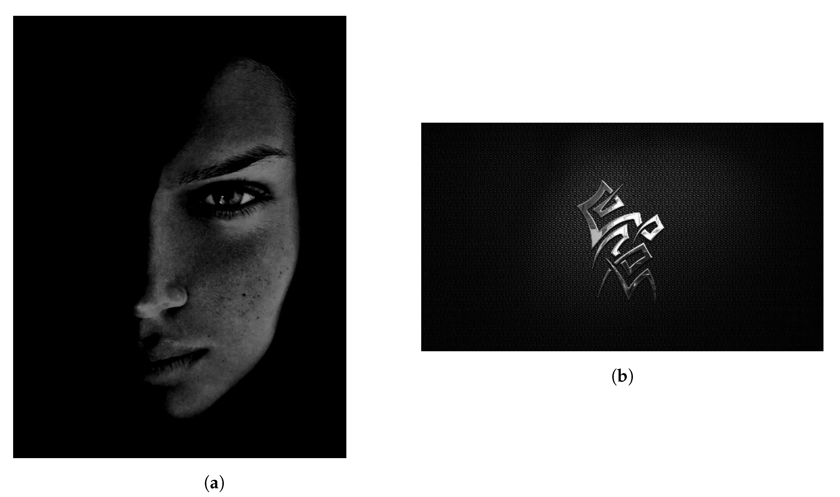
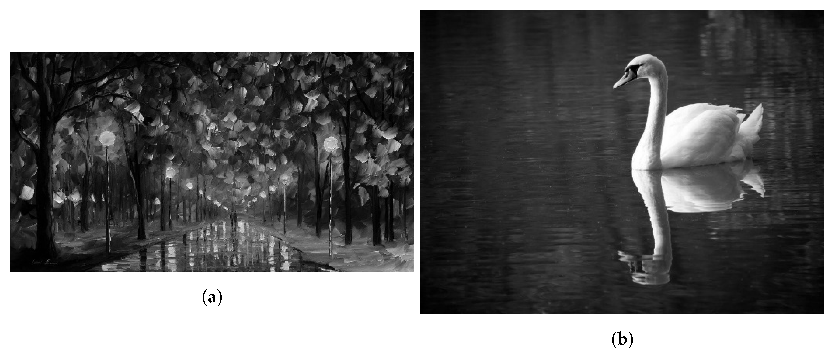
2.1. Global Thresholding Methods and Neural Networks in Image Segmentation

Like we said in our introduction, thresholding techniques are sorted (according to the information they obtain from the data) as histogram-shaped-based, clustering-based, entropy-based, object attribute-based, spatial approaches and local methods [1]. Histogram based methods analyze the shape properties of grey-level histograms. The proper threshold is estimated via concavity analysis or regularization and statistical measurements. Some methods examine the distance of the histogram from convex hull [22,23,24,25,26] and others use curvature analysis in order to find peaks and valleys or overlapping peaks [27,28,29]. In other cases, the histogram is converted into a smoothed two-peaked representation using auto-regressive modeling [30,31] or we have a rectangular approximation to the lobes of the histogram [32,33].

Clustering-based methods output two groups of pixels from gray-level information. Some iterative techniques search for the midpoints of the peaks [34,35,36,37], whereas other algorithms are based on minimization of the error between the form of the image and Gaussian distributions [38,39]. We also have techniques that use fuzzy clustering based on the histogram of the image [33,40] and methods relying on the optimization of some statistical measure. Otsu’s [41] method belongs in this category and it is one of the most referenced, well-known and widely used thresholding techniques ever.

Entropy-based methods exploit the entropy of the distribution of the gray levels of the image. The first who studied thresholding using Shannon’s entropy were Pal et al. [42] and Johannsen and Bille [43]. In some cases, we have an attempt of maximizing the entropy as an indication of maximum information transfer [44,45,46,47] and in others an effort of minimizing the entropy in order to have maximum information preservation [48,49,50,51].

Object attribute-based methods are based on some attribute quality or on the similarity between the original image and the binarized one. Such attributes may be edge matching [52], gray-level moments [53,54,55], shape compactness [56,57], connectivity [58], texture [59], or stability of segmented objects [60]. Other algorithms use fuzzy measures in order to calculate the resemblance between the original image and its binarized version [61,62].

Spatial methods use gray-level distribution along with the dependency of pixels in a local area. One of the first techniques was Rosenfeld’s [63] who used local average. We also have the use of relaxation [64,65], the Laplacian of the images [24], quadtrees [66] and second-order statistics [67]. Co-occurrence probabilities have also been used [68,69,70] as well as second-order entropy [71,72,73,74,75,76] and fuzzy partitioning [77,78]. There is also a method based on a posteriori spatial probability estimation [79] and one which uses the max-min distance to the extracted foreground object [80].

Of course, there are several variations or modifications of these algorithms as well. As someone can see, there are numerous presentations and a lot of different approaches dealing with thresholding; however, it still remains an open problem. Overall, the dependence of many methods on the shape of the histogram prevents them from generalization while other methods are bias or parameter dependent or have a significant computational cost. Generally, all thresholding techniques work well for some types of images but not for all of them. We also mentioned that local methods ([81,82,83,84] are some of the most known algorithms) calculate a different threshold for each pixel and we believe it is fair to be studied separately. In any case, here we focus on global thresholding fuzzy neural networks and we won’t elaborate on these techniques.

Finally, we need to mention that there are several attempts on image segmentation with the use of neural networks, especially in the case of medical images. According to Othman and Tizhoosh [85], methods with a self-organizing map (unsupervised learning) use a large number of parameters. Furthermore, these need to be modulated before training and their reliance on prior information complicates their generalization. In [86], we have a two-stage neural network for volume segmentation of medical images. The first stage consists of a self-organizing principal components analysis network and the second of a self-organizing map used for clustering. In [87], medical images are segmented using a constraint-based Hopfield network. An incremental neural network for the segmentation of tissues in ultrasound images is presented in [88] where discrete Fourier transform (DFT) and discrete cosine transform (DCT) are used. In [89], we have a constraint satisfaction neural network used on a survey on image segmentation and, in [90], we have self-organizing neural networks used in the segmentation of astronomical images.

What we present here is different from these methods and our technique directly derives from our algorithms in [2,20,21]. The binarization of the image is accomplished based solely on some fuzzy inclusion and entropy measurements (after our image is transformed into a fuzzy set) and we don’t use any information regarding the histogram of our input. Moreover, we don’t rely on any kind of analysis (concavity, statistical, etc.) of the image and no sensitivity or bias parameters are used. These inclusion and entropy values (five in total) constitute the inputs of our ANFIS while the target could be extracted—for example—from some other methods, human experience, data analysis or a combination of several procedures. All of these render our whole process very immediate and comprehensible and someone only needs some proper data to train his fuzzy system. Of course, the setting of the ground truth may be difficult or tiresome, nevertheless, it could help us improve specific results of a global technique or accomplish more specialized targets without having to modify the method itself or turning to more complex algorithms (local or hybrid).

2.2. Fuzzy Subsethood and Entropy Measures

In [2,91], we studied the production of possible fuzzy subsethood and entropy measures according to Young’s axioms and theorem. Let X be our universal set (a finite set), ⌀ its complement, $F\left(X\right)$ its power set and A, B members of X with corresponding membership grades $m_A\left(x\right)$ and $m_B\left(x\right)$. Moreover, $A^C$ will be the standard complement of A (meaning that $m_{A^C}\left(x\right)=1-m_A\left(x\right)$), P will be the fuzziest set ( $m_P\left(x\right)=1/2$ for every $x\in X$) and $A\subseteq B$ in Zadeh’s sense will mean that $m_A\left(x\right)\le m_B\left(x\right)$ for every $x\in X$. Next are Young’s original axiomatization of fuzzy inclusion and her theorem regarding fuzzy entropy measures:

Definition 1.

A fuzzy inclusion measure is a function $S:F\left(X\right)\times F\left(X\right)\to I$ which satisfies the following:

$S(A,B)=1$if and only if$A\subseteq B$in Zadeh’s sense,	(S1)
If$P\subseteq A$in Zadeh’s sense, then$S(A,A^c)=0\iff A=X$,	(S2)
If$B\subseteq A_1\subseteq A_2$, then$S(A_1,B)\ge$$S(A_2,B)$,	(S3)
and if$B_1\subseteq B_2$, then$S(A,B_1)\le S(A,B_2).$

Theorem 1.

If S is a fuzzy subsethood measure (meaning a function satisfying $S1$−$S3$), then E defined as

$$E\left(A\right)=S(A\cup A^c,A\cap A^c),A\in F\left(X\right)$$

is an entropy measure (according to De Luca and Termini, (1972)) of fuzzy set A, where

$$m_{A\cup A^c}\left(x\right)=max(m_A\left(x\right),1-m_A\left(x\right))\mathrm{and}{m}_{A\cap A^c}\left(x\right)=min(m_A\left(x\right),1-m_A\left(x\right)).$$

We initially tried to produce fuzzy inclusion measures (according to Young’s axioms) and their corresponding (according to Theorem 1) entropy measures based on the following formula:

$$S(A,B)=\left\{\begin{array}{cc}\frac{\underset{x\in X}{\sum T(}I(m_A\left(x\right),m_B\left(x\right)),m_A\left(x\right))}{{\displaystyle \sum _{x\in X}}{m}_A\left(x\right)}\hfill & \mathrm{if}A\ne ⌀,\hfill \\ 1\hfill & \mathrm{if}A=⌀,\end{array}\right.$$

(1)

where T is a fuzzy intersection (t-norm) and I is a fuzzy implication. Our incipient efforts to combine several known fuzzy t-norms and implications resulted in producing only Kosko’s measures [4,5,6]. After we replaced axiom $S3$ with the following:

If $P\subseteq A_1\subseteq A_2$, then $S(A_1,A_1^c)\ge$ $S(A_2,A_2^c)$	(S3${}^{\prime }$)
and if $B_1\subseteq B_2$, then $S(A,B_1)\le S(A,B_2)$

without affecting the rest of Young’s work, we managed to produce various possible fuzzy inclusion and entropy measures by combining several common fuzzy intersections and implications. More accurately, we had seven possible fuzzy inclusion indicators which satisfy—at least—$S1$, $S2$ and $S{3}^{\prime }$ and three corresponding entropy measures (some inclusion measures returned the same entropy indicators).

Here, once again, we focus on the following two inclusion indicators:

$$S_1(A,B)=\left\{\begin{array}{cc}\frac{{\displaystyle \sum _{x\in X}}{I}_Z(m_A\left(x\right),m_B\left(x\right))·m_A\left(x\right))}{{\displaystyle \sum _{x\in X}}{m}_A\left(x\right)}\hfill & \mathrm{if}A\ne ⌀,\hfill \\ 1\hfill & \mathrm{if}A=⌀,\hfill \end{array}\right.$$

(2)

and

$$S_2(A,B)=\left\{\begin{array}{cc}\frac{{\displaystyle \sum _{x\in X}}{I}_{Luc}(m_A\left(x\right),m_B\left(x\right))·m_A\left(x\right))}{{\displaystyle \sum _{x\in X}}{m}_A\left(x\right)}\hfill & \mathrm{if}A\ne ⌀,\hfill \\ 1\hfill & \mathrm{if}A=⌀,\hfill \end{array}\right.$$

(3)

where

$$I_Z(m_A\left(x\right),m_B\left(x\right))=\left\{\begin{array}{c}1\mathrm{if}{m}_A\left(x\right)\le m_B\left(x\right)\hfill \\ max(m_{A^c}\left(x\right),m_B\left(x\right))\mathrm{if}{m}_A\left(x\right)>m_B\left(x\right),\hfill \end{array}\right.$$

(4)

and

$$I_{Luc}(m_A\left(x\right),m_B\left(x\right))=min(1,m_{A^c}\left(x\right)+m_B\left(x\right)).$$

(5)

These derive from our formula by using as T the usual product $T(m_A\left(x\right),m_B\left(x\right))=m_A\left(x\right)·m_B\left(x\right)$. $I_{Luc}$ is Lucasiewichz’s implication whereas $I_Z$ is an alteration of Zadeh’s implication in order to satisfy the following property:

$$I(m_A\left(x\right),m_B\left(x\right))=1\iff m_A\left(x\right)\le m_B\left(x\right)$$

(6)

(which is in fact the boundary condition regarding fuzzy implications as presented in [92]). These two functions measure the inclusion of a fuzzy set A into ⌀ as larger than zero and this was important for our algorithms in [2,20,21] to work.

The following function $E_1$ is their common respective entropy measure:

$$E_1\left(A\right)=2\frac{{\displaystyle \sum _{x\in X}}min(m_{A^c}\left(x\right),m_A\left(x\right))}{{\displaystyle \sum _{x\in X}}max(m_{A^c}\left(x\right),m_A\left(x\right))}.$$

(7)

This will also be used during the binarization process.

2.3. Global and Local Thresholding Using Fuzzy Inclusion and Entropy Measures

During the second part of [2], we tried to validate the usefulness and the applicability of these measures by designing a global thresholding method based on them. Our main goal was to check their reliability through their potential to be used in real applications. Thresholding ensued from our experimentations since we were obtaining some very satisfying and promising results. Thus, we didn’t focus on any particular domain of images and our research included several pictures of various characteristics.

Let’s have a brief synopsis of what we saw there. Let $im$ be a $m\times n$ gray-scale image. We flatten $im$ and we divide its pixel intensities with 255 so that we have a fuzzy set A of $m·n$ elements. X is a completely white image of the same size, ⌀ is a completely black image and P is a “completely grey” image (the fuzziest set). Our set of inputs consisted of images of various sizes and characteristics and we measured the inclusion (using $S_1$) between them and sets X, ⌀ and P. We also measured their entropy using $E_1$. Let’s say that

$$s_1=S_1(X,A),s_2=S_1(A,⌀),s_3=S_1(P,A),s_4=S_1(A,P)$$

and

$$e=E_1\left(A\right).$$

The value of $s_1$ indicates the “brightness” of our picture and the value of $s_2$ its “darkness”. $s_3$ and $s_4$ measure its “grayness”. Several experimentations and observations led us to the assumption that there might be a relation between these values and the desired threshold of $im$. Then, we tried to establish this connection in a more specific mathematical manner. After further trials and tests, we came up with Algorithm 1 which is our general algorithm of global thresholding. What we have done could also be made using measure $S_2$ in a similar way. The distinctive feature of Algorithm 1 is that it is not a strict mathematical process but an open an adaptable procedure. This lies on steps 4 and 7 where the connection between r and $s_1$, $s_2$ (or even r and all of $s_1$, $s_2$, $s_3$, $s_4$ and e) isn’t unequivocal and the same goes for the criterion of setting t as $t_1$ or $t_2$. Since it is widely accepted that thresholding algorithms don’t necessarily perform efficiently on every particular set of images, we consider this flexibility as an advantage of our method.

A main difficulty in testing image processing algorithms is the limited number of proper and specialized databases of images for comparing the various techniques [93]. Researchers usually use a small set of inputs (occasionally repeating the same samples over and over again) and we often have a technique which is sufficient for this specific set, but we don’t have adequate evidence regarding its effectiveness on other cases. Thus, due to this absence of data (regarding global thresholding and the proper single value target), we had to set specific targets on our own. Considering that our main target was to evaluate the reliability and applicability of our measures, we used various samples which belong to several domains and have different characteristics (bright images, dark images, high-entropy images, one-object images, multi-object images, noisy images and so on). As our goal, we tried to match (or if possible surpass) the results of Otsu’s method as much as possible. Certainly, in several cases, this may not be the ideal target, but it was a good initial standard for estimating the efficiency of our process.

Algorithm 1: (Global)

Step 1 Take image $im=\{p_{ij}$/$p_{ij}\in N,0\le p_{ij}\le 255,i=1\left(1\right)m,j=1\left(1\right)n\},$ Step 2 Create fuzzy set A of $m·n$ elements with $m_A\left(x\right)=p_{ij}/255$ for each pixel x, Step 3 Compute $s_1$, $s_2$, $s_3$, $s_4$ and e, Step 4 Compute $r=r(s_1,$ $s_2),$ Step 5 Create fuzzy symmetric triangular number $\tilde{t}=(r-c,r,r+c),$ where $c=|s_3-s_4|,$ Step 6 Use e as the truth value and compute $t_1=c(e-1)+r$ and $t_2=c(1-e)+r,$ Step 7 Based on a criterion set $t=t_1$ or $t=t_2,$ Step 8 Binarize image with threshold t.

Our first implementation of Algorithm 1 was based on linear regression analysis where we used a specific function $r=r(s_1,$$s_2)$ and a particular criterion $c{r}_1$. We effectively binarized more than 90% of about two hundred samples. The second implementation of our general Algorithm 1 included a classification of the images (six classes from very bright to very dark), a different function $r=r(s_1,$$s_2)$ for each class and a new criterion $c{r}_2$. This showed the adaptability of our method since it allowed us to efficiently binarize all of our previous inferior (according to us) binarizations without damaging the rest of our results.

Then, in [20,21], we took the above method to a local level. The transition was immediate. Let’s say we have a pixel p and its $m\times n$ neighborhood N (as a fuzzy set). We set

$$s_1=S_1(X,N),s_2=S_1(N,⌀),s_3=S_1(P,N),s_4=S_1(N,P)$$

and

$$e=E_1\left(N\right).$$

We proceeded similarly to the second implementation of Algorithm 1 using eight groups according to the values of $s_1$ and $s_2$. These groups were:

• Group 1 N with $s_1\le s_2$ and $|s_1-s_2|>0.75$ (very dark),
• Group 2 N with $s_1\le s_2$ and $0.5<|s_1-s_2|\le 0.75,$
• Group 3 N with $s_1\le s_2$ and $0.25<|s_1-s_2|\le 0.5,$
• Group 4 N with $s_1\le s_2$ and $|s_1-s_2|\le 0.25,$
• Group 5 N with $s_1>s_2$ and $|s_1-s_2|>0.75,$ (very bright)
• Group 6 N with $s_1>s_2$ and $0.5<|s_1-s_2|\le 0.75,$
• Group 7 N with $s_1>s_2$ and $0.25<|s_1-s_2|\le 0.5,$
• Group 8 N with $s_1>s_2$ and $|s_1-s_2|\le 0.25.$

Our general algorithm was Algorithm 2. During our first implementation of this algorithm on degraded or unevenly illuminated text documents, we used some standard r for each of our eight classes and we took some very satisfying results. Then, we moved our experimentation on other categories of images as well. While we again had some very sufficient results, at some point, we had two binarizations which we considered to be inadequate. They were not unacceptable, but we thought we could accomplish even better binarizations. Thus, we proceeded in a second implementation of Algorithm 2 using a varying r for each group.

Algorithm 2: (Local)

Step 1 Take $m\times n$ neighborhood of pixel p and create fuzzy set N of $m·n$ elements by dividing the gray intensities with 255, Step 2 Compute $s_1$, $s_2$, $s_3$, $s_4$ and e, Step 3 Classify set N and compute r according to the group it belongs to Step 4 Create fuzzy symmetric triangular number $\tilde{t}=(r-c,r,r+c)$ where $c=|s_3-s_4|,$ Step 5 Use e as the truth value and compute $t_1=c(e-1)+r$ and $t_2=c(1-e)+r,$ Step 6 Based on a criterion set or $t=t_1$ or $t=t_2,$ Step 7 Binarize pixel p with threshold t.

This way, we avoided user provided sensitivity or bias parameters and we didn’t lose the automatic character of the whole process. In other words, we included some kind of sensitivity during the calculation of r allowing measures $s_1$ and $s_2$ to provide further information during the procedure. This second implementation resulted in the “correction” of our previous insufficient binarizations without substantially harming all of our previous adequate results. Many of them were in fact slightly improved. This was another proof of the adaptability of our general method and of the advantages that something like this can offer.

After our research in [2,20,21], we were convinced of the connection between threshold t and $s_1$, $s_2$, $s_3$, $s_4$, e. Of course, this relation is not some kind of simple or linear mathematical function so it was only logical to try establishing it in a more automatic manner. The use of an ANFIS seemed very appropriate and we directed our efforts towards this goal. The main problem during this process was certainly the lack of specialized databases of the form “Image $im$-Proper threshold t” so we had, once again, to construct our own data. This demanded a lot of trials and experimentation. In the next sections, we will see and discuss the results of these attempts.

2.4. Why ANFIS

ANFIS was introduced by Jang in 1993 [94] and constitutes a method of constructing Fuzzy Inference Systems (FIS) based on your available data. It has the structure of an artificial neural network and combines the advantages of both ANN and fuzzy logic systems. The ANFIS model shares both numerical and linguistic knowledge. It has been used in numerous applications and presentations of various fields (like mechanics, physics, economics, biology, industry and others) (e.g., [95,96,97,98,99,100,101,102,103,104,105], to name just a few recent). It has also been studied by other authors or compared with other neural networks (e.g., [103,106,107]). Its main advantage lies on the fact that it automatically adjusts the membership functions to our available data in order to achieve the best performance of our system. This is accomplished by using a hybrid learning model which includes gradient descent and Least Square Estimators (LSE). This model has been proved very effective in the training of such systems.

ANFIS algorithm is also included in many software packages (like in MATLAB which we use here) and is a very quick and effective way of evaluating the quality of your data and their capability of interpreting some actual process or phenomenon. ANFIS benefits also include its adaptation capability, nonlinear ability, and rapid learning capacity. Thus, based on the conclusions of our previous work as well as on the way our general algorithms were constructed, we thought it was fitting to turn to some fuzzy neural network in order to proceed to binarizations in a automatic manner.

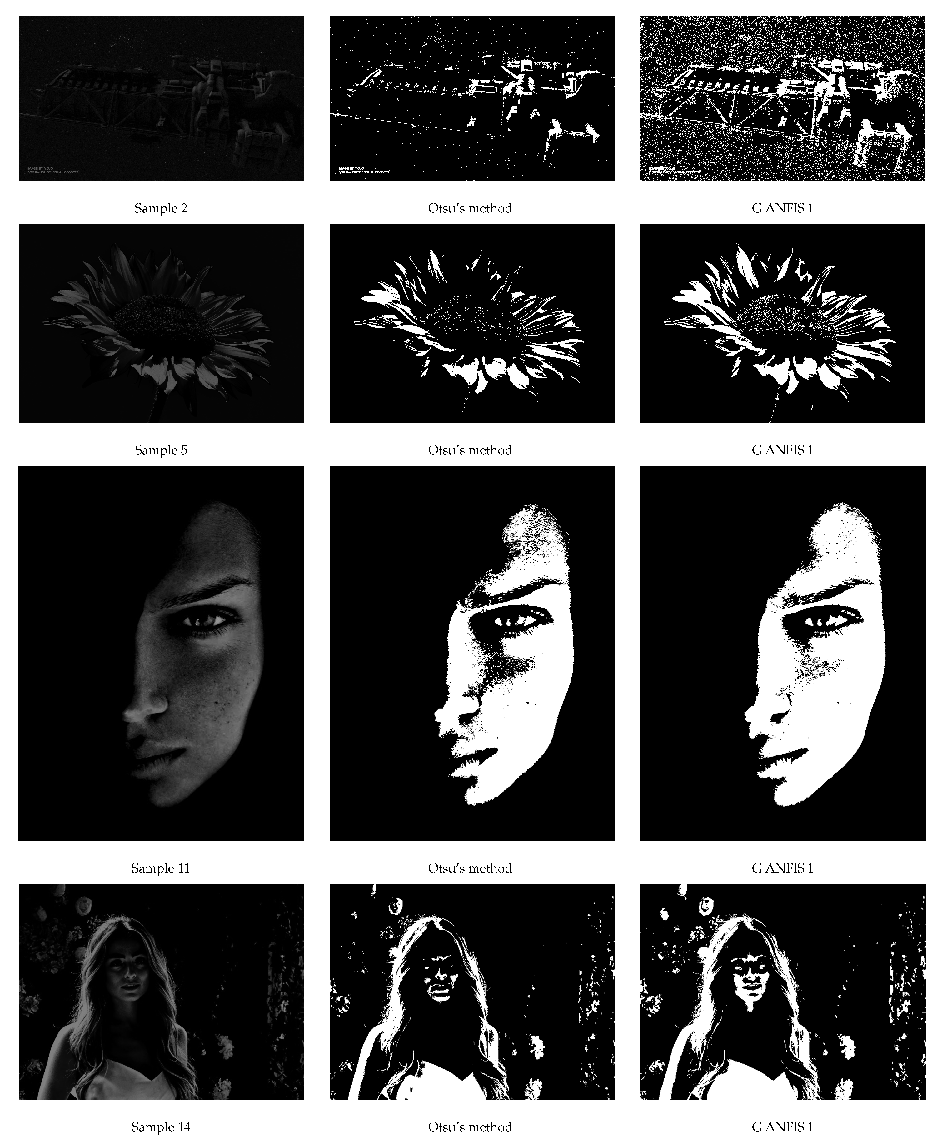
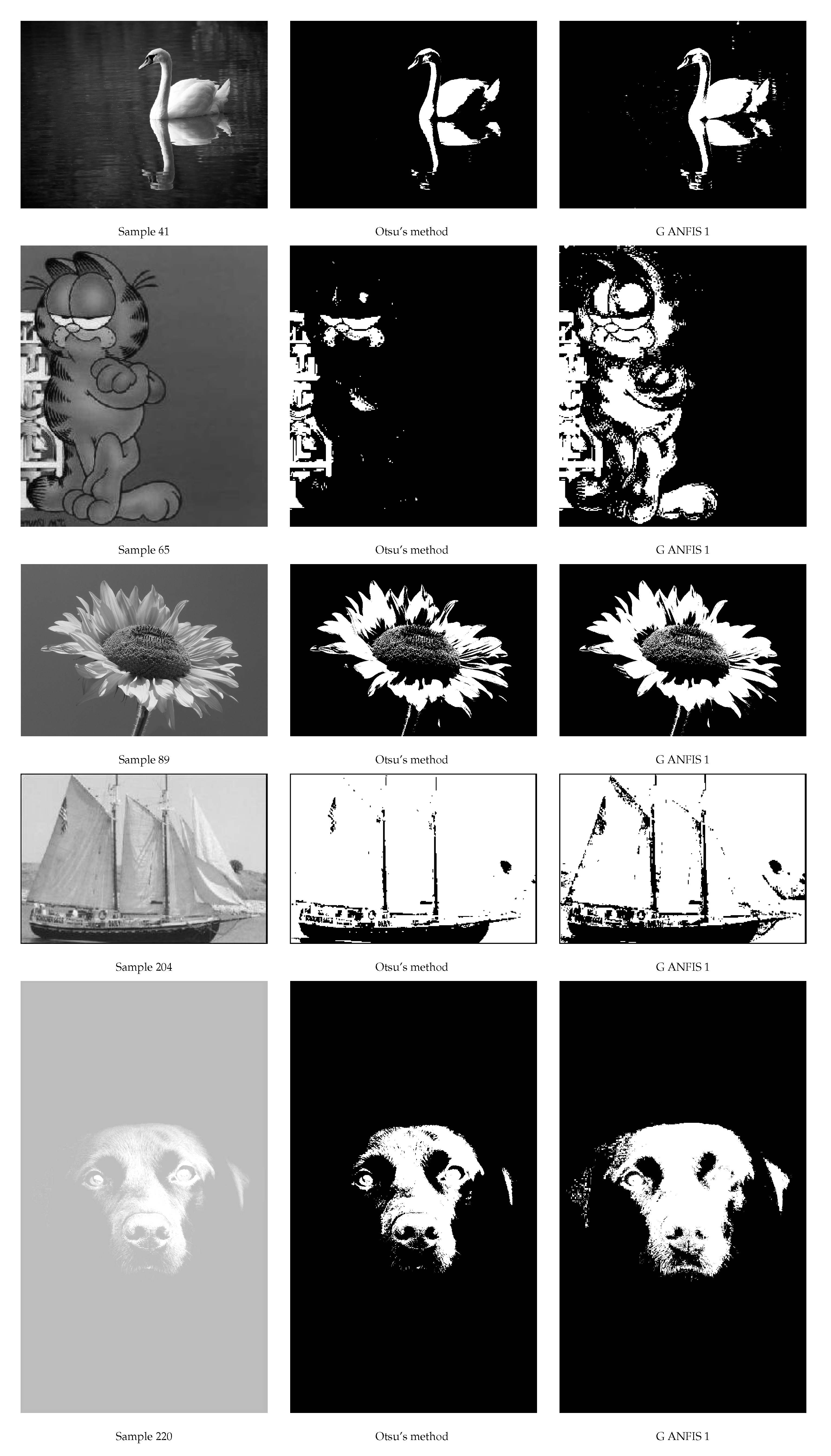
3. First Global Thresholding ANFIS

3.1. Data Construction and Initial Evaluation

In order to construct a proper database, we measured $s_1$, $s_2$, $s_3$, $s_4$, e (as described above) for a large set of images. We concluded with 252 images of various characteristics. These include famous paintings, random photos, noisy images, face images, comic pictures, object (one or many) images, landscapes and others. We didn’t focus on any specific domain since we mainly wanted to evaluate the proper transfer of information from our measures to a neural network. Our sources were the internet, articles of similar interest and the Caltech collections [108,109]. Some of these inputs constitute a brighter or a darker version of the same image since we wanted to create a set that covers all proper ranges (regarding the values of $s_1$ and $s_2$) based on our eight categories we saw in Section 2.3. We have to make clear that we don’t own most of these samples and that we used them because they were available for downloading and free of watermarks. Their copyright ownership is rather vague. Some of these have been used several times in similar research and others are uploaded in many sites without any further specific copyright details. Regardless, we downloaded and used these samples for research purposes only, so we hope that no one will object to this. However, if some owner of any particular image has any objections, we apologize in advance and we pledge to ask for his permission or to remove this specific sample.

In order to proceed to the training of our ANFIS, we needed of course a target t for each sample. Since there is not some publicly free, specialized database of the form “Image $im$-Proper threshold t”, we decided to initially set Otsu’s threshold as our t. This would help us to evaluate the potential of the whole process and to see if there is any meaning in continuing with it. Of course, based on our results in [2,20,21], we believed that most probably we would obtain some pretty good results. Thus, we trained an ANFIS with 252 vectors of the form $(s_1^v$, $s_2^v$, $s_3^v$,$s_4^v$, $e^v$, $t^v)$, $v=1\left(1\right)252$. These can can be seen using the following link: https://www.dropbox.com/s/tc297yl6crljgvc/GANFIS1Data.pdf?dl=0 and we will refer to them as data matrix 1. Samples are sorted according to $s_1$–$s_2$ and someone can see that almost half of our samples have $s_1<$$s_2$ and the others $s_1>$$s_2$. In other words, we made a substantial effort to have a good balance in our data. The smallest error occurred when we used triangular, bell-shaped and Gaussian membership functions and it was about $0.02$ (which is rather small, about five intensity values concerning grayscale images). We should also mention that we tried to use as input variables various combinations of $s_1$, $s_2$, $s_3$, $s_4$ and e (e.g., only $s_1$, $s_1$ and $s_2$, all of $s_i$, $s_1$, $s_2$ and e etc.). The best training was accomplished by using the maximum data, that is to say all of $s_1$, $s_2$, $s_3$, $s_4$ and e and it seems that each of them carries significant information concerning the attributes of the image. As fuzzy union and intersection, we used the default functions probor and product respectively since they returned the best results. From now on, all our results are obtained from systems trained with probor, product and triangular membership functions.

Thus, our first conclusion was that our ANFIS is trained very satisfactorily using these data. This derives not only from the small error but from the visual results as well. Of course, the latter cannot be displayed for obvious reasons. This was another proof that our measures are logical and applicable and that they can be related with thresholding very sufficiently. After this trial, we moved to the practical evaluation of the training of our ANFIS by separating a testing set of 50 images. These samples were picked randomly, but we made sure that all eight categories (from very dark to very bright) were properly represented. These images, like those of our training set, are of various sizes and characteristics and they are the samples listed in

Table 1. Testing samples.

Lines of data matrix 1 used as testing samples
2	5	7	11	14	18	20	21	25	33
34	35	36	41	43	50	63	65	87	89
101	111	115	123	124	128	132	137	142	152
155	177	178	184	190	193	201	204	209	210
213	220	222	229	231	238	239	240	247	251

. We trained our ANFIS using the remaining 202 samples. We used triangular membership functions and our error was again around $0.02$ (slightly smaller that before). Then, we used our trained ANFIS to binarize our testing set. Our results were from similar to indistinguishable compared to those of Otsu’s algorithm. Thus, based on these observations, we were convinced that fuzzy inclusion and entropy measures can effectively be used as inputs of the fuzzy inference system.

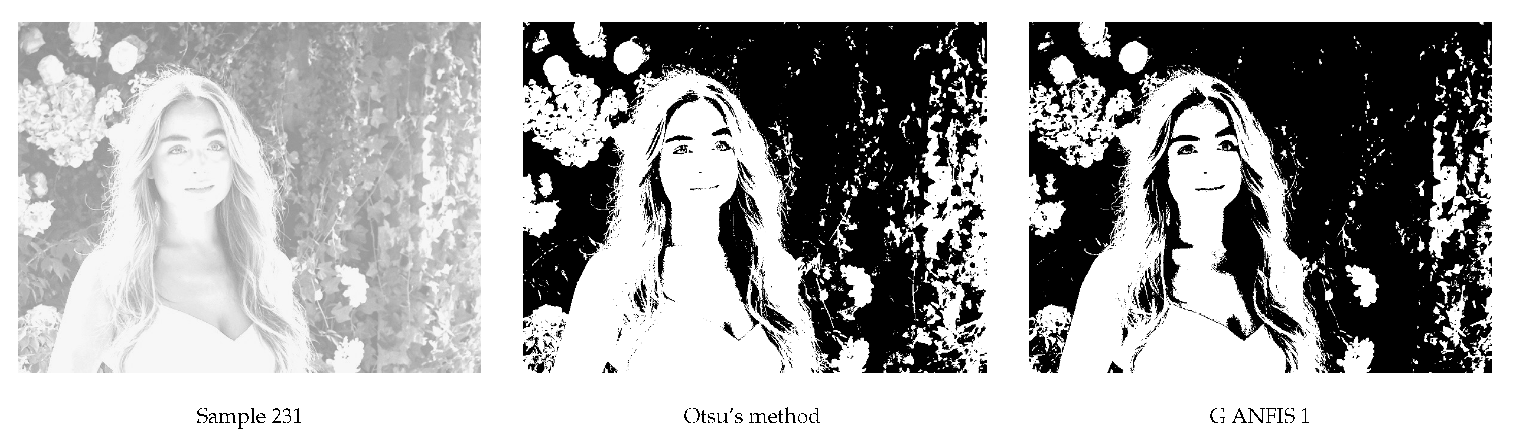
3.2. G(lobal) ANFIS 1—Adjusting Otsu’s Targets

Of course, our target was not just the reproduction of an existing global method via an ANFIS. The above procedure was made in order to examine the possibility of using our measures as inputs of the inference system. At the same time, it is important that we managed to approach a global method in this specific way because someone could interfere with the targets of the available data in order to “aid” this particular method in some “difficult” cases. Global algorithms which are free of sensitivity or bias parameters produce a specific result which cannot be further changed (unless, of course, someone proceeds to a modification or alteration of the whole methodology). Thus, we have to accept this result or turn to some more complex method (local or hybrid). On the other hand, if we use an inference system, we can experiment with the targets of our data set and modify specific results without having to mathematically redesign our whole algorithm. Certainly, the main difficulty of this process lies in the target setting, but this could derive from complicated analysis, someone’s experimentations or even simple observations. Let’s see an example of this.

During our data collection and the construction of our database, we observed some “imbalances” among Otsu’s thresholds, which could, to a certain degree, be responsible for our training error. What we mean is that some samples with relatively close values of $s_i$ and e had a rather large difference regarding their threshold obtained from Otsu’s method. For instance, let’s observe in Figure 1 the two images which correspond to lines 11 and 12 of our data matrix 1. In the matrix, we can see that their values—regarding $s_i$ and e—are very similar, whereas their threshold significantly differs ($0.13$ and $0.38$, respectively). Of course, Otsu’s method calculates the threshold of an image in a completely different course of thinking than ours. We need to clarify that we don’t want to argue on what is right or wrong or to question Otsu’s technique (one of the most respected methods there is) in any way. It is just what we mentioned: a different approach of the same problem.

Thus, in this sense, we felt that the threshold of sample 12 is rather high. If we set it closer to that of sample 11, let’s say cut half their difference, we can see what happens in Figure 2. We could say that, apart from the fact that the thresholds of the two samples come closer, the binarization of sample 12, using this lower value, is improved.

We made similar observations in other cases as well. For example, samples 39 and 41 (Figure 3) also have similar fuzzy inclusion and entropy values, but their thresholds are $0.26$ and $0.48$, respectively. We can see what happens if we lower the target of sample 41 (like described above) in Figure 4. By bringing the thresholding targets closer, we can see that we have obtained some further details of the swan.

Thus, based on these kinds of observations as well as on some visual experimentations, we readjusted the threshold-targets of our set and we trained our G(lobal) ANFIS 1. These new targets can be seen in the last column of our data matrix 1. Initially, we trained an ANFIS using all samples (1–252) to observe possible variation in our training error. Indeed, our error was reduced to almost half (around $0.01$). Then, we trained G ANFIS 1 using the same training set of 202 inputs and our new targets. Again, the error remained around $0.01$ and in Figure 5 we can see the differences in the binarizations of some samples of our testing set by G ANFIS 1 and Otsu’s algorithm. We should also mention that, due to samples of “extreme” illumination, sample 220 is a characteristic case, someone could add some “safety conditions”, e.g., we could set t always larger than $0.04$ or $0.05$ and lower than $0.95$ or $0.96$. This way, we can avoid the risk of an unacceptable binarization (like a completely black or white image) in case of such an “extreme” input.

As we can see, G ANFIS 1 helped us (slightly or significantly) with the thresholding of some dark images like samples 2, 5, 11, 14, some medium-lighted images like samples 41, 65, 89 and some bright images like samples 204, 220, 231. At the same time, we didn’t substantially harm all other results. The complete results of our testing set can be seen using the following link: https://www.dropbox.com/s/1qugs1l38hrg1up/GANFIS1Binarizations.pdf?dl=0. The binarizations of our training samples remained almost the same to those obtained before the target readjustment apart from a few samples (about 8 out of 202) where some more noticeable differences can be spotted. Regardless, we didn’t come with any totally unacceptable binarizations and we could say that G ANFIS 1 responded sufficiently (considering its purpose).

Though we didn’t alter a lot of our testing set binarizations, the above is just an indicative example of how someone could interfere with the database and alter specific results of a method without having to proceed to a modification of the algorithm itself. This was done based on simple observations and we are not some vision experts. We are sure that someone with more specialized knowledge could perform this much more efficiently and produce more distinguishable differences.

Next, we will see some part of our research on public databases which are related to image segmentation. This way, we will have the opportunity to set some more specialized targets and get some numerical results (besides the visual observation) as well.

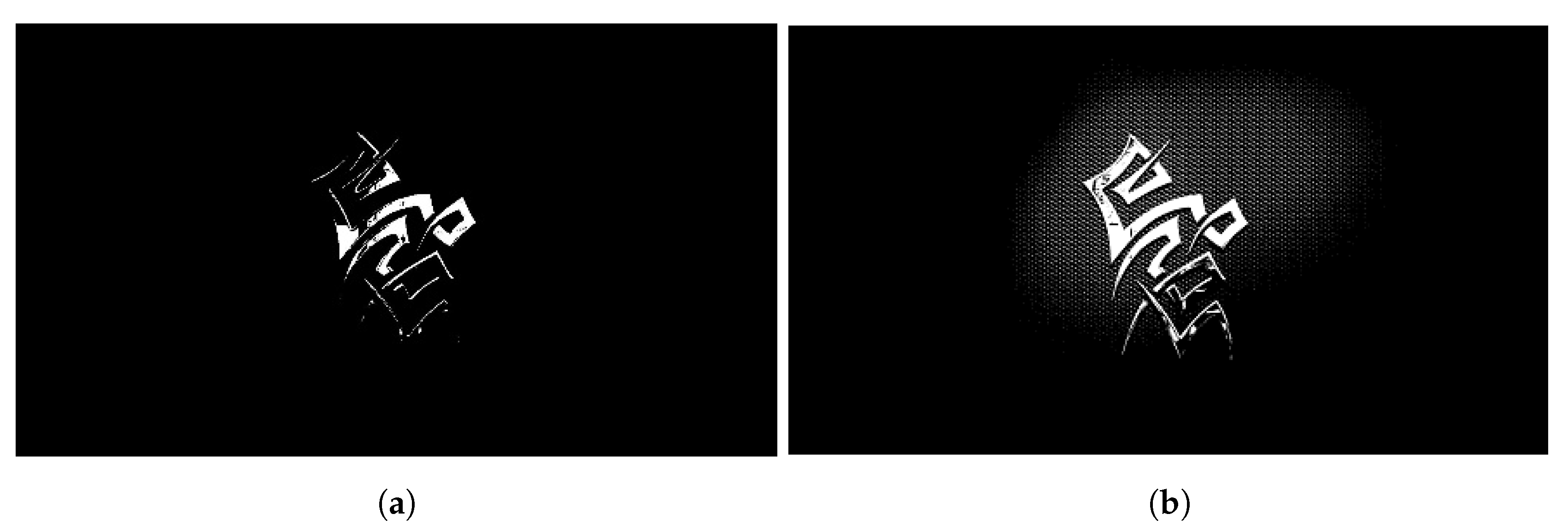
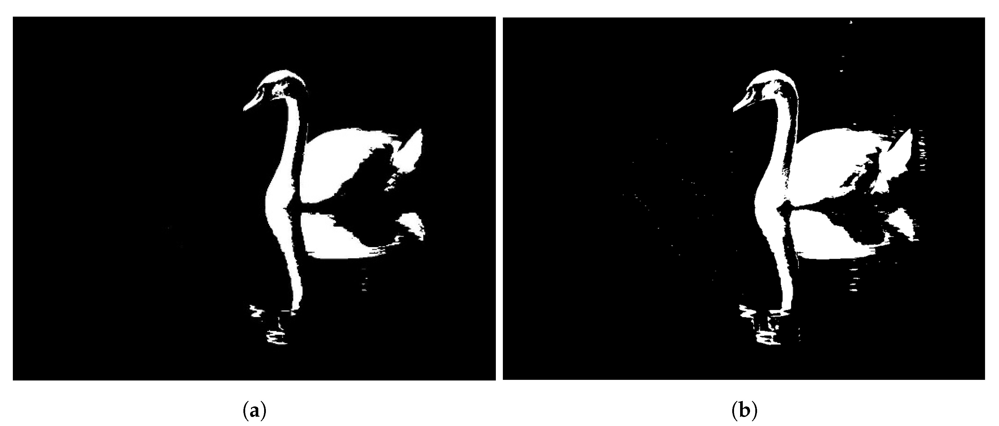
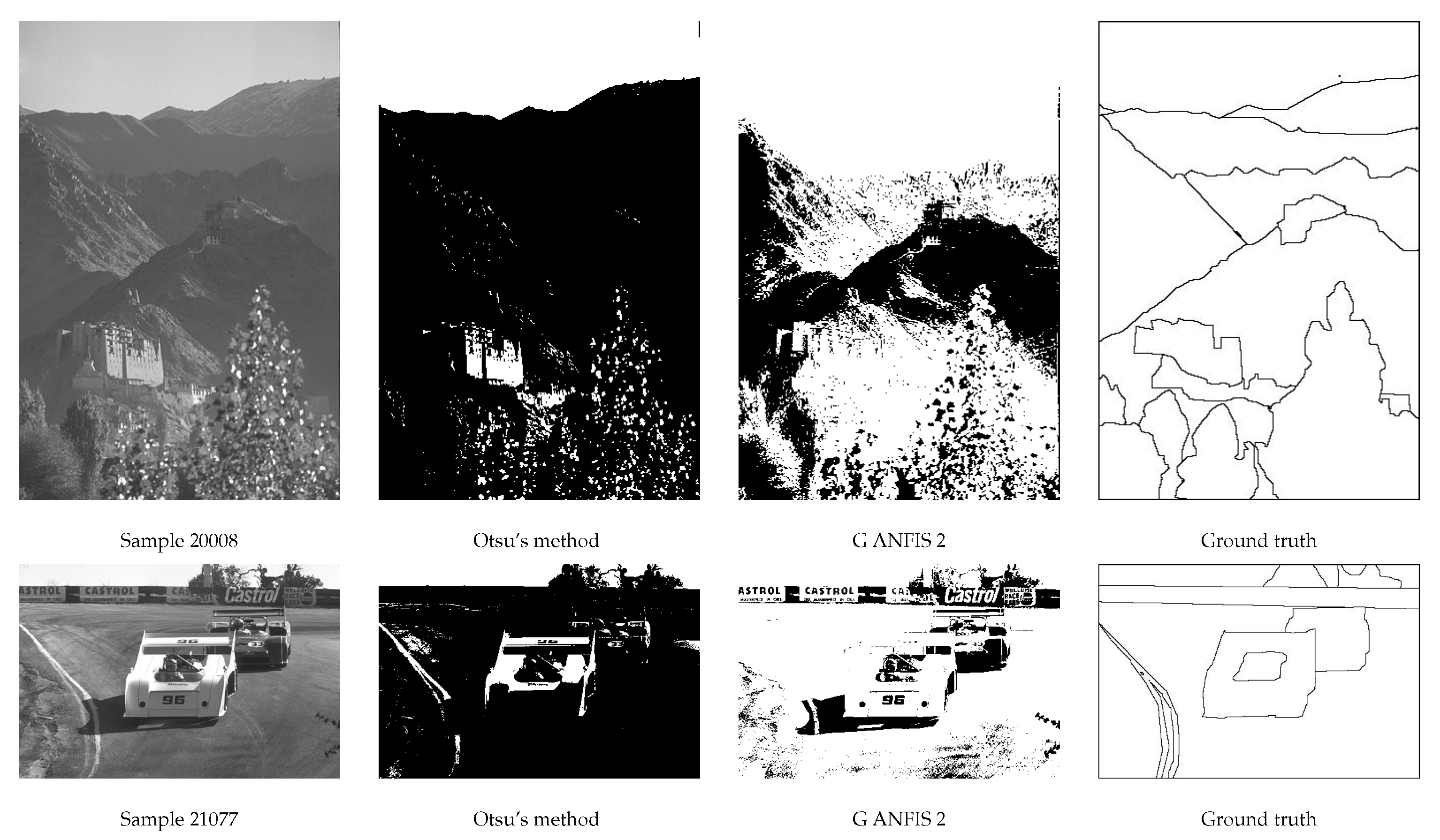
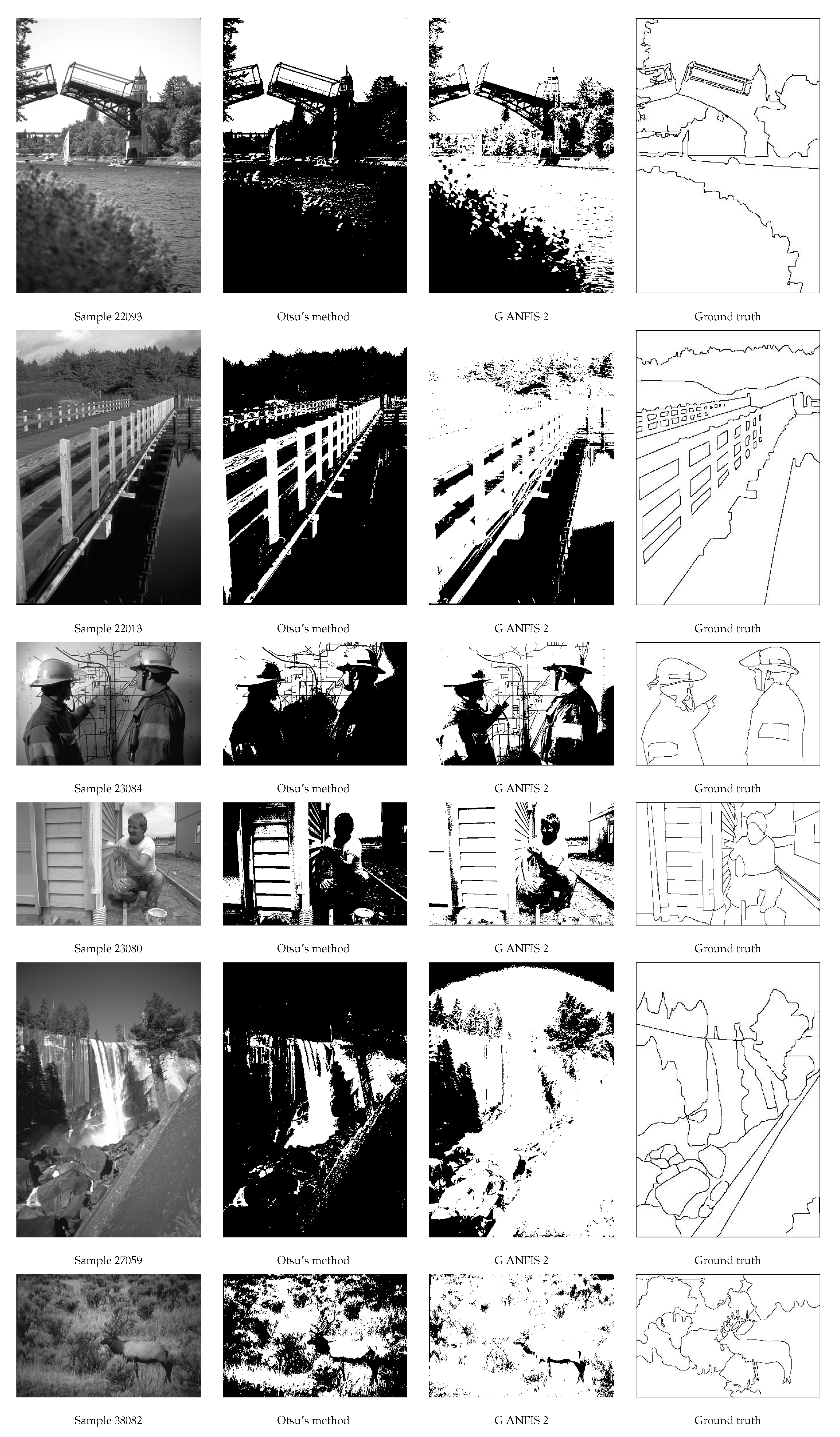
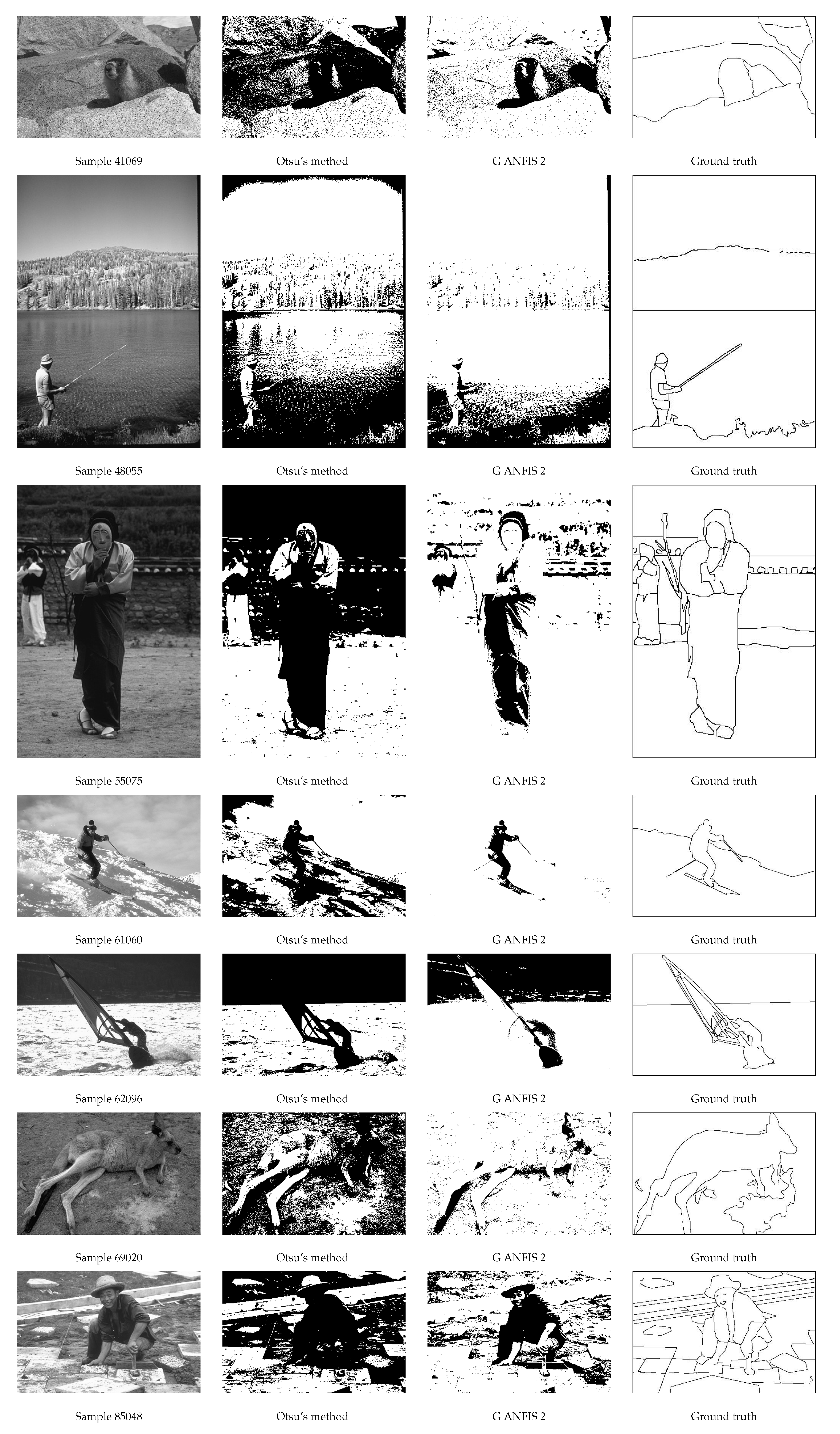
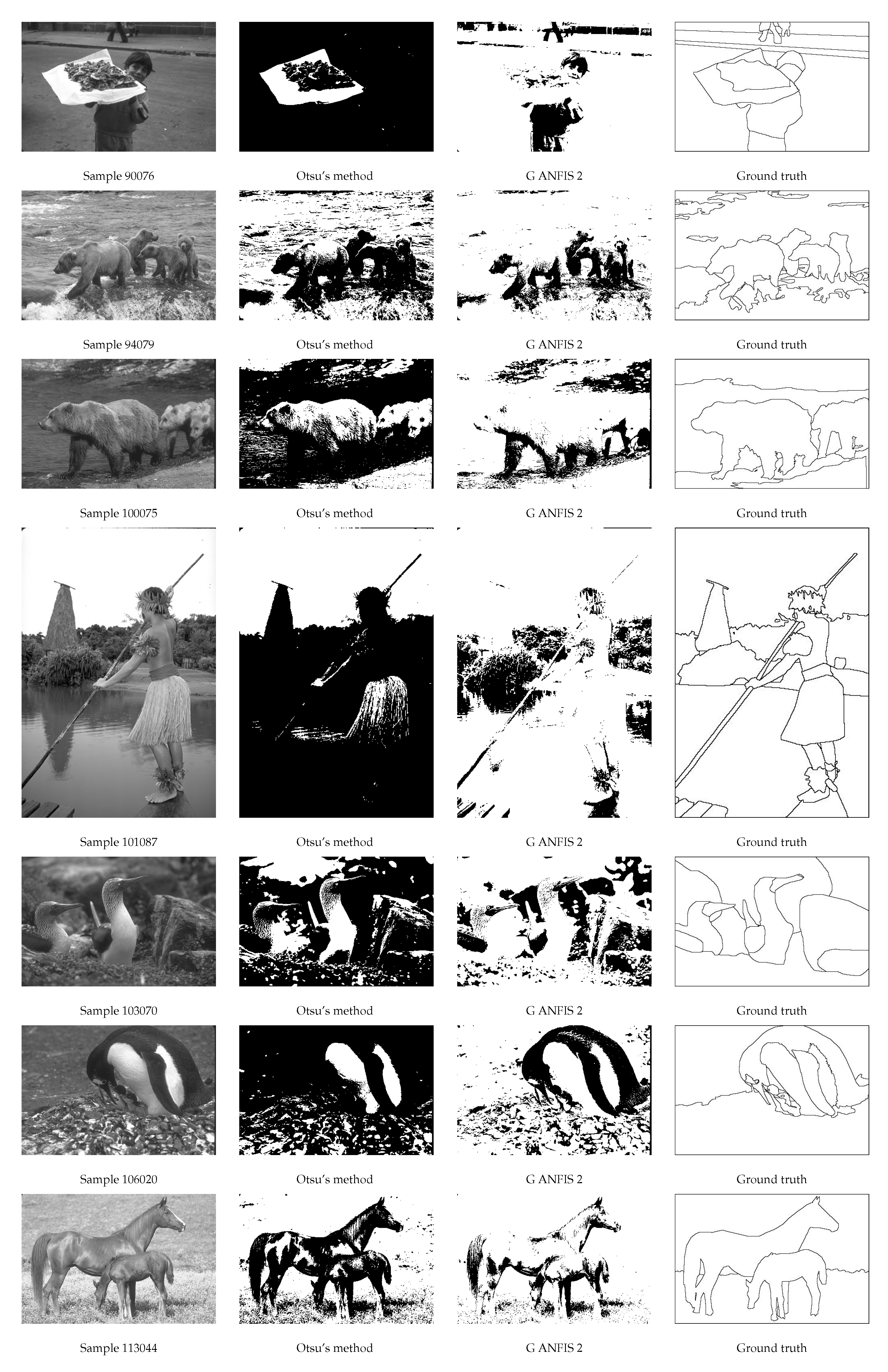
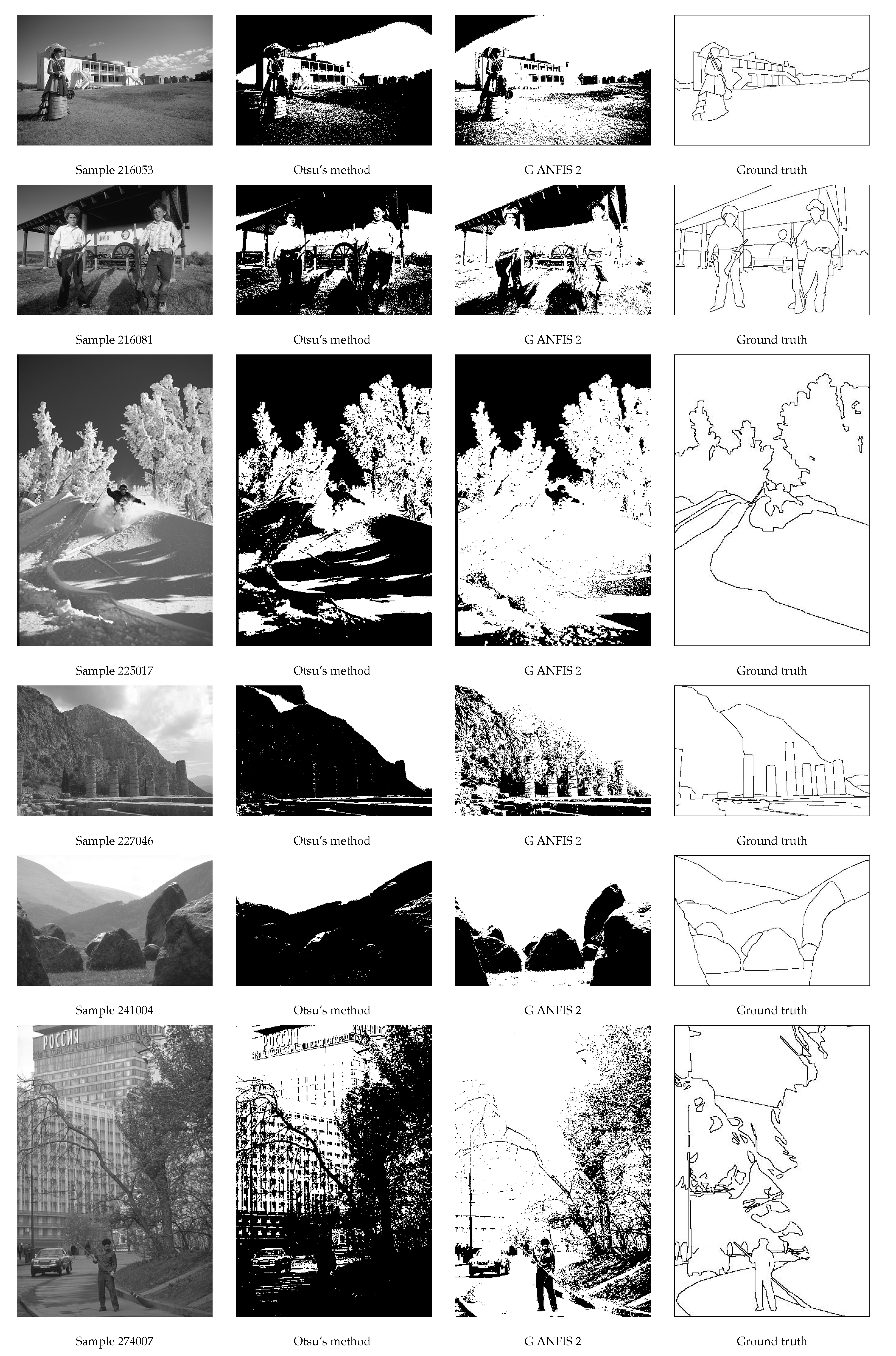
4. Second Global Thresholding ANFIS—Experimenting on Public Databases

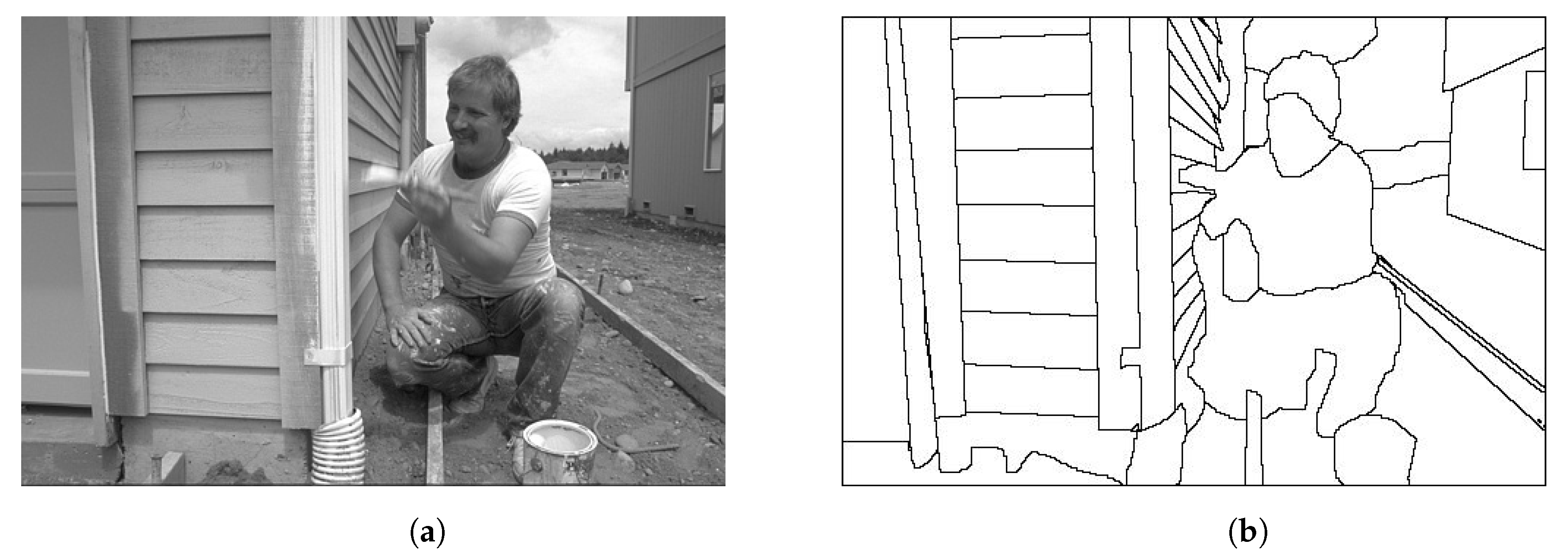
4.1. Public Databases Which We Used

Two distinguished online databases, which concern image segmentation and were suggested to us, are the “Berkeley Segmentation Data Set” [110] and the “Stanford Background Data Set” [111]. They are available for everyone and they offer a significant number of samples for algorithm testing. In fact, the Berkeley set 500 even has three separate sets of images (training, validation and testing) which seem very appropriate for our experimentations. However, the problem is that the ground truth of each sample is a set of several possible separations of the objects of the image according to human perception. This is far different from the single value ground truth we need and the Berkeley’s research team applies complex algorithms (including Contour plots and combinations of global and local thresholds) in order to identify the borders of the objects. In other words, the team is mainly focused on edge detection and the human annotations do not contain “filled” objects which occur when someone applies a single global threshold on the whole image. The database also provides some ground truth files in “Microsoft access table shortcut” form which we could not handle easily. Another problem with the samples of this database is the fact that almost all of them are “medium-lighted” (they belong in groups 3, 4, 7 and 8 according to the classification of Section 2.3 and just a few belong in group 2) and we cannot cover the whole required range (in terms of the difference $s_1$–$s_2$).

The Stanford database also shares the same features (their goal is very different than ours and the range is even narrower), but it accompanies each sample with some matrices in “txt” form (regarding the layers, regions and surfaces of the image) which can help in constructing a single value target. More specifically, the “regions” file contains a chromatic separation of the different objects of the image which helped us in producing some possible binarizations of the sample including “filled” (black) objects. Thus, we decided to train our ANFIS with data obtained from the Stanford database and test it on the samples (of similar lighting) of the Berkeley database. We believed that this could give our process some extra impartiality.

4.2. Data Set Construction of G(lobal) ANFIS 2

Let A be our image (from Stanford collection). Based on the “regions” matrix of A, we built two possible binarizations $S{B}_1$ and $S{B}_2$ of the image (black objects, no characteristics of the objects are visible) and we assigned to each sample two possible thresholds $t_1$ and $t_2$ based on the Jaccard similarity index between two $m\times n$ matrices $A=\left(a_{ij}\right)$ and $B=\left(b_{ij}\right)$. Its formula is:

$$J_g(A,B)=\frac{{\displaystyle \sum _{i,j}}min(a_{ij},b_{ij})}{{\displaystyle \sum _{i,j}}max(a_{ij},b_{ij})}.$$

(8)

Thresholds $t_1$ and $t_2$ where chosen in order to have the maximum value of $J_g(A,B_1)$ and $J_g(A,B_2)$ respectively. As our final target of image A, we set the average of these two thresholds. Thus, we resulted in 715 vectors of the form $(s_1^v$, $s_2^v$, $s_3^v$,$s_4^v$, $e^v$, $t^v)$, $v=1\left(1\right)715$. Since some targets seemed “awkward” and we believed that they were not appropriate for our inference system, we filtered these data (there were a lot of similar images in terms of fuzzy inclusion and entropy values) and we ended up with a total of 511 vectors. These can can be seen using the following link: https://www.dropbox.com/s/ld5xiz20tho4z7p/GANFIS2Data.pdf?dl=0. After this, we trained our G(lobal) ANFIS 2 with the filtered database and we proceeded to its testing on the Berkeley dataset.

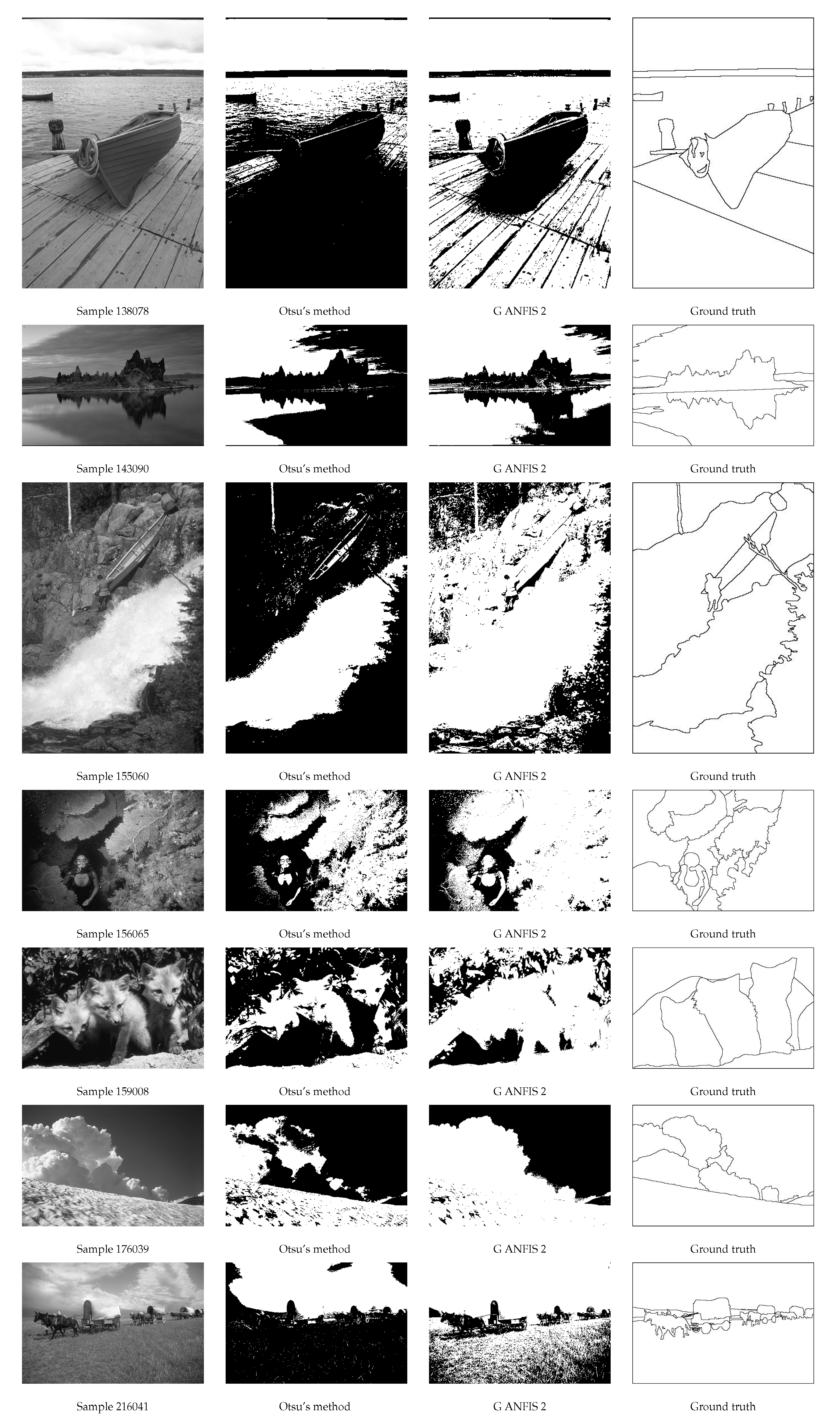
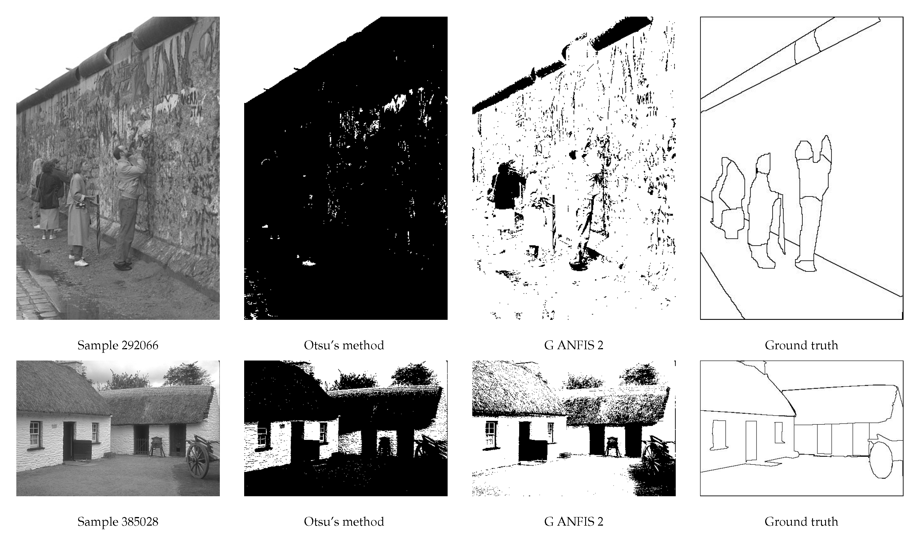
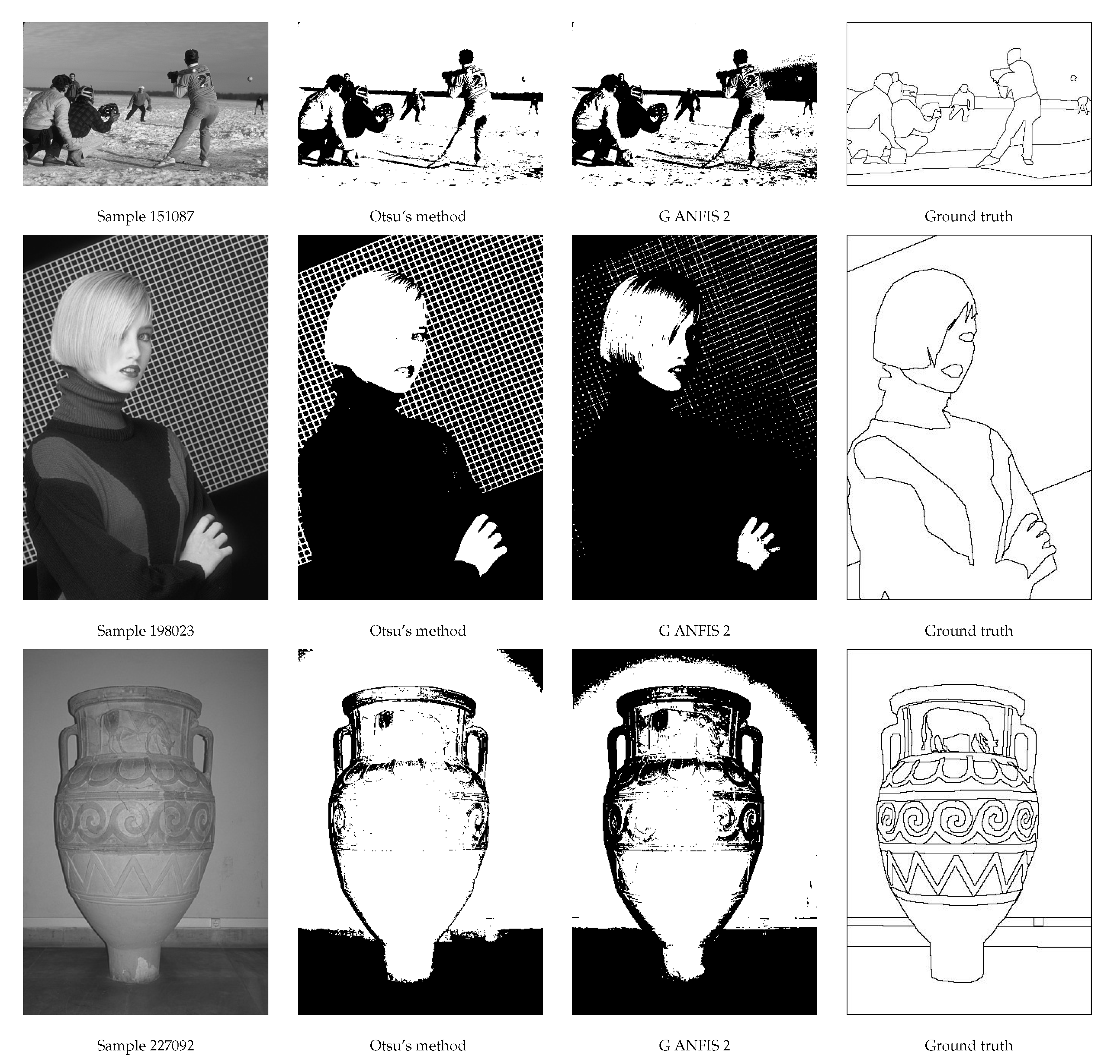
4.3. Testing of G ANFIS 2

For our testing, we used the BSD300 database (an older version of the latest BSD500 database) which contains 200 training images and 100 testing images. We used all 300 samples as our testing set which we will mention as BTS. We binarized these images with Otsu’s method and G ANFIS 2 and we evaluated the results based on the human segmentation of each image (we used the one with the most segments) which looks like the example in Figure 6.

Since, like we mentioned earlier, the range of our training set was not adequate, some samples of BTS were out of the range of G ANFIS 2. In addition, there were some images of BTS which were not represented in the training set (regarding the values of $s_i$ and e). Thus, we had to eliminate some images of BTS (the results were black or nearly black and white or nearly white binarizations) and conduct our measurements on the remaining images. We excluded 59 samples (out of the 300) and, for each of the remaining images, we measured the similarity of the binarized image with its corresponding human segmentation using two measures. The first was Jaccard’s index $J_g$ and the other was the structural similarity index (SSI) of MATLAB. Let’s call A our original sample, $GT$ its binary ground truth, $B_1$ its binarization with Otsu’s method and $B_2$ its binarization with G ANFIS 2. Out of the 241 samples, we had:

• 211 cases where $J_g(GT,B_2)>J_g(GT,B_1)$ (the difference $J_g(GT,B_2)-J_g(GT,B_1)$ varied from 0.76 to 0.01).
• 24 cases where $J_g(GT,B_2)<J_g(GT,B_1)$ (the difference $J_g(GT,B_1)-J_g(GT,B_2)$ varied from 0.17 to 0.01).
• 6 cases where the difference of $J_g(GT,B_1)$ and $J_g(GT,B_2)$ was zero.

All measurements were made on “tiff” formatted images and were rounded to two decimal numbers. Since we are talking of a lot of images, in

Table 2. Jaccard index measurements and their differences.

Sample	${\mathbf{J}}_{\mathbf{g}}(\mathbf{GT},{\mathbf{B}}_{\mathbf{2}})$	${\mathbf{J}}_{\mathbf{g}}(\mathbf{GT},{\mathbf{B}}_{\mathbf{1}})$	Difference	Sample	${\mathbf{J}}_{\mathbf{g}}(\mathbf{GT},{\mathbf{B}}_{\mathbf{2}})$	${\mathbf{J}}_{\mathbf{g}}(\mathbf{GT},{\mathbf{B}}_{\mathbf{1}})$	Difference
292066	0.87	0.11	0.76	90076	0.83	0.09	0.74
21077	0.81	0.14	0.67	135037	0.91	0.29	0.62
27059	0.72	0.13	0.59	108041	0.86	0.30	0.56
188063	0.90	0.39	0.51	106020	0.68	0.18	0.50
101087	0.82	0.33	0.49	109053	0.75	0.26	0.49
69020	0.88	0.39	0.48	46076	0.84	0.37	0.47
20008	0.67	0.21	0.46	385028	0.71	0.25	0.46
216066	0.81	0.36	0.45	100075	0.76	0.30	0.46
368078	0.68	0.25	0.43	103070	0.70	0.28	0.42
274007	0.74	0.33	0.41	55075	0.83	0.42	0.41
155060	0.72	0.31	0.41	216053	0.72	0.31	0.41
38082	0.86	0.47	0.39	187003	0.64	0.25	0.39
163085	0.77	0.38	0.39	23080	0.76	0.37	0.39
229036	0.68	0.30	0.38	138078	0.73	0.35	0.38
22013	0.62	0.25	0.37	183055	0.74	0.38	0.36
227046	0.70	0.33	0.37	216081	0.63	0.27	0.36
65132	0.72	0.36	0.36	41069	0.81	0.46	0.35
45077	0.72	0.36	0.36	105025	0.86	0.51	0.35
159008	0.72	0.37	0.35	178054	0.88	0.54	0.34
376043	0.60	0.26	0.34	69040	0.75	0.42	0.33
…	…	…	…	…	…	…	…
227092	0.54	0.69	−0.15	198023	0.12	0.29	−0.17

we present (in two columns) the forty first and the last two lines of the respective table. The full table (sorted by the difference $J_g(GT,B_2)-J_g(GT,B_1)$) can be seen using the following link: https://www.dropbox.com/s/4m52xo29dy00sva/JaccValuesandDifferences.pdf?dl=0.

As far as SSI is concerned, we had:

• 202 cases where $SSI(GT,B_2)>SSI(GT,B_1)$ (the difference $SSI(GT,B_2)-SSI(GT,B_1)$ varied from 0.53 to 0.01),
• 20 cases where $SSI(GT,B_2)<SSI(GT,B_1)$ (the difference $SSI(GT,B_1)-SSI(GT,B_2)$ varied from 0.11 to 0.01),
• 19 cases where the difference of $SSI(GT,B_1)$ and $SSI(GT,B_2)$ was zero.

Again, in

Table 3. Structural similarity index measurements and their differences.

Sample	$\mathbf{SSI}(\mathbf{GT},{\mathbf{B}}_{\mathbf{2}})$	$\mathbf{SSI}(\mathbf{GT},{\mathbf{B}}_{\mathbf{1}})$	Difference	Sample	$\mathbf{SSI}(\mathbf{GT},{\mathbf{B}}_{\mathbf{2}})$	$\mathbf{SSI}(\mathbf{GT},{\mathbf{B}}_{\mathbf{1}})$	Difference
108041	0.59	0.06	0.53	90076	0.58	0.06	0.52
135037	0.65	0.18	0.47	188063	0.61	0.16	0.45
61060	0.82	0.42	0.40	21077	0.43	0.06	0.37
27059	0.39	0.04	0.35	100075	0.44	0.09	0.35
69020	0.41	0.07	0.34	292066	0.40	0.07	0.33
101087	0.57	0.25	0.32	65132	0.42	0.10	0.32
38082	0.42	0.10	0.32	46076	0.56	0.25	0.31
105025	0.53	0.22	0.31	55075	0.53	0.24	0.29
94079	0.42	0.15	0.27	138032	0.33	0.06	0.27
156065	0.40	0.13	0.27	368078	0.35	0.08	0.27
163085	0.37	0.11	0.26	239096	0.42	0.15	0.27
106020	0.32	0.06	0.26	385028	0.33	0.08	0.25
159008	0.42	0.16	0.26	48055	0.57	0.32	0.25
109053	0.30	0.05	0.25	130026	0.31	0.06	0.25
41069	0.29	0.05	0.24	103070	0.35	0.10	0.25
176039	0.40	0.16	0.24	187003	0.30	0.07	0.23
225017	0.29	0.06	0.23	254054	0.30	0.07	0.23
143090	0.46	0.23	0.23	216053	0.38	0.16	0.22
62096	0.44	0.23	0.21	183055	0.40	0.18	0.22
178054	0.49	0.28	0.21	24063	0.55	0.35	0.20
…	…	…	…	…	…	…	…
227092	0.27	0.38	−0.11	151087	0.39	0.50	−0.11

, we present (in two columns) the forty first and the last two lines of the respective table. The full table (sorted by the difference $SSI(GT,B_2)-SSI(GT,B_1)$) can be seen using the following link: https://www.dropbox.com/s/okl9e126i9vyjxa/SSIValuesandDifferences.pdf?dl=0. Based on the values of Table 2 and Table 3, we can deduce that the binarizations of G ANFIS 2 were generally closer to our ground truth image compared to those of Otsu’s algorithm.

In other words, by setting our targets the way described above, we led our system to more bright and “empty” binarizations in order to approximate the human border sketching. Of course, like mentioned before, Berkeley’s research is completely different and far more complex than ours and it is impossible to replicate these results using a single threshold (a local approach, which is part of our current research, would be more appropriate). Nevertheless, it is again indicative of the benefit someone could have by setting the global targets on his own.

Besides the previous tables, we felt that it would be useful to present some visual results as well. Since we are talking of a lot of images, we chose some (from the union of the top 65 lines of our Table 2 or Table 3) which we believe that can depict this “approximation” more distinctly and we present them in Figure 7.

As far as our “bad” results are concerned, in Figure 8, we demonstrate the last lines (our “worst” binarizations according to the similarity indices) of Table 2 and Table 3. As someone can see, these do not significantly differ from the respective binarizations of Otsu’s algorithm.

5. Summary and Some Further Remarks

To sum up, in the previous two sections, we saw how fuzzy inclusion and entropy measures could efficiently be used as inputs of an inference system and how someone could benefit from setting the thresholding targets on his own. This can be hard regarding certain cases, but, on the other hand, it can help us produce specific results without having to alter an existing method or construct a new mathematical algorithm. Moreover, it could be implemented in various ways which vary from complicated analysis to simple observations. G ANFIS 1 and 2 were just some indicative evidence of how something like this could be done. Of course, in the case of G ANFIS 2, it would be impossible to reach the results of Berkeley’s and Stanford’s research teams using a single global threshold. Nevertheless, considering the circumstances, we think we managed to approach these results somehow better than Otsu’s algorithm or, at least, have more clear binarizations in many cases. The use of these data-sets was an interesting suggestion, however, their content is more related to our research on local and color segmentation. These and several other procedures consist parts of our current work and soon, we will be able to share some of its results.

Moreover, during this whole process which we described in the previous sections, we saw once again why is important to have a variety of fuzzy measures which could lead to new ideas and alternative ways of solving specific problems. We mention this because our algorithms in [2,20,21] couldn’t be implemented using any fuzzy inclusion function since most of them measure the inclusion of a fuzzy set A into ⌀ as zero. Under these circumstances, we wouldn’t be able to measure the “darkness” of an image and using only $s_1$ wouldn’t be enough for the proper connection between our measures and threshold t. The same applies here since without the values of $s_2$, our ANFIS returned inferior results to those we earlier saw. Another inclusion measure S that returns $S(A,⌀)\ne 0$ is Goguen’s index with the following formula:

$$S_g(A,B)=\frac{1}{\left|X\right|}\sum _{x\in X}min(1,1-m_A\left(x\right)+m_B\left(x\right)).$$

(9)

Its respective entropy measure is:

$$Eg\left(A\right)=\frac{2}{\left|X\right|}\sum _{x\in X}min(m_A\left(x\right),1-m_A\left(x\right)).$$

(10)

Of course, in this case, we have $S(A,⌀)=1-S(X,A)$. We experimented with measures (2), (3) and (9) and $S_1$ returned us the smaller error and the best results. This is the reason we used it in this presentation. Perhaps someone could achieve some better results using some other measure according to his own needs and targets.

Our theoretical work on the measures we introduced in [2] is constant and continuous; however, their application on real problems and their possible connection with other researches concerning such fuzzy functions could offer us a lot of valuable information regarding their potential as well as their behavior. Some procedures which often deal with fuzzy inclusion or entropy measurements concern feature selection, fuzzy classification, fuzzy controllers, fuzzy rules and similarity measures. There are several presentations of this kind (e.g., [112,113,114,115,116,117,118,119] are a few recent) and it would be extremely useful if a certain part of our work could be connected with (or even included in) some of these studies. This would be a significant aid to our research and we could better comprehend the attributes and the performance of these measures.

6. Conclusions

In this paper, we continued our work in [2,20,21] and we presented an alternative approach to the thresholding problem using the ANFIS method to automatically connect our fuzzy inclusion and entropy measures with the wanted threshold of the image. Like in all of our previous presentations, we avoided any kind of analysis of our input (depending on its histogram) and bias or sensitivity parameters. All we need is a simple transformation of the image into a fuzzy set along with some simple measurements and, once again, we can see why it is important to have a variety of fuzzy measures since this could lead us to new ways of dealing with specific problems.

Of course, our research is continued and, as we mentioned, we have already used this ANFIS approach on a local level as well. Certainly, in this case, the process of data collection is different, but again, our method has returned some very adequate results (at least for the kind of images we used in [20,21] which are mainly degraded or unevenly illuminated documents). These are definitely going to be displayed in a future presentation along with some other results which derived from our current experimentations on several domains of images. At the same time, we also continue our theoretical research on our measures and we already have several ideas of combining them with other relative works which deal with fuzzy inclusion and entropy or include processes which are connected with these concepts.

References

1. Sezgin, M.; Sankur, B. Survey over image thresholding techniques and quantitative performance evaluation. J. Electron. Imaging 2004, 13, 146–168. [Google Scholar] [CrossRef]
2. Bogiatzis, A.; Papadopoulos, B. Producing Fuzzy Inclusion and Entropy Measures and Their Application on Global Image Thresholding. B.K. Evol. Syst. 2018, 9, 331–353. [Google Scholar] [CrossRef]
3. Young, V.R. Fuzzy subsethood. Fuzzy Sets Syst. 1996, 77, 371–384. [Google Scholar] [CrossRef]
4. Kosko, B. Fuzzy Thinking: The New Science of Fuzzy Logic; Hyperion: New York, NY, USA, 1993; ISBN 0-7868-8021-X. [Google Scholar]
5. Kosko, B.; Isaka, S. Fuzzy Logic. Sci. Am. 1993, 269, 76–81. [Google Scholar] [CrossRef]
6. Kosko, B. Neural Networks and Fuzzy Systems: A Dynamical Systems Approach to Machine Intelligence; Prentice-Hall: Englewood Cliffs, NJ, USA, 1992; ISBN 9780136114352. [Google Scholar]
7. Boulmakoul, A.; Laarabi, M.H.; Sacile, R.; Garbolino, E. An original approach to ranking fuzzy numbers by inclusion index and Bitset Encoding. Fuzzy Optim. Decis. Mak. 2017, 16, 23–49. [Google Scholar] [CrossRef]
8. Bronevich, A.G.; Rozenberg, I.N. Ranking probability measures by inclusion indices in the case of unknown utility function. Fuzzy Optim. Decis. Mak. 2014, 13, 49–71. [Google Scholar] [CrossRef]
9. Burillo, P.; Frago, N.; Fuentes, R. Inclusion grade and fuzzy implication operators. Fuzzy Set. Syst. 2000, 114, 417–429. [Google Scholar] [CrossRef]
10. Cheng, W.C. Conditional Fuzzy Entropy of Maps in Fuzzy Systems. Theory Comput. Syst. 2011, 48, 767–780. [Google Scholar] [CrossRef]
11. Cornelis, C.; Van der Donck, C.; Kerre, E. Sinha–Dougherty approach to the fuzzification of set inclusion revisited. Fuzzy Set. Syst. 2003, 134, 283–295. [Google Scholar] [CrossRef]
12. Dey, V.; Pratihar, D.K.; Datta, G.L. Genetic algorithm-tuned entropy-based fuzzy C-means algorithm for obtaining distinct and compact clusters. Fuzzy Optim. Decis. Mak. 2011, 10, 153–166. [Google Scholar] [CrossRef]
13. Jung, D.; Choi, J.W.; Park, W.J.; Lee, S. Quantitative comparison of similarity measure and entropy for fuzzy sets. J. Cent. South Univ. Technol. 2011, 18, 2045–2049. [Google Scholar] [CrossRef]
14. Lukka, P. Feature selection using fuzzy entropy measures with similarity classifier. Expert Syst. Appl. 2011, 38, 4600–4607. [Google Scholar] [CrossRef]
15. Palanisamy, C.; Selvan, S. Efficient subspace clustering for higher dimensional data using fuzzy entropy. J. Syst. Sci. Syst. Eng. 2009, 18, 95–110. [Google Scholar] [CrossRef]
16. Scozzafava, R.; Vantaggi, B. Fuzzy inclusion and similarity through coherent conditional probability. Fuzzy Sets Syst. 2009, 160, 292–305. [Google Scholar] [CrossRef]
17. Sussner, P.; Valle, M.E. Classification of Fuzzy Mathematical Morphologies Based on Concepts of Inclusion Measure and Duality. J. Math. Imaging Vis. 2008, 32, 139–159. [Google Scholar] [CrossRef]
18. Zhang, H.; Yang, S. Inclusion measure for typical hesitant fuzzy sets, the relative similarity measure and fuzzy entropy. Soft Comput. 2016, 20, 1277–1287. [Google Scholar] [CrossRef]
19. Zhou, R.; Yang, Z.; Yu, M.; Ralescu, D.A. A portfolio optimization model based on information entropy and fuzzy time series. Fuzzy Optim. Decis. Mak. 2015, 1, 381–397. [Google Scholar] [CrossRef]
20. Bogiatzis, A.; Papadopoulos, B. Local Thresholding of Degraded or Unevenly Illuminated Documents Using Fuzzy Inclusion and Entropy Measures. B.K. Evol. Syst. 2019. [Google Scholar] [CrossRef]
21. Bogiatzis, A.; Papadopoulos, B. Binarization of Texts with Varying Lighting Conditions Using Fuzzy Inclusion and Entropy Measures. AIP Conf. Proc. 2018, 1978. [Google Scholar] [CrossRef]
22. Halada, L.; Osokov, G.A. Histogram concavity analysis by quasicurvature. Comput. Artif. Intell. 1987, 6, 523–533. [Google Scholar]
23. Rosenfeld, A.; De la Torre, P. Histogram concavity analysis as an aid in threshold selection. IEEE Trans. Syst. Man Cybern. 1983, 13. [Google Scholar] [CrossRef]
24. Sahasrabudhe, S.C.; Gupta, K.S.D. A valley-seeking threshold selection technique. Comput. Vis. Image Underst. 1992, 56, 55–65. [Google Scholar]
25. Weszka, J.; Rosenfeld, A. Histogram modification for threshold selection. IEEE Trans. Syst. Man Cybern. 1979, 9, 38–52. [Google Scholar] [CrossRef]
26. Weszka, J.; Rosenfeld, A. Threshold evaluation techniques. IEEE Trans. Syst. Man Cybern. 1978, 8, 622–629. [Google Scholar] [CrossRef]
27. Carlotto, M.J. Histogram analysis using a scale-space approach. IEEE Trans. Pattern Anal. Mach. Intell. 1987, 9, 121–129. [Google Scholar] [CrossRef] [PubMed]
28. Olivo, J.C. Automatic threshold selection using the wavelet transform. Graph. Models Image Process. 1994, 56, 205–218. [Google Scholar] [CrossRef]
29. Sezan, M.I. A peak detection algorithm and its application to histogram-based image data reduction. Comput. Vis. Graph. Image Process. 1990, 49, 36–51. [Google Scholar] [CrossRef]
30. Cai, J.; Liu, Z.Q. A new thresholding algorithm based on all-pole model. In Proceedings of the Fourteenth International Conference on Pattern Recognition, Brisbane, Queensland, Australia, 20 August 1998; Volume 1, pp. 34–36. [Google Scholar] [CrossRef]
31. Guo, R.; Pandit, S.M. Automatic threshold selection based on histogram modes and a discriminant criterion. Mach. Vis. Appl. 1998, 10, 331–338. [Google Scholar] [CrossRef]
32. Kampke, T.; Kober, R. Nonparametric optimal binarization. In Proceedings of the Fourteenth International Conference on Pattern Recognition, Brisbane, Queensland, Australia, 20 August 1998; Volume 1, pp. 27–29. [Google Scholar] [CrossRef]
33. Ramesh, N.; Yoo, J.H.; Sethi, I.K. Thresholding based on histogram approximation. Proc. Vis. Image Signal Process. 1995, 142, 271–279. [Google Scholar] [CrossRef]
34. Leung, C.K.; Lam, F.K. Performance analysis of a class of iterative image thresholding algorithms. Pattern Recogn. 1996, 29, 1523–1530. [Google Scholar] [CrossRef]
35. Ridler, T.W.; Calvard, C. Picture thresholding using an iterative selection method. IEEE Trans. Syst. Man Cybern. 1978, 8, 630–632. [Google Scholar] [CrossRef]
36. Trussel, H.J. Comments on picture thresholding using iterative selection method. IEEE Trans. Syst. Man Cybern. 1979, 9, 311. [Google Scholar] [CrossRef]
37. Yanni, M.K.; Horne, E. A new approach to dynamic thresholding. In Proceedings of the EUSIPCO’94: 9th European European Signal Processing Conference, Edinburgh, UK, 13–16 September 1994; Volume 1, pp. 34–41. [Google Scholar]
38. Cho, S.; Haralick, R.; Yi, S. Improvement of Kittler and Illingworths’s minimum error thresholding. Pattern Recogn. 1989, 22, 609–617. [Google Scholar] [CrossRef]
39. Kittler, J.; Illingworth, J. Minimum error thresholding. Pattern Recogn. 1986, 19, 41–47. [Google Scholar] [CrossRef]
40. Jawahar, C.V.; Biswas, P.K.; Ray, A.K. Investigations on fuzzy thresholding based on fuzzy clustering. Pattern Recogn. 1997, 30, 1605–1613. [Google Scholar] [CrossRef]
41. Otsu, N. A threshold selection method from gray level histograms. IEEE Trans. Syst. Man Cybern. 1979, 9, 62–66. [Google Scholar] [CrossRef]
42. Pal, S.K.; King, R.A.; Hashim, A.A. Automatic gray level thresholding through index of fuzziness and entropy. Pattern Recogn. Lett. 1983, 1, 141–146. [Google Scholar] [CrossRef]
43. Johannsen, G.; Bille, J. A threshold selection method using information measures. In Proceedings of the ICPR’82: 6th International Conference on Pattern Recognition, Munich, Germany, 19–22 October 1982; pp. 140–143. [Google Scholar]
44. Kapur, J.N.; Sahoo, P.K.; Wong, A.K.C. A new method for gray-level picture thresholding using the entropy of the histogram. Graph. Models Image Process. 1985, 29, 273–285. [Google Scholar] [CrossRef]
45. Pun, T. Entropic thresholding: A new approach. Comput. Graph. Image Process. 1981, 16, 210–239. [Google Scholar] [CrossRef]
46. Sahoo, P.; Wilkins, C.; Yeager, J. Threshold selection using Renyi’s entropy. Pattern Recogn. 1997, 30, 71–84. [Google Scholar] [CrossRef]
47. Yen, J.C.; Chang, F.J.; Chang, S. A new criterion for automatic multilevel thresholding. IEEE Trans. Image Process. 1995, 4, 370–378. [Google Scholar] [CrossRef] [PubMed]
48. Brink, A.D.; Pendock, N.E. Minimum cross entropy threshold selection. Pattern Recogn. 1996, 29, 179–188. [Google Scholar] [CrossRef]
49. Li, C.H.; Tam, P.K.S. An iterative algorithm for minimumcross-entropy thresholding. Pattern Recogn. Lett. 1998, 19, 771–776. [Google Scholar] [CrossRef]
50. Li, C.H.; Lee, C.K. Minimum cross-entropy thresholding. Pattern Recogn. 1993, 26, 617–625. [Google Scholar] [CrossRef]
51. Pal, N.R. On minimum cross-entropy thresholding. Pattern Recogn. 1996, 29, 575–580. [Google Scholar] [CrossRef]
52. Hertz, L.; Schafer, R.W. Multilevel thresholding using edge matching. Comput. Vis. Graph. Image Process. 1988, 44, 279–295. [Google Scholar] [CrossRef]
53. Cheng, S.C.; Tsai, W.H. A neural network approach of the moment-preserving technique and its application to thresholding. IEEE Trans. Comput. 1993, 42, 501–507. [Google Scholar] [CrossRef]
54. Delp, E.J.; Mitchell, O.R. Moment-preserving quantization. IEEE Trans. Commun. 1991, 39, 1549–1558. [Google Scholar] [CrossRef]
55. Tsai, W.H. Moment-preserving thresholding: A new approach. Graph. Models Image Process. 1985, 29, 377–393. [Google Scholar] [CrossRef]
56. Pal, S.K.; Rosenfeld, A. Image enhancement and thresholding by optimization of fuzzy compactness. Pattern Recogn. Lett. 1988, 7, 77–86. [Google Scholar] [CrossRef]
57. Rosenfeld, A. The fuzzy geometry of image subsets. Pattern Recogn. Lett. 1984, 2, 311–317. [Google Scholar] [CrossRef]
58. O’Gorman, L. Binarization and multithresholding of document images using connectivity. Graph. Models Image Process. 1994, 56, 494–506. [Google Scholar] [CrossRef]
59. Liu, Y.; Srihari, S.N. Document image binarization based on texture analysis. Proc. SPIE 1994, 2181, 254–263. [Google Scholar] [CrossRef]
60. Pikaz, A.; Averbuch, A. Digital image thresholding based on topological stable state. Pattern Recogn. 1996, 29, 829–843. [Google Scholar] [CrossRef]
61. Murthy, C.A.; Pal, S.K. Fuzzy thresholding: A mathematical framework, bound functions and weighted moving average technique. Pattern Recogn. Lett. 1990, 11, 197–206. [Google Scholar] [CrossRef]
62. Ramar, K.; Arunigam, S.; Sivanandam, S.N.; Ganesand, L.; Manimegalai, D. Quantitative fuzzy measures for threshold selection. Pattern Recogn. Lett. 2000, 21, 1–7. [Google Scholar] [CrossRef]
63. Kirby, R.L.; Rosenfeld, A. A Note on the Use of (Gray Level, Local Average Gray Level) Space as an Aid in Threshold Selection. IEEE Trans. Syst. Man Cybern. 1979, 9, 860–864. [Google Scholar]
64. Fekete, G.; Eklundh, J.O.; Rosenfeld, A. Relaxation: Evaluation and applications. IEEE Trans. Pattern Anal. Mach. Intell. 1981, 3, 459–469. [Google Scholar] [CrossRef] [PubMed]
65. Rosenfeld, A.; Smith, R. Thresholding using relaxation. IEEE Trans. Pattern Anal. Mach. Intell. 1981, 3, 598–606. [Google Scholar] [CrossRef] [PubMed]
66. Wu, A.Y.; Hong, T.H.; Rosenfeld, A. Threshold selection using quadtrees. IEEE Trans. Pattern Anal. Mach. Intell. 1982, 4, 90–94. [Google Scholar] [CrossRef] [PubMed]
67. Ahuja, N.; Rosenfeld, A. A note on the use of second-order gray level statistics for threshold selection. IEEE Trans. Syst. Man Cybern. 1978, 8, 895–898. [Google Scholar] [CrossRef]
68. Chanda, B.; Majumder, D.D. A note on the use of gray level co-occurrence matrix in threshold selection. Signal Process. 1988, 15, 149–167. [Google Scholar] [CrossRef]
69. Chang, C.; Chen, K.; Wang, J.; Althouse, M.L.G. A relative entropy based approach in image thresholding. Pattern Recogn. 1994, 27, 1275–1289. [Google Scholar] [CrossRef]
70. Lie, W.N. An efficient threshold-evaluation algorithm for image segmentation based on spatial gray level cooccurrences. Signal Process. 1993, 33, 121–126. [Google Scholar] [CrossRef]
71. Abutaleb, A.S. Automatic thresholding of gray-level pictures using two-dimensional entropy. Comput. Vis. Graph. Image Process. 1989, 47, 22–32. [Google Scholar] [CrossRef]
72. Brink, A.D. Minimum spatial entropy threshold selection. IEE Proc. Vis.Image Signal Process. 1995, 142, 128–132. [Google Scholar] [CrossRef]
73. Brink, A.D. Thresholding of digital images using two-dimensional entropies. Pattern Recogn. 1992, 25, 803–808. [Google Scholar] [CrossRef]
74. Cheng, H.D.; Chen, Y.H. Thresholding based on fuzzy partition of 2D histogram. In Proceedings of the Fourteenth International Conference on Pattern Recognition, Brisbane, Queensland, Australia, 20 August 1998; pp. 1616–1618. [Google Scholar] [CrossRef]
75. Li, L.; Gong, J.; Chen, W. Gray-level image thresholding based on fisher linear projection of two-dimensional histogram. Pattern Recogn. 1997, 30, 743–749. [Google Scholar] [CrossRef]
76. Pal, N.R.; Pal, S.K. Entropic thresholding. Signal Process. 1989, 16, 97–108. [Google Scholar] [CrossRef]
77. Brink, A.D. Gray level thresholding of images using a correlation criterion. Pattern Recogn. Lett. 1989, 9, 335–341. [Google Scholar] [CrossRef]
78. Cheng, H.D.; Chen, Y.H. Fuzzy partition of two-dimensional histogram and its application to thresholding. Pattern Recogn. 1999, 32, 825–843. [Google Scholar] [CrossRef]
79. Leung, C.K.; Lam, F.K. Maximum a posteriori spatial probability segmentation. IEE Proc. Vis. Image Signal Process. 1997, 144, 161–167. [Google Scholar] [CrossRef]
80. Friel, N.; Molchanov, I.S. A new thresholding technique based on random sets. Pattern Recogn. 1999, 32, 1507–1517. [Google Scholar] [CrossRef]
81. Bernsen, J. Dynamic thresholding of gray level images. In Proceedings of the International Conference on Pattern Recognition (ICPR’86), Berlin, Germany, 27–31 October 1986; pp. 1251–1255. [Google Scholar]
82. Niblack, W. An Introduction to Image Processing; Prentice-Hall: Englewood Cliffs, NJ, USA, 1986; ISBN 0134806743. [Google Scholar]
83. Sauvola, J.; Pietaksinen, M. Adaptive document image binarization. Pattern Recogn. 2000, 33, 225–236. [Google Scholar] [CrossRef]
84. Yanowitz, S.D.; Bruckstein, A.M. A new method for image segmentation. Comput. Graph. Image Process. 1989, 46, 82–95. [Google Scholar] [CrossRef]
85. Othman, A.A.; Tizhoosh, H.R. Image thresholding using neural network. In Proceedings of the 10th International Conference on Intelligent Systems Design and Applications, Cairo, Egypt, 29 November–1 December 2010; pp. 1159–1164. [Google Scholar] [CrossRef]
86. Ahmed, M.N.; Farag, A.A. Two-stage neural network for volume segmentation of medical images. Pattern Recogn. Lett. 1997, 18, 1143–1151. [Google Scholar] [CrossRef]
87. Chang, C.Y.; Chung, P.C. Medical image segmentation using a contextual-constraint-based Hopfield neural cube. Image Vis. Comput. 2001, 19, 669–678. [Google Scholar] [CrossRef]
88. Mustafa, N.; Khan, S.A.; Li, J.; Khalil, M.; Kumar, K.; Giess, M. Medical image De-noising schemes using wavelet transform with fixed form thresholding. In Proceedings of the 11th International Computer Conference on Wavelet Actiev Media Technology and Information Processing(ICCWAMTIP, Chengdu, China, 19–21 December 2014; pp. 397–402. [Google Scholar] [CrossRef]
89. Kurugollu, F.; Sankur, B.; Harmancı, A. Image segmentation by relaxation using constraint satisfaction neural network. Image Vis. Comput. 2002, 20, 483–497. [Google Scholar] [CrossRef]
90. Nuneza, J.; Llacerb, J. Astronomical image segmentation by self-organizing neural networks and wavelets. Neural Netw. 2003, 16, 411–417. [Google Scholar] [CrossRef]
91. Bogiatzis, A.; Papadopoulos, B. Producing Fuzzy Inclusion and Entropy Measures. In Computation, Cryptography, and Network Security; Springer: Cham, Switzerland, 2015; pp. 51–74. [Google Scholar]
92. Klir, G.J. Fuzzy Sets and Fuzzy Logic: Theory and Applications; Klir, G.J., Yuan, B., Eds.; Prentice Hall: Upper Saddle River, NJ, USA, 1995. [Google Scholar]
93. Wirth, M.; Nikitenko, D. Worn-out Images in Testing Image Processing Algorithms. In Proceedings of the Canadian Conference on Computer and Robot Vision, St. Johns, NL, Canada, 25–27 May 2011; pp. 183–190. [Google Scholar] [CrossRef]
94. Jang, R. ANFIS: adaptive-network-based fuzzy inference system. IEEE Trans. Syst. Man Cybern. 1993, 23, 665–685. [Google Scholar] [CrossRef]
95. Alhasa, K.M.; Nadzir, M.S.M.; Olalekan, P.; Latif, M.T.; Yusup, Y.; Faruque, M.R.I.; Ahamad, F.P.K.; Hamid, H.H.A.; Aiyub, K.; Ali, S.H.M.; et al. Calibration Model of a Low-Cost Air Quality Sensor Using an Adaptive Neuro-Fuzzy Inference System. Sensors 2018, 18, 4380. [Google Scholar] [CrossRef] [PubMed]
96. Arun Shankar, V.K.; Subramaniam, U.; Sanjeevikumar, P.; Paramasivam, S. Adaptive Neuro-Fuzzy Inference System (ANFIS) based Direct Torque Control of PMSM driven centrifugal pump. Int. J. Renew. Energy Res. 2017, 7, 1437–1447. [Google Scholar]
97. Chen, W.; Panahi, M.; Tsangaratos, P.; Shahabi, H. Applying population-based evolutionary algorithms and a neuro-fuzzy system for modeling landslide susceptibility. Catena 2019, 172, 212–231. [Google Scholar] [CrossRef]
98. Ebtehaj, I.; Bonakdari, H.; Sadegh Es-haghi, M. Design of a Hybrid ANFIS–PSO Model to Estimate Sediment Transport in Open Channels. Iran. J. Sci. Technol. Trans. Civ. Eng. 2018. [Google Scholar] [CrossRef]
99. Le Chau, N.; Nguyen, M.Q.; Nguyen, M.; Dao, T.P.; Huang, S.-C.; Hsiao, T.-C.; Dinh-Cong, D.; Dang, V.A. An effective approach of adaptive neuro-fuzzy inference system-integrated teaching learning-based optimization for use in machining optimization of S45C CNC turning. Optim. Eng. 2018. [Google Scholar] [CrossRef]
100. Lukichev, D.V.; Demidova, G.L.; Kuzin, A.Y.; Saushev, A.V. Application of adaptive Neuro Fuzzy Inference System (ANFIS) controller in servodrive with multi-mass object. In Proceedings of the 25th International Workshop on Electric Drives: Optimization in Control of Electric Drives, Moscow, Russia, 31 January–2 February 2018; pp. 1–6. [Google Scholar] [CrossRef]
101. Prasojo, R.A.; Diwyacitta, K.; Suwarno; Gumilang, H. Transformer Paper Expected Life Estimation Using ANFIS Based on Oil Characteristics and Dissolved Gases (Case Study: Indonesian Transformers). Energies 2017, 10, 1135. [Google Scholar] [CrossRef]
102. Ramakrishna Reddy, K.; Meikandasivam, S. Load Flattening and Voltage Regulation using Plug-In Electric Vehicle’s Storage capacity with Vehicle Prioritization using ANFIS. IEEE Trans. Sustain. Energy 2018. [Google Scholar] [CrossRef]
103. Şahin, M.; Erol, R. A Comparative Study of Neural Networks and ANFIS for Forecasting Attendance Rate of Soccer Games. Math. Comput. Appl. 2017, 22. [Google Scholar] [CrossRef]
104. Tiwari, S.; Babbar, R.; Kaur, G. Performance Evaluation of Two ANFIS Models for Predicting Water Quality Index of River Satluj (India). Adv. Civ. Eng. 2018, 2018, 8971079. [Google Scholar] [CrossRef]
105. Yusuf, D.; Sayuti, M.; Sarhan, A.; Ab SHukor, H.B. Prediction of specific grinding forces and surface roughness in machining of AL6061-T6 alloy using ANFIS technique. Ind. Lubr. Tribol. 2018. [Google Scholar] [CrossRef]
106. Özkan, G.; İnal, M. Comparison of neural network application for fuzzy and ANFIS approaches for multi-criteria decision making problems. Appl. Soft Comput. 2014, 24, 232–238. [Google Scholar] [CrossRef]
107. Shariati, S.; Haghighi, M.M. Comparison of anfis Neural Network with several other ANNs and Support Vector Machine for diagnosing hepatitis and thyroid diseases. In Proceedings of the 2010 International Conference on Computer Information Systems and Industrial Management Applications (CISIM), Krackow, Poland, 8–10 October 2010; pp. 596–599. [Google Scholar] [CrossRef]
108. Li, F.-F.; Fergus, R.; Perona, P. Learning generative visual models from few training examples: An incremental Bayesian approach tested on 101 object categories. IEEE. CVPR 2004, Workshop on Generative-Model Based Vision, 2004. Available online: http://www.vision.caltech.edu/Image_Datasets/Caltech_101/Caltech101/ (accessed on 22 February 2019).
109. Griffin, G.; Holub, A.D.; Perona, P. The Caltech 256. Available online: http://www.vision.caltech.edu/Image_Datasets/Caltech256/ (accessed on 22 February 2019).
110. Arbelaez, P.; Maire, M.; Fowlkes, C.; Malik, J. Contour Detection and Hierarchical Image Segmentation. IEEE TPAMI 2011, 33, 898–916. Available online: https://www2.eecs.berkeley.edu/Research/Projects/CS/vision/grouping/resources.html (accessed on 22 February 2019). [CrossRef] [PubMed]
111. Heitz, G.; Gould, S.; Saxena, A.; Koller, D. Cascaded Classification Models: Combining Models for Holistic Scene Understanding. Proc. Adv. Neural Inf. Process. Syst. (NIPS) 2008. Available online: http://dags.stanford.edu/projects/scenedataset.html (accessed on 22 February 2019).
112. Bardamova, M.; Konev, A.; Hodashinsky, I.; Shelupanov, A. A Fuzzy Classifier with Feature Selection Based on the Gravitational Search Algorithm. Symmetry 2018, 10, 609. [Google Scholar] [CrossRef]
113. Cross, V. Relating Fuzzy Set Similarity Measures. Adv. Intell. Syst. Comput. 2018, 9. [Google Scholar] [CrossRef]
114. Hulianytskyi, L.F.; Riasna, I.I. Automatic Classification Method Based on a Fuzzy Similarity Relation. Cybern. Syst. Anal. 2016, 52, 30–37. [Google Scholar] [CrossRef]
115. Lan, R.; Fan, J.L.; Liu, Y.; Zhao, F. Image Thresholding by Maximizing the Similarity Degree Based on Intuitionistic Fuzzy Sets. In Proceedings of the 4th International Conference on Quantitative Logic and Soft Computing (QLSC2016), Hangzhou, China, 14–17 October 2016. [Google Scholar] [CrossRef]
116. Li, X.; Zhu, Z.-C.; Rui, G.-C.; Cheng, D.; Shen, G.; Tang, Y. Force Loading Tracking Control of an Electro-Hydraulic Actuator Based on a Nonlinear Adaptive Fuzzy Backstepping Control Scheme. Symmetry 2018, 10, 155. [Google Scholar] [CrossRef]
117. Luo, M.; Liang, J. A Novel Similarity Measure for Interval-Valued Intuitionistic Fuzzy Sets and Its Applications. Symmetry 2018, 10, 441. [Google Scholar] [CrossRef]
118. Mansoori, E.G.; Shafiee, K.S. On fuzzy feature selection in designing fuzzy classifiers for high–dimensional data. Evol. Syst. 2016, 7, 255–265. [Google Scholar] [CrossRef]
119. Ullah, K.; Mahmood, T.; Jan, N. Similarity Measures for T-Spherical Fuzzy Sets with Applications in Pattern Recognition. Symmetry 2018, 10, 193. [Google Scholar] [CrossRef]
Figure 1. Sample 11 (a) and sample 12 (b).
Symmetry 11 00286 g001
Figure 2. Sample 12 binarized with t = 0.38 (a) and t = 0.25 (b).
Symmetry 11 00286 g002
Figure 3. Sample 39 (a) and sample 41 (b).
Symmetry 11 00286 g003
Figure 4. Sample 41 binarized with t = 0.48 (a) and t = 0.37 (b).
Symmetry 11 00286 g004
Figure 5. Original testing samples and their binarizations with Otsu’s method and G ANFIS 1.
Symmetry 11 00286 g005aSymmetry 11 00286 g005bSymmetry 11 00286 g005c
Figure 6. (a) original sample; (b) human segmentation (ground truth).
Symmetry 11 00286 g006
Figure 7. Original samples, their Otsu and G ANFIS 2 binarizations and their ground truth image.
Symmetry 11 00286 g007aSymmetry 11 00286 g007bSymmetry 11 00286 g007cSymmetry 11 00286 g007dSymmetry 11 00286 g007eSymmetry 11 00286 g007fSymmetry 11 00286 g007g
Figure 8. Original testing samples, their binarizations with Otsu’s method and G ANFIS 2 and their ground truth image.
Symmetry 11 00286 g008