Hyperbolic Function Embedding: Learning Hierarchical Representation for Functions of Source Code in Hyperbolic Space

Abstract

Recently, source code mining has received increasing attention due to the rapid increase of open-sourced code repositories and the tremendous values implied in this large dataset, which can help us understand the organization of functions or classes in different software and analyze the impact of these organized patterns on the software behaviors. Hence, learning an effective representation model for the functions of source code, from a modern view, is a crucial problem. Considering the inherent hierarchy of functions, we propose a novel hyperbolic function embedding (HFE) method, which can learn a distributed and hierarchical representation for each function via the Poincaré ball model. To achieve this, a function call graph (FCG) is first constructed to model the call relationship among functions. To verify the underlying geometry of FCG, the Ricci curvature model is used. Finally, an HFE model is built to learn the representations that can capture the latent hierarchy of functions in the hyperbolic space, instead of the Euclidean space, which are usually used in those state-of-the-art methods. Moreover, HFE is more compact in terms of lower dimensionality than the existing graph embedding methods. Thus, HFE is more effective in terms of computation and storage. To experimentally evaluate the performance of HFE, two application scenarios, namely, function classification and link prediction, have been applied. HFE achieves up to 7.6% performance improvement compared to the chosen state-of-the-art methods, namely, Node2vec and Struc2vec.

1. Introduction

There are billions of lines of source code (e.g., GitHub) open to the software community on the Internet. This source code has tremendous value since the underlying knowledge to write good code by humans has been encoded implicitly. Recently, source code mining has received increasing interest [1,2,3], due to the demand of reducing software developing cost, the growing body of open-source software repositories, and the rapid advance of machine learning, especially deep learning. The opened-sourced code can be regarded as a desired and enormous dataset for training machine learning models, especially deep neural network models, to learn program organization and behaviors.

Since software corpora share similar statistical properties as natural language corpora [4], numerous techniques from natural language processing (NLP) have been successfully applied to analyze and understand the underlying structure of functions, which are the basic element of source code. Among them, inspired by word2vec [5], various embedding techniques that learn function representations have received a great deal of attention because the learned features of functions by embedding into vector space can compactly encode the latent semantic structure. Hence, those embedding vectors can achieve better performance as pre-trained inputs to machine learning models.

Numerous function/API embedding methods [6,7,8,9,10,11] have been proposed. Those works shared a common hypothesis: the learned embedding vector lies in Euclidean space. However, recently works have shown that hierarchy structures exist in large-scale complex networks, such as social networks, which can be embedded into hyperbolic space instead of Euclidean space [12,13]. Nickel et al. [14] proposed a Poincaré embedding (PE) via the Poincaré ball model with hyperbolic distance for symbolic data. They argued that hyperbolic space can better characterize hierarchical structures, such as trees, than Euclidean space. The structure of function-call relations is also hierarchical in nature. Hence, different from the existing works that do not take advantage of the inherent hierarchy structure of function-call relations, we intend to explore the latent hierarchical structure of function-call relations in hyperbolic space. Our contributions are listed as follows:

• We build an FCG model to describe the function-call relations.
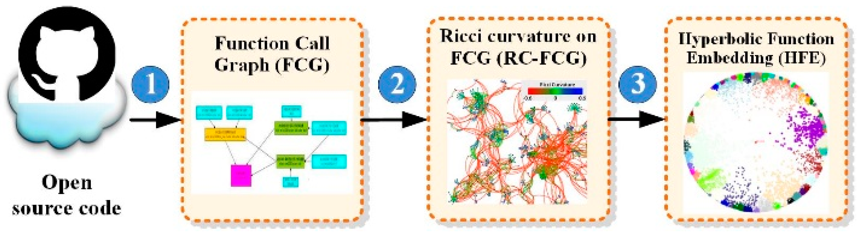
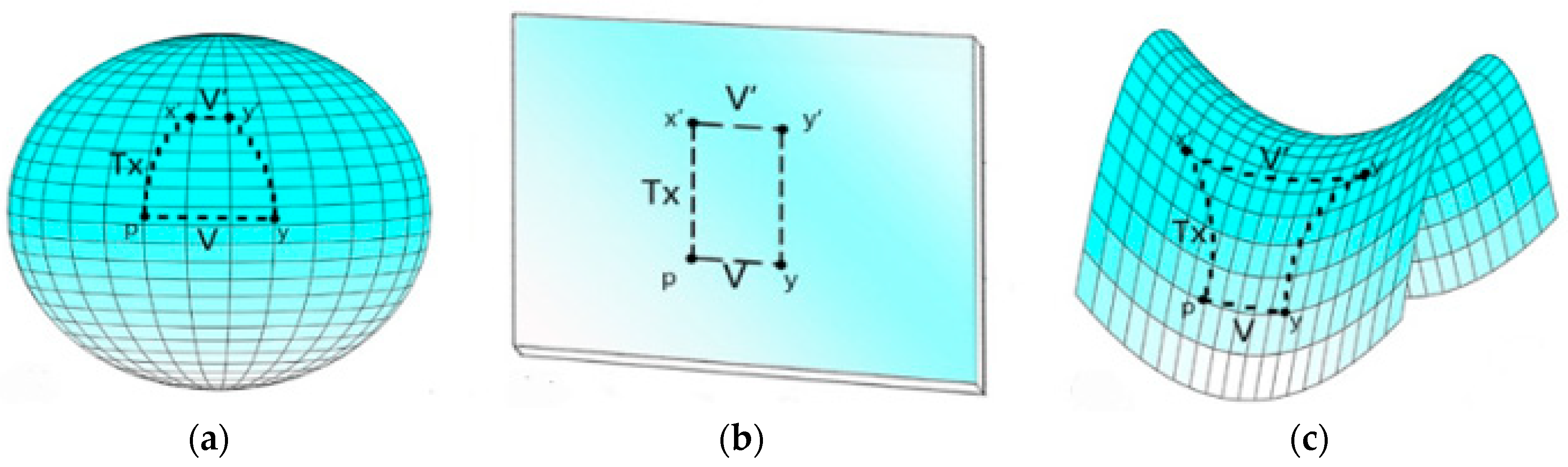
• We use Ricci curvature [15] to estimate the geometric structure of the FCG and identify that the curvature for most of the edges in the FCG are negative. This phenomenon suggests hyperbolic space instead of Euclidean space as a natural embedding space for FCG since hyperbolic space is usually associated with constant negative curvature [16]. Based on this observation, the original edge weights of the FCG are replaced by Ricci curvatures to form a new graph called RC-FCG, where the weight of each edge denotes the curvature from one node to the other node. The modified edge weights encode more information than the original edge weights.
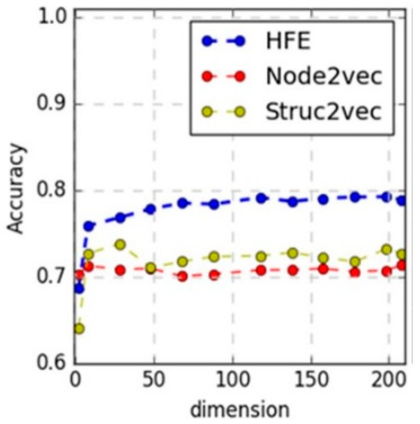
• Based on the RC-FCG, we propose a Poincaré disk-based hyperbolic function embedding (HFE) method to learn a hierarchical representation for RC-FCG in hyperbolic space. Our method achieves up to 7.6% performance improvement (especially in low-dimension situations) compared with the chosen state-of-the-art embedding methods, namely, Node2vec [17] and Struc2vec [18].

The rest of this paper is organized as follows: Section 2 describes the related works. The HFE model is discussed in Section 3. Section 4 provides experimental results and analysis. A summary of all the work of this study, together with the forecast for the further work, are given in Section 5.

2. Related Works

The successful application of a distributed representation [5] in NLP has inspired researchers to apply a distributed representation to source-code mining because of the naturalness hypothesis [5,19], which claimed that the statistical properties of source code are similar to those of natural language. Thus, most of the existing works that learn distributed representation from source code usually regarded a program as a bag of tokens [9] or a sequence of token [20,21]. Some of the existing works parsed the program to obtain the corresponding abstract syntax tree (AST) [10], which is suitable for tree-based neural networks, or extended an AST to a graph [22] for further processing. However, to the best of our knowledge, none of the existing work intended to learn the distributed representation from function-call graphs.

According to the underlying neural network models, the existing works can be generally classified as the following categories: forward neural network [9], recurrent neural network [10], convolutional neural network [20], auto-encoder [23], graph neural networks [24], etc. To the best of our knowledge, none of the existing works have ever analyzed the underlying geometric property of source code, established the connection between the hyperbolic space and the inherent hierarchy structure of source code, and applied distributed representation techniques for hyperbolic space, such as Poincaré embedding, to source code.

Although there were a few works that applied Poincaré embedding to NLP, the inherent differences between natural language and source code, such as formal syntax and semantics, which capture the most basic aspect of a program through function and function-call graph, make it difficult to directly apply the Poincaré embedding technique.

3. Hyperbolic Function Embedding

3.1. Overview

The proposed HFE framework includes three main steps, as shown in Figure 1:

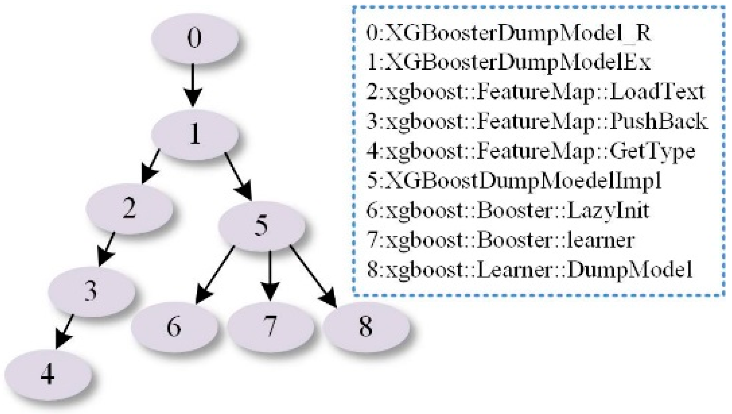
• Build a function call graph (FCG) from source code. Each node in the FCG denotes a function, and each edge in the FCG means a function-call relation. FCG can model the way in which a function is called in a context, i.e., a function-call semantic of code fragments (see Section 3.2 for more detail).
• Once the FCG is built, the Ricci curvature will be calculated for each pair of connected functions, and the calculated curvatures will replace the weight of each edge. The modified FCG is called RC-FCG. We believe that the Ricci curvature of each edge in the FCG carries much more information than the original one, and is suitable for hyperbolic space (see Section 3.3 for more detail).
• We learn a hyperbolic function embedding via the Poincaré ball model for RC-FCG (see Section 3.4 for more detail).

3.2. Function Call Graphs

An example of FCG is shown in Figure 2. Formally, $FCG=\left(F,CR\right)$ is a graph with a node set $F=\left\{f_1,f_2,\cdots ,f_n\right\}$ and an edge set $CR=\left\{c{r}_1,c{r}_2,\cdots ,c{r}_m\right\}$, where each node $f_i\in F,i=\left\{1,2,\cdots ,n\right\}$ denotes a function in the source code, and each edge $c{r}_l\in CR,l=\left\{1,2,\cdots ,m\right\}$ denotes a call relation between two functions. $FCG$ is a weighted graph where $w_{i,j}$ denotes the call frequency between $f_i$ and $f_j$. This call frequency describes the co-occurrence or call context of two functions, i.e., a call semantic. It is worth to note that for each individual program, the function-call edges in the FCG is deterministic. However, the proposed HFE method intends to learn the function-call statistics for all programs instead of an individual one. From the statistical point of view, each individual function may not be necessary. For example, modern programming frameworks, such as Android, iOS, and Panda, usually integrate a set of similar functions as a united API, which can be called in different ways based on the intended usage. Thus, for a large number of programs, whether a function is called, i.e., whether a function-call edge exists, can be regarded as a probabilistic distribution, which is the underlying reason that we use the call frequency as the edge weight.

The main processes are listed as follows:

Step 1.

The software tool Doxygen (http://www.stack.nl/~dimitri/doxygen/) is used to extract functions from source code. In this step, the name space is used to uniquely identify each function. Each function can be encoded by a hash function for tightening storage and fast search. Additionally, the other parts of the code, such as variable definition or assignment, can be mitted.

Step 2.

A sub-gragh is constructed for each function and the associated functions called inside. Then, the sub-graghs are merged into a larger graph called FCG. As mentioned before, the weight for each edge is the call frequency for two functions. We believe FCG can catch the call semantic relationship between functions.

Step 3.

Certain high-frequency functions, such as the set functions and the type-obtaining functions, are deleted to balance the global frequency of the whole graph.

3.3. FCG, Ricci Curvature, and Hyperbolic Space

In this section, we will analyze the fundamental property of the FCG from a geometric perspective, i.e., using Ricci curvature to determine the topological characteristics of the FCG. Ricci curvature can be an indicator to analyze the geometrical property of the FCG, which motivates us to adopt the Ricci curvature to replace the weights of the FCG and form a new graph called RC-FCG.

3.3.1. FCG and Ricci Curvature

We used the Ricci curvature to analyze the intrinsic geometric property of the FCG. The Ricci curvature [25] is a geometric local measure that can reflect intrinsic geometric property. This intrinsic attribute is fundamentally different from the other network metrics, such as degree, clustering coefficient, and betweenness centrality.

In this paper, we use the coarse Ricci curvature [15] to model the intrinsic geometric property of the FCG. Coarse Ricci curvature considers a metric space $\left(d,F\right)$ and a probability distribution $m_{f_i}$ on $F$, defined for each node $f_i$. The Ricci curvature $\kappa \left(f_i,f_j\right)$ for a pair of nodes $f_i,f_j\in F$ is obtained by comparing the Wasserstein distance from $m_{f_i}$ to $m_{f_j}$ and the distance $d\left(f_i,f_j\right)$.

In the FCG, the probability distribution $m_{f_i}$ for each function node $f_i\in F$ can be defined through Equation (1):

$$m_{f_i}\left(f_j\right)=\{\begin{array}{ll}\frac{w_{f_i,f_j}}{d_{f_i}},& \mathrm{if}{f}_j\sim f_i;\\ 0,& otherwise\end{array}$$

(1)

where $f_i\sim f_j$ represents nodes $f_i$ and $f_j$ are neighbors, $w_{f_i}{,}_{f_j}$ indicating the weight of the edge connecting $f_i$ and $f_j$, and $d_{f_i}$ represents the sum of the shortest distances from node $f_i$ to all of its neighboing nodes.

The Wasserstein distance from $m_{f_i}$ to $m_{f_j}$, denoted by $W\left(m_{f_i},m_{f_j}\right)$, is the minimum average traveling distance that can be achieved by Equation (2) [25,26,27]:

$$W\left(m_{f_i},m_{f_j}\right)=\underset{\xi }{\inf }{\displaystyle \sum _{f_i^{\prime },f_i^{\prime }\sim f_i}{\displaystyle \sum _{f_j^{\prime },f_j^{\prime }\sim f_j}d(}}{f}_i^{\prime },f_j^{\prime })\xi (f_i^{\prime },f_j^{\prime })$$

(2)

where $d\left(f_i^{\prime },f_j^{\prime }\right)$ is the length of the shortest path between $f_i^{\prime }$ and $f_j^{\prime }$, and $\xi (f_i^{\prime },f_j^{\prime })$ represents the mass moving from $f_i^{\prime }$ and $f_j^{\prime }$. It is worth noting that $\xi$ can be regarded as a transition matrix. The Wasserstein distance can be transformed to a linear programming (LP) problem via Kantorovich duality and computed effectively through linear programming (LP). For more information, one can refer to [28,29].

The coarse Ricci curvature $\kappa \left(f_i,f_j\right)$ for two functions in the FCG can be calculated by the Wasserstein distance from $m_{f_i}$ to $m_{f_j}$ and distance $d\left(f_i,f_j\right)$, as shown in Equation (3):

$$\kappa \left(f_i,f_j\right)=1-\frac{W\left(m_{f_i},m_{f_j}\right)}{d\left(f_i,f_j\right)}$$

(3)

Using Equation (3), we can re-calculate weights of FCG according to Ricci curvature, as shown in Equation (4):

$$w_{f_i,f_j}=normalized\left(\kappa \left(f_i,f_j\right)\right)$$

(4)

Since the Ricci curvature can be negative, we normalized it from 0 to 1.

3.3.2. RC-FCG and Hyperbolic Space

Figure 3 intuitively illustrates the relation between curvature and space, where positive, zero, and negative curvatures correspond to spherical, Euclidean, and hyperbolic spaces, respectively. Intuitively, the correspondence between Ricci curvature and the geometry space can be illustrated as follows. In Figure 3a–c, $p$ is a point on the corresponding manifold $M$ in spherical, Euclidean, and hyperbolic spaces, respectively. At point $p$, two orthogonal tangent vectors $T_x$ and V intersect with $M$ at points $x^{\prime }$ and $y$, respectively. At point $y$, a tangent vector that is orthogonal to $V$ intersects with $M$ at point $y^{\prime }$. If the length of the tangent vector $V^{\prime }$ that connects $x^{\prime }$ and $y^{\prime }$, and is orthogonal to $T_x$ and $y$, $y^{\prime }$, is shorter than $V$, the corresponding manifold is related to spherical space, as shown in Figure 3a. Otherwise, if the length of the tangent vector $V^{\prime }$ is larger than $V$, the corresponding manifold is related to hyperbolic space, as shown in Figure 3c. Otherwise, the corresponding manifold is related to Euclidean space, as shown in Figure 3b. In the discrete cases, the Ricci curvature of each edge in a square lattice graph is equal to zero, the Ricci curvature of each edge in a tree or hierarchy structure is negative except the ones connecting leaf nodes, and the Ricci curvature of each edge in a complete graph is positive.

Figure 4 shows the distribution of Ricci curvature of a generated FCG with 34,987 edges in total, where 23,241 edges have negative Ricci curvature. The proportion is about 2/3. This result suggests that hyperbolic space is the underlying geometry of the FCG. Thus, it may be a good choice to model the FCG in hyperbolic space.

3.4. Learning HFE via the Poincaré Ball Model

3.4.1. Hyperbolic Space and the Poincaré Ball Model

Since the function-call relations in source code are organized in a hierarchical way and the distribution of negative Ricci curvature of the FCG is dominating, as illustrated in Figure 4, it inspires us to design a representation for the RC-FCG in hyperbolic space, which can be used to model hierarchical structures. Since the RC-FCG is hierarchical in nature, it is straightforward to learn a representation for the RC-FCG in hyperbolic space in order to preserve hierarchical structures.

There are several important models of hyperbolic space: the Klein model, the hyperboloid model, the Poincaré ball model, and the Poincaré half space model [30]. Inspired by Poincaré embedding, we use the Poincaré ball model for the convenience of gradient-based optimization.

3.4.2. Hyperbolic Distance for the Poincaré Ball Model

Formally, let ${\mathcal{B}}^d=\left\{\mathit{x}\in R^d|\Vert \mathit{x}\Vert <1\right\}$ with $\Vert .\Vert$ as the Euclidean norm be the open d-dimensional unit ball. The Poincaré ball model corresponds to the Riemannian manifold $\left({\mathcal{B}}^d,g_x\right)$. The Riemannian metric tensor defined on ${\mathcal{B}}^d$ can be written as follows:

$$g_x={\left(\frac{2}{1-{\Vert \mathit{x}\Vert }^2}\right)}^2{g}^E$$

(5)

where $\mathit{x}\in {\mathcal{B}}^d$ and $g^E$ is the Euclidean metric tensor. Under ${\mathcal{B}}^d$, the hyperbolic distance for Poincaré ball can be defined as follows.

$$d_h\left(\mathit{u},\mathit{v}\right)=arcosh\left(1+2\frac{\Vert \mathit{u}-\mathit{v}\Vert }{\left(1-{\Vert \mathit{u}\Vert }^2\right)\left(1-{\Vert \mathit{v}\Vert }^2\right)}\right)\mathit{u},\mathit{v}\in {\mathcal{B}}^d$$

(6)

where $arcosh\left(\mathit{u}\right)=\ln \left(\mathit{u}+\sqrt{{\mathit{u}}^2-1}\right)$ is the inverse hyperbolic cosine function. The $d_h\left(\mathit{u},\mathit{v}\right)$ in hyperbolic space is able to discover the underlying hierarchy structure according to the representation coordination of functions in the Poincaré ball model. Based on Equation (6), the hyperbolic distance will exponentially increase along with the vector’s norm approximating 1. From a visual view, the origin of the Poincaré ball can be regarded as the root of a tree, the branches or leaves of which extend toward the boundaries of the Poincaré ball, where the hyperbolic distance grows exponentially. Thus, the potential hierarchies of the $RC-FCG$ are captured. The visualization analysis will be presented in Section 4.3.

3.4.3. Loss Function and Optimization

For a set of functions $F={\left\{f_i\right\}}_{i=1}^n$, to train the corresponding HFE vectors $\mathrm{\Theta }={\left\{{\mathit{\theta }}_i\right\}}_{i=1}^n$, where ${\mathit{\theta }}_i\in {\mathcal{B}}^d$, a loss function $\mathcal{L}\left(\mathrm{\Theta }\right)$ is proposed, as shown in Equation (7), which is inspired by word2vec [5]:

$$\mathcal{L}\left(\mathrm{\Theta }\right)={\displaystyle \sum _{f_i,f_j\in CR}\log \frac{e^{-d\left({\mathit{\theta }}_{fi},{\mathit{\theta }}_{f_j}\right)}}{{\displaystyle {\sum }_{f_j^{\prime }\in N\left(f_i\right)}{e}^{-d\left({\mathit{\theta }}_{fi},{\mathit{\theta }}_{f_j^{\prime }}\right)}}}}$$

(7)

where $N\left(f_i\right)=\left\{f_j|\left(f_i,f_j\right)\notin CR\right\}\cup \left\{f_i\right\}$ is the set of negative samples for $f_i$, ${\mathit{\theta }}_{f_i}$ represents an embedding vector corresponding to function $f_i$ in ${\mathcal{B}}^d$, and $d({\theta }_{f_i},{\theta }_{f_j})$ denotes the hyperbolic distance between the two embedding vectors ${\theta }_{f_i}$ and ${\theta }_{f_j}$. From Equation (7), it can be inferred that, to minimize the loss function, the hyperbolic distance between a pair of connected functions in the FCG is forced to be reduced, while the hyperbolic distance between any disconnected functions is forced to be enlarged. Therefore, the loss function $\mathcal{L}\left(\mathrm{\Theta }\right)$ can help HFE preserve the edge information of the FCG.

In hyperbolic space, parameters are learned via stochastic Riemannian optimization methods, such as RSGD [31,32]. In particular, let ${{\rm T}}_{\theta }\mathcal{B}$ denote the tangent space of a point $\mathit{\theta }\in {\mathcal{B}}^d$. Furthermore, let ${\nabla }_R\in {{\rm T}}_{\theta }\mathcal{B}$ and ${\nabla }_E$ denote the Riemannian gradient and Euclidean gradient of $\mathcal{L}\left(\mathsf{\Theta }\right)$, respectively. The parameters in RSGD can be updated based on Equation (8):

$${\mathit{\theta }}_{t+1}=R_{{\theta }_t}\left(-\eta {\nabla }_R\mathcal{L}\left({\mathit{\theta }}_t\right)\right)$$

(8)

where $R_{{\theta }_t}$ means retraction onto $\mathcal{B}$ at ${\mathit{\theta }}_t$, $\eta$ is the learning rate at step $t$. In practice, the Riemannian gradient ${\nabla }_R$ can be derived from the Euclidean gradient ${\nabla }_E$. Specifically, the Euclidean gradient is as follows:

$${\nabla }_E=\frac{\partial \mathcal{L}({\theta }_{fi})}{\partial d({\theta }_{f_i},{\theta }_{f_j})}\frac{\partial d({\theta }_{f_i},{\theta }_{f_j})}{\partial {\theta }_{f_i}}$$

(9)

where L(${\mathit{\theta }}_{f_i}$) is the part of the total loss $\mathcal{L}\left(\mathrm{\Theta }\right)$ that relates to function $f_i$, as shown in Equation (10):

$$\mathcal{L}\left({\theta }_{f_i}\right)={\displaystyle \sum _{f_i\sim f_j}\log \frac{e^{-d\left({\mathit{\theta }}_{fi},{\mathit{\theta }}_{f_j}\right)}}{{\displaystyle {\sum }_{f_j^{\prime }\in N\left(f_i\right)}{e}^{-d\left({\mathit{\theta }}_{f_i},{\mathit{\theta }}_{f_j^{\prime }}\right)}}}}$$

(10)

Based on Equation (10), it can easily derive the first partial derivative in Equation (9), and based on Equation (6), we can also compute the second partial derivate in Equation (9). Combining with Equation (5), we can derive the correspondence between the Riemannian gradient and the Euclidean gradient [33], as shown in Equation (11):

$${\nabla }_R=\frac{{(1-{\Vert {\mathit{\theta }}_t\Vert }^2)}^2}{4}{\nabla }_E$$

(11)

Furthermore, in order to map the learned embeddings into the Poincaré ball model, the following mapping operations are adopted:

$$map(\mathit{\theta })=\{\begin{array}{ll}\mathit{\theta }/\Vert \mathit{\theta }\Vert -\delta ,& if\Vert \mathit{\theta }\Vert \ge 1\\ \mathit{\theta },& otherwise\end{array}$$

(12)

where $\delta$ is a small constant, set as ${10}^{-7}$. In a word, the update for a single embedding is of the form as shown in Equation (13):

$${\mathit{\theta }}_{t+1}\leftarrow map({\mathit{\theta }}_t-{\eta }_t\frac{{(1-{\Vert {\mathit{\theta }}_t\Vert }^2)}^2}{4}{\nabla }_E)$$

(13)

4. Experiments and Analysis

In this section, we evaluate the performance of the HFE for two application scenarios: function clustering and link (i.e., function-call relation) prediction.

4.1. Dataset and Baseline

4.1.1. Dataset

The experiments datasets are the top 10 C++ open-sourced software collected from Github. A program parser tool named Doxygen has been applied to those source codes to extract the functions and their call relations. Using method mentioned in the Section 3.1, the corresponding FCG and RC-FCG are built. Once the RC-FCG is built, it will be fed into the HFE model to learn an HFE vector for each individual function. Since the RC-FCG consists of a random forest, instead of a tree, it is desirable to merge the forest into a connected graph. To achieve this, a virtual root node is introduced as the virtual parent node of all the root nodes of the trees in the forest. Note that the introduced virtual node is also the center of the Poincaré ball model. Additionally, the isolated functions, which do not to connect other functions in the RC-FCG, are removed from the connected graph. In total, the final RC-FCG has 16,170 vertices (functions) and 248,118 edges (function-call relations).

4.1.2. Baselines

Two state-of-the-art embedding models, namely, Node2vec [17] and Struct2vec [18], are selected as baselines for evaluating the HFE’s performance. Node2vec designed a two-order random walk with two parameters to control the tradeoff between depth first search (DFS) and breadth first search (BFS). In our contrastive experiments, the parameters of Node2vec are set to prefer BFS, while the parameters of Struc2vec are set to the default values.

In the experiments, Riemannian gradient descent of HFE is used to update the parameters with the initial learning rate being 0.1, the final learning rate being 0.0001, and the training epoch being 10.

4.2. Performance Comparison and Analysis

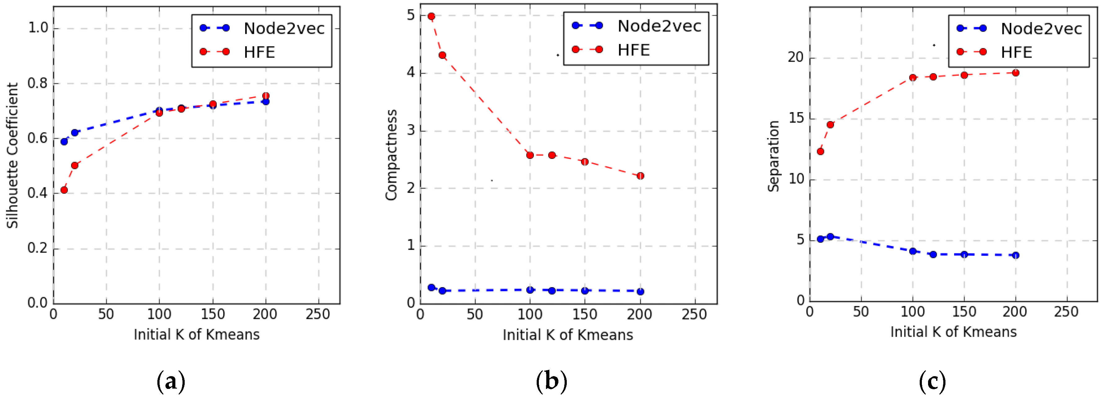
4.2.1. Clustering

One prominent advantage of HFE is its capability to simultaneously capture function similarity and function hierarchy information in a continuous vector space. To illustrate these experiments have been conducted to cluster the functions via the k-means clustering algorithm based on the vectors learned through the HFE and Node2vec, respectively. Since the distance metric among distributed vectors usually reflects the semantic similarity among them, it is likely that functions with semantic and/or similar hierarchy levels may appear in the same cluster.

In order to evaluate the effect of clustering, we adopt three representative criteria: (1) Compactness (CP), which is defined as the average distance from a data point of a cluster to the cluster center; (2) degree of separation (SP), which denotes the average distance between any two- cluster center; and (3) silhouette coefficient (SC), which evaluates the clustering performance through the ratio of CP to SP. A good cluster result should satisfy the following criteria: (1) SC approaching 1 asynchronously, (2) smaller CP, (3) larger SP, and (4) an appropriate value of k.

Figure 5 shows the performance trend of the above three metrics along with the variation of k, in a low embedding dimension (d = 2). From Figure 5a, it can be observed that the SC of HFE is higher than that of Node2vec when k is larger than 120. From Figure 5c, it can be concluded that the SP of HFE is much higher than that of Node2vec. However, from Figure 5b, it can be revealed that the CP of Node2vec is better instead. This is because HFE needs to consider not only semantic similarity, but also hierarchical similarity. For example, semantically similar functions may appear in different hierarchical levels, which denote a larger distance than the case without considering hierarchy information. This phenomenon is consistent with the fact that the hyperbolic space is usually larger than the Euclidean space, which implies that both inter-cluster distance and intra-cluster distance are larger in hyperbolic space. Moreover, along with the increment of the cluster number, the inter-cluster distance and intra-cluster distance associated with HFE significantly increase and decrease, respectively, while those two distances associated with Node2vec only show small variation. This reflects that HFE is much more sensitive to the variation of the cluster number. The underlying reason may lie in that HFE can take advantage of the hierarchy information embedded in the larger hyperbolic space to cluster functions more precisely and accurately. Thus, HFE is better than Node2vec when the cluster number k is larger than 120, as shown in Figure 5a. The similar phenomenon can also be found in traffic networks [33].

To intuitively apprehend the hierarchy property, both the embedding vectors generated from HFE and Node2vec are visualized by adopting different colors and symbols to denote different clusters, as shown in Figure 6a,c respectively. In Figure 6a, the distribution of HFE is visualized through the Poincaré disk model, which reveals a prominent hierarchical structure from the FCG virtual root in the disk center to the FCG leaves around the disk boundary. However, the distribution of Node2vec shown in Figure 6c does not reveal the hierarchical structure.

To illustrate that HFE captures semantic similarity, we extract a subtree with 50 functions and 78 edges, and embed the tree through HFE (shown in Figure 6b) and Node2vec (shown in Figure 6d), respectively. From these figures it can be concluded that both HFE and Node2vec reveal semantic similarity because similar functions are closer to each other. However, HFE also shows a hierarchical structure, which is not learned by Node2vec in Euclidean space.

4.2.2. Link Prediction

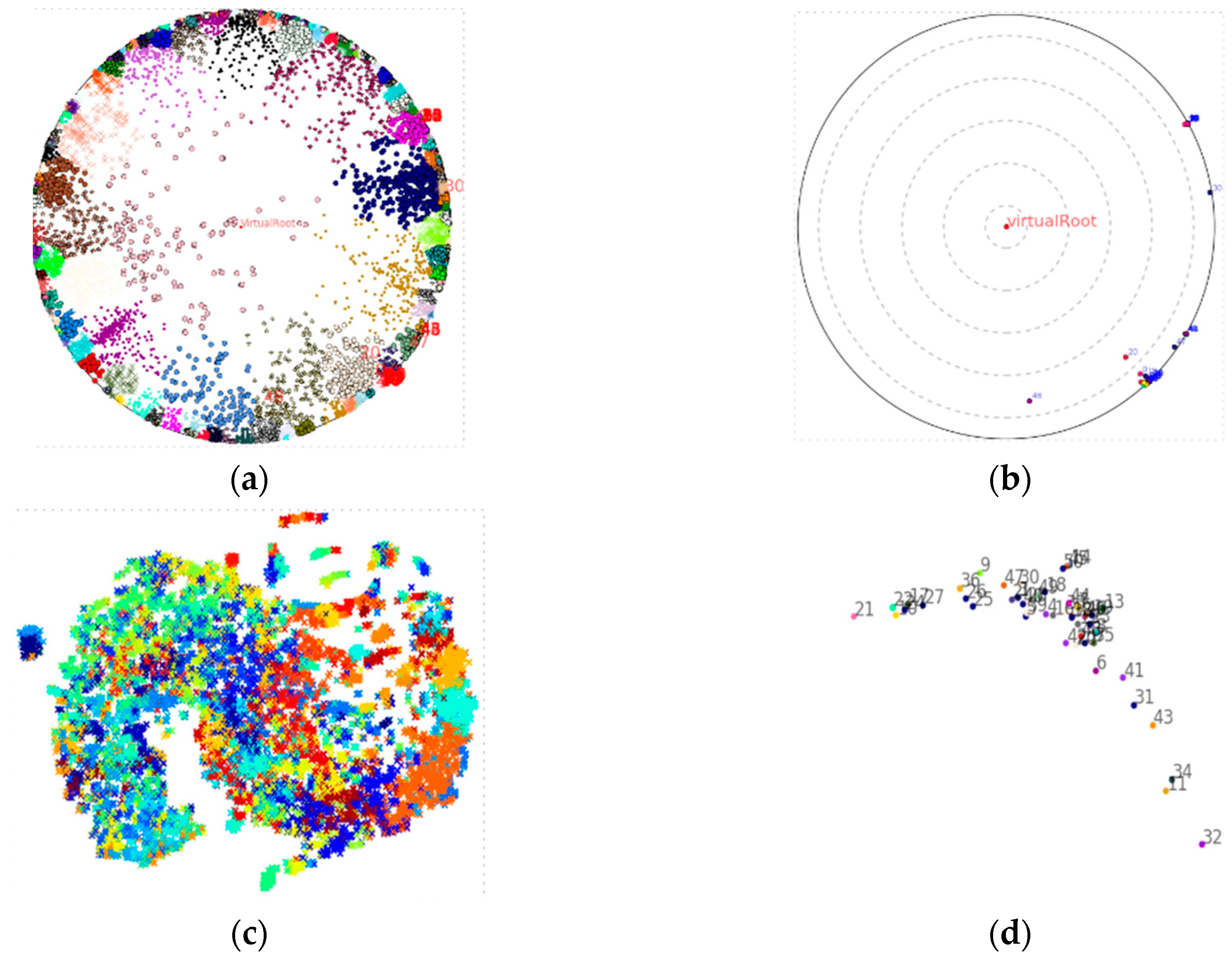
In the link prediction scenarios, the goal is to predict whether a function-call relation exists between two function nodes. This application scenario can reveal whether the HFE learn the structural information implied in the function-call relations. We randomly hide 10% of edges in the original RC-FCG as positive ground truth, then use the rest of the edges to train models, such as Struc2vec, Node2vec, and HFE. After training, we obtain the representation vectors for all functions and then use logistic regression to predict the probability of edge existence for a given function node pair. The test set consists of positive samples and negative samples with equal number. The former includes the hidden 10% vertex pairs mentioned above in the original RC-FCG, while the latter is made up of randomly chosen disconnected vertex pairs.

The accuracy results are shown in Figure 7, which shows that HFE outperforms all the baselines. Specifically, when the space dimension is eight dimensions (i.e., low dimension), HFE improves 2.5% and 4.7% in terms of accuracy compared with Struc2vec and Node2vec, respectively. When the space dimension is 208 dimensions (i.e., high dimension), HFE improves 6.2% and 7.6% in terms of accuracy compared with Struc2vec and Node2vec, respectively, as shown in

Table 1. The accuracy of three models varying with dimension.

Model	RC-FCG
	Accuracy
	8-dim	2018-dim
Node2vec	0.7047	0.7131
Struc2vec	0.7269	0.7271
HFE	0.7519	0.7891

. Furthermore, it can be observed from Figure 7 that HFE can achieve a better performance with a low-dimension space (eight dimensions) representation than all baseline methods with a high-dimension space (208 dimensions). This observation reflects that HFE can learn the function-call relations better even with smaller space dimension, i.e., HFE can learn a more compact representation without performance loss. The underlying reason may lie in that the volume in hyperbolic space grows exponentially, while the volume of Euclidean space expands only polynomially. Thus, the learned representation embedded in hyperbolic space may have higher capacity that those in Euclidean space [34,35].

4.3. Visualization

In this section, we visualize an example to illustrate the way by which HFE learn the function-call hierarchical structure. We extract a subtree, named the phone numbers tree (PNT), as shown in Figure 8a, from the entire FCG. In Figure 8b, the learned HFE corresponding to the PNT subtree is visualized in the Poincaré disk. It is worthy to note that, to compare the PNT subtree and the corresponding HFE, the same number and the same color are used to identify the same function and the same function-call path from the root to the leaf in both Figure 8a,b, respectively. For example, paths 1->2->23->37 in both Figure 8a,b is green. Notably, in Figure 8b, the hierarchy is reflected by the concentric circles.

Considering the path $1\to 2\to 23\to 37$ in the PNT, node 1 represents function testVoip(), which is designed to check whether a phone number is valid. Nodes 2, 23, and 37 denote functions checkNumbersValidAndCorrecttype(),isValidNumber(),andisValidNumberForRegion(),respectively. Figure 8b shows that nodes 1, 2, 23, and 37 lie on different concentric circles from the root (center) to the margin (leaf). Moreover, node 2 lies on the concentric circle other than nodes 20–22. The underlying reason may lie in that node 2 has a larger subtree, which usually corresponds to smaller curvature. Hence, in Figure 8b, node 2 should be farther from the root than nodes 20–22, even though those four nodes are at the same level in the PNT tree. From this example, we can see that HFE indeed learns the hierarchical structure of the FCG.

5. Conclusions and Future Works

In this paper, we propose a novel hyperbolic function embedding method, which can learn a distributed and hierarchical representation for each function via the Poincaré ball model. The proposed method builds a function-call graph to model the function-call relations or function-call context for each function. Within the FCG, the function’s semantic is encoded in the neighborhood of a node. We also use the Ricci curvature to describe the intrinsic geometry of the FCG. We find that the negative Ricci curvature of the edges in the FCG is dominant, which motivates us to represent functions in a hyperbolic instead of Euclidean space. We also build an RC-FCG by replacing the edge weight in the FCG with the corresponding Ricci curvature. The RC-FCG encodes richer topologic information than the FCG. Finally, an HFE model is built to learn a representation of the RC-FCG. The HFE can capture the latent hierarchy of functions in the hyperbolic space, which is very important to learn a representation model for function analysis since functions in source code are naturally organized in a hierarchical way. Experiments show that HFE achieves up to 7.6% performance improvement compared to the chosen state-of-the-art graph embedding methods. In the future, we will further explore the geometric property of the RC-FCG because we believe that the intrinsic geometry encoded via Ricci curvature of the RC-FCG is critical, which needs further theoretical explanation.

References

1. Allamanis, M.; Barr, E.T.; Devanbu, P.; Sutton, C. A Survey of Machine Learning for Big Code and Naturalness. ACM Comput. Surv. 2018, 51, 1–37. [Google Scholar] [CrossRef]
2. Gupta, R.; Pal, S.; Kanade, A.; Shevade, S. DeepFix: Fixing Common C Language Errors by Deep Learning. In Proceedings of the AAAI, San Francisco, CA, USA, 4–9 February 2017; pp. 1345–1351. [Google Scholar]
3. Hu, X.; Wei, Y.; Li, G.; Jin, Z. CodeSum: Translate Program Language to Natural Language. arXiv, 2017; arXiv:1708.01837. [Google Scholar]
4. Knuth, D.E. Literate Programming. Comput. J. 1984, 27, 97–111. [Google Scholar] [CrossRef] [Green Version]
5. Mikolov, T.; Sutskever, I.; Chen, K.; Corrado, G.S.; Dean, J. Distributed representations of words and phrases and their compositionality. Adv. Neural Inf. Process. Syst. 2013, 26, 3111–3119. [Google Scholar]
6. Gu, X.; Zhang, H.; Zhang, D.; Kim, S. Deep API Learning. In Proceedings of the 2016 24th ACM SIGSOFT International Symposium on Foundations of Software Engineering 2016, Seattle, WA, USA, 13–19 November 2016. [Google Scholar]
7. Iyer, S.; Konstas, I.; Cheung, A.; Zettlemoyer, L. Summarizing source code using a neural attention model. In Proceedings of the 54th Annual Meeting of the Association for Computational Linguistics, Berlin, Germany, 7–12 August 2016; pp. 2073–2083. [Google Scholar]
8. Piech, C.; Huang, J.; Nguyen, A.; Phulsuksombati, M.; Sahami, M.; Guibas, L. Learning Program Embeddings to Propagate Feedback on Student Code. arXiv, 2015; arXiv:1505.05969. [Google Scholar]
9. Nguyen, T.D.; Nguyen, A.T.; Phan, H.D.; Nguyen, T.N. Exploring API Embedding for API Usages and Applications. In Proceedings of the 2017 IEEE/ACM 39th International Conference on Software Engineering (ICSE), Buenos Aires, Argentina, 20–28 May 2017. [Google Scholar]
10. Mou, L.; Li, G.; Zhang, L.; Wang, T.; Jin, Z. Convolutional Neural Networks over Tree Structures for Programming Language Processing. In Proceedings of the AAAI, Québec City, QC, Canada, 27–31 July 2014. [Google Scholar]
11. Chamberlain, B.P.; Clough, J.; Deisenroth, M.P. Neural Embeddings of Graphs in Hyperbolic Space. arXiv, 2017; arXiv:1705.10359. [Google Scholar]
12. Krioukov, D.; Papadopoulos, F.; Kitsak, M.; Vahdat, A.; Boguná, M. Hyperbolic Geometry of Complex Networks. Phys. Rev. E Stat. Nonlinear Soft Matter Phys. 2010, 82, 036106. [Google Scholar] [CrossRef] [PubMed]
13. Verbeek, K.; Suri, S. Metric Embedding, Hyperbolic Space, and Social Networks; Elsevier Science Publishers, B.V.: Amsterdam, The Netherlands, 2016. [Google Scholar]
14. Nickel, M.; Kiela, D. Poincaré Embeddings for Learning Hierarchical Representations. In Proceedings of the Advances in Neural Information Processing Systems, Long Beach, CA, USA, 4–9 December 2017. [Google Scholar]
15. Lohkamp, J. Metrics of Negative Ricci Curvature. Ann. Math. 1994, 140, 655–683. [Google Scholar] [CrossRef]
16. Ollivier, Y. Ricci curvature of Markov chains on metric spaces. J. Funct. Anal. 2009, 256, 810–864. [Google Scholar] [CrossRef] [Green Version]
17. Grover, A.; Leskovec, J. Node2vec: Scalable Feature Learning for Networks. In Proceedings of the ACM Sigkdd International Conference on Knowledge Discovery & Data Mining, San Francisco, CA, USA, 13–17 August 2016. [Google Scholar]
18. Ribeiro, L.F.R.; Saverese, P.H.P.; Figueiredo, D.R. Struc2vec: Learning Node Representations from Structural Identity. In Proceedings of the 23rd ACM SIGKDD International Conference on Knowledge Discovery and Data Mining, Halifax, NS, Canada, 13–17 August 2017. [Google Scholar]
19. Vilnis, L.; Mccallum, A. Word Representations via Gaussian Embedding. arXiv, 2014; arXiv:1412.6623. [Google Scholar]
20. Allamanis, M.; Peng, H.; Sutton, C. A Convolutional Attention Network for Extreme Summarization of Source Code. In Proceedings of the International Conference on Machine Learning, New York City, NY, USA, 19–24 June 2016. [Google Scholar]
21. Dam, H.K.; Tran, T.; Pham, T.T.M. A deep language model for software code. arXiv, 2016; arXiv:1608.02715. [Google Scholar]
22. Allamanis, M.; Brockschmidt, M.; Khademi, M. Learning to Represent Programs with Graphs. arXiv, 2017; arXiv:1711.00740. [Google Scholar]
23. Allamanis, M.; Chanthirasegaran, P.; Kohli, P.; Sutton, C. Learning Continuous Semantic Representations of Symbolic Expressions. In Proceedings of the 34th International Conference on Machine Learning, Sydney, Australia, 6–11 August 2017. [Google Scholar]
24. Li, Y.; Tarlow, D.; Brockschmidt, M.; Zemel, R. Gated Graph Sequence Neural Networks. arXiv, 2015; arXiv:1511.05493. [Google Scholar]
25. Jürgen, J.; Liu, S. Ollivier’s Ricci Curvature, Local Clustering and Curvature-Dimension Inequalities on Graphs. Discr. Comput. Geometry 2014, 51, 300–322. [Google Scholar] [CrossRef]
26. Villani, C. Optimal Transport. Grundlehren Der Mathematischen Wissenschaften. In The Analysis of Linear Partial Differential Operators; Springer: New York, NY, USA, 2009. [Google Scholar]
27. Ollivier, Y.; Villani, C. A Curved Brunn--Minkowski Inequality on the Discrete Hypercube, Or: What Is the Ricci Curvature of the Discrete Hypercube? SIAM J. Discr. Math. 2012, 26, 983–996. [Google Scholar] [CrossRef] [Green Version]
28. Shi, J.; Zhang, W.; Wang, Y. Shape Analysis with Hyperbolic Wasserstein Distance. In Proceedings of the 2016 IEEE Conference on Computer Vision and Pattern Recognition (CVPR), Las Vegas, NV, USA, 27–30 June 2016. [Google Scholar]
29. Santambrogio, F. Optimal transport for applied mathematicians. In Progress in Nonlinear Differential Equations & Their Applications; Springer: Birkäuser, NY, USA, 2015; pp. 99–102. [Google Scholar]
30. Gromov, M. Hyperbolic groups. In Essays in Group Theory; Springer: New York, NY, USA, 1987. [Google Scholar]
31. Zhang, H.; Reddi, S.J.; Sra, S. Riemannian SVRG: Fast Stochastic Optimization on Riemannian Manifolds. In Proceedings of the Advances in Neural Information Processing Systems, Barcelona, Spain, 5–10 December 2016. [Google Scholar]
32. Bonnabel, S. Stochastic Gradient Descent on Riemannian Manifolds. IEEE Trans. Autom. Control 2013, 58, 2217–2229. [Google Scholar] [CrossRef] [Green Version]
33. Jonckheere, E.; Lou, M.; Bonahon, F.; Baryshnikov, Y. Euclidean versus Hyperbolic Congestion in Idealized versus Experimental Networks. Internet Math. 2011, 7, 1–27. [Google Scholar] [CrossRef] [Green Version]
34. Wang, C.; Jonckheere, E.; Brun, T. Differential geometric treewidth estimation in adiabatic quantum computation. Quant. Inf. Process. 2016, 15, 3951–3966. [Google Scholar] [CrossRef]
35. Gulcehre, C.; Denil, M.; Malinowski, M.; Razavi, A.; Pascanu, R.; Hermann, K.M.; Battaglia, P.; Bapst, V.; Raposo, D.; Santoro, A.; et al. Hyperbolic Attention Networks. arXiv, 2010; arXiv:1805.09786. [Google Scholar]
Figure 1. Overview of proposed HFE framework.
Symmetry 11 00254 g001
Figure 2. The illustration of the hierarchical structure of the function call from boost library (http://www.boost.org/).
Symmetry 11 00254 g002
Figure 3. Curvature and space. (a) Positive curvature implies spherical space; (b) zero curvature implies plane Euclidean space; and (c) negative curvature implies hyperbolic space.
Symmetry 11 00254 g003
Figure 4. The density distribution of Ricci curvature on a FCG.
Symmetry 11 00254 g004
Figure 5. The variations of the three clustering performance metrics along with the variations of k. (a) SC; (b) CP; (c). SP.
Symmetry 11 00254 g005
Figure 6. Two-dimensional function embeddings are clustered in different space: (a) in hyperbolic space; (b) subtree in hyperbolic space; (c) in Euclidean space. Each color or symbol denotes one clustering class, Moreover, the embeddings in identical color or closer distance are similar.; (d) subtree in Euclidean space.
Symmetry 11 00254 g006
Figure 7. The accuracy of the three models varying with dimension.
Symmetry 11 00254 g007
Figure 8. The PNT subtree and the visualization of the corresponding two-dimensional HFE. (a) A subtree of PNT; (b) The project of Poincaré disk of above subtree of PNT.
Symmetry 11 00254 g008