Parametric Fault Diagnosis of Analog Circuits Based on a Semi-Supervised Algorithm


Abstract
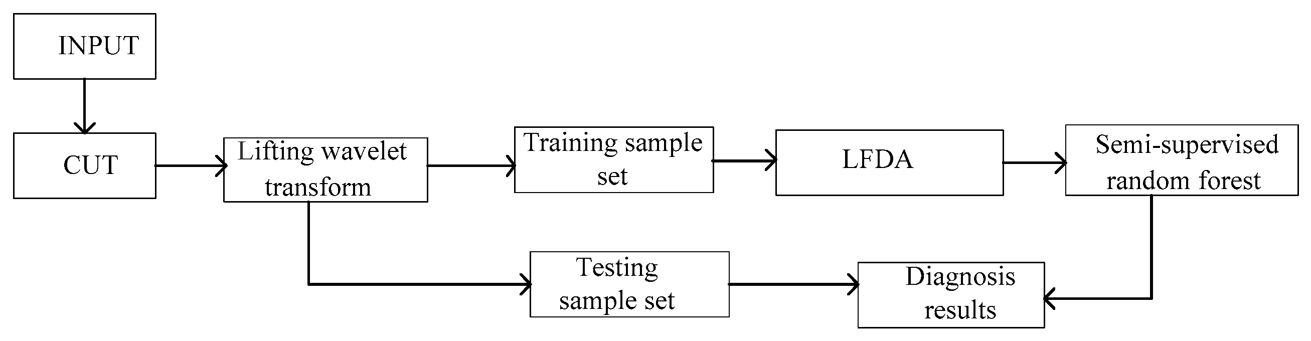
:1. Introduction
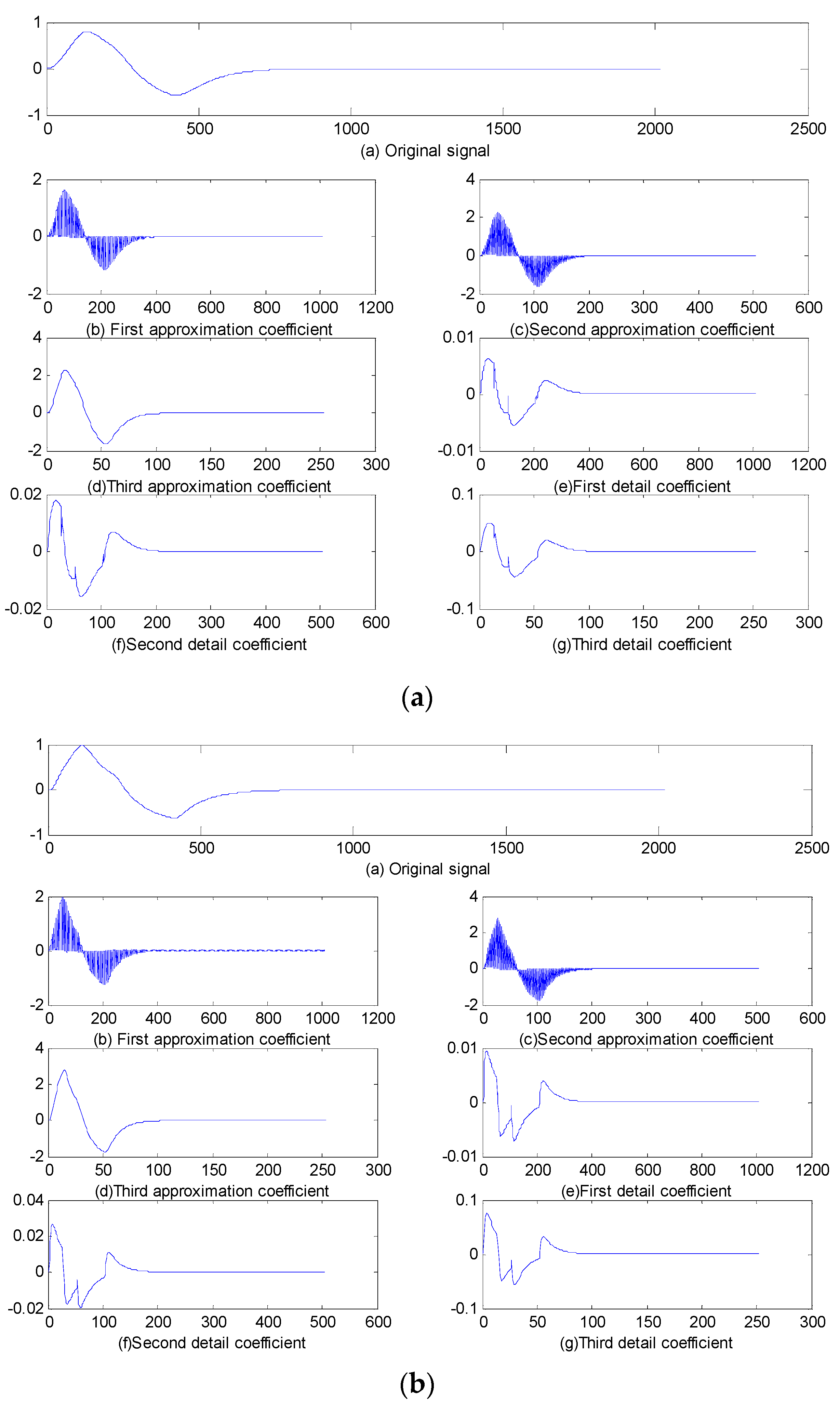
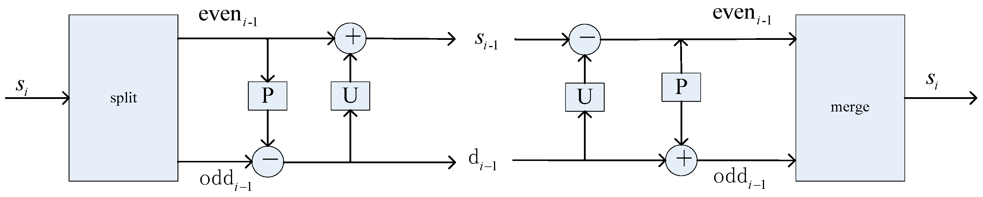
2. Lifting Wavelet Transform
3. Local Fisher Discriminant Analysis (LFDA)
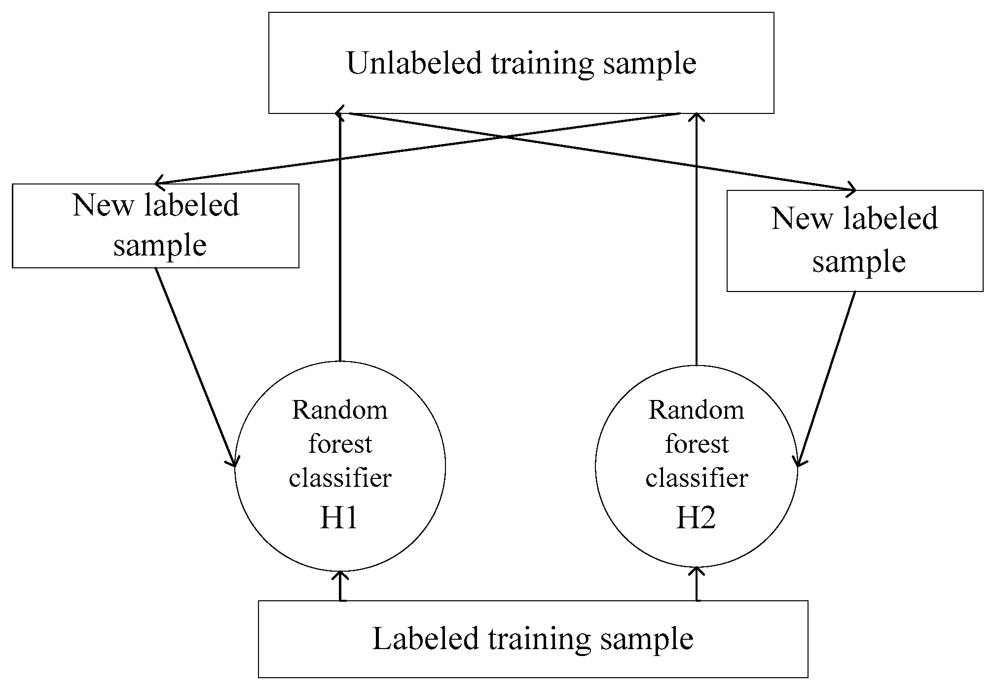
4. Semi-Supervised Random Forest Algorithm
5. Experimental Results and Discussion
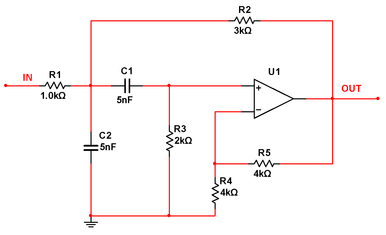
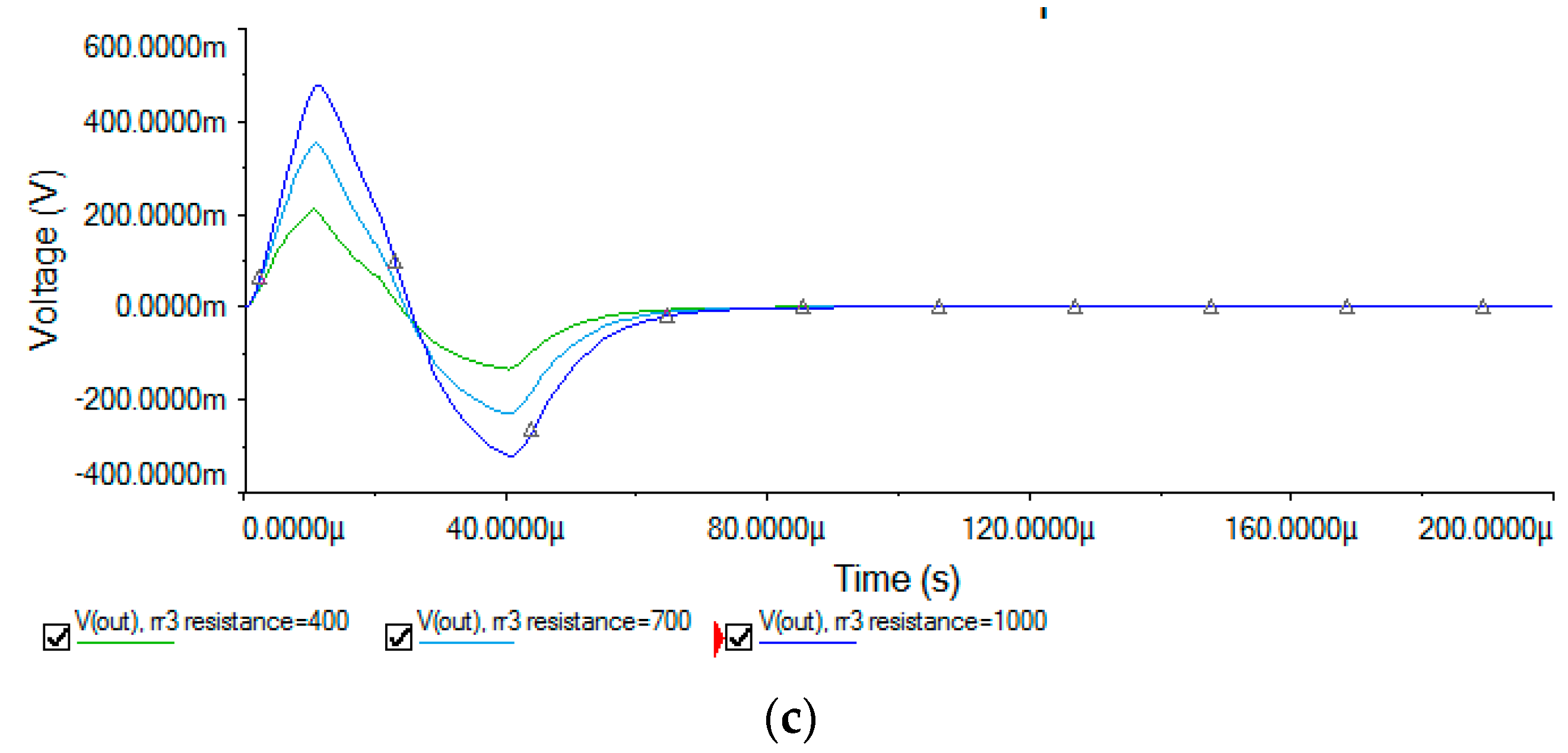
5.1. Sallen–Key Band-Pass Filter Circuit
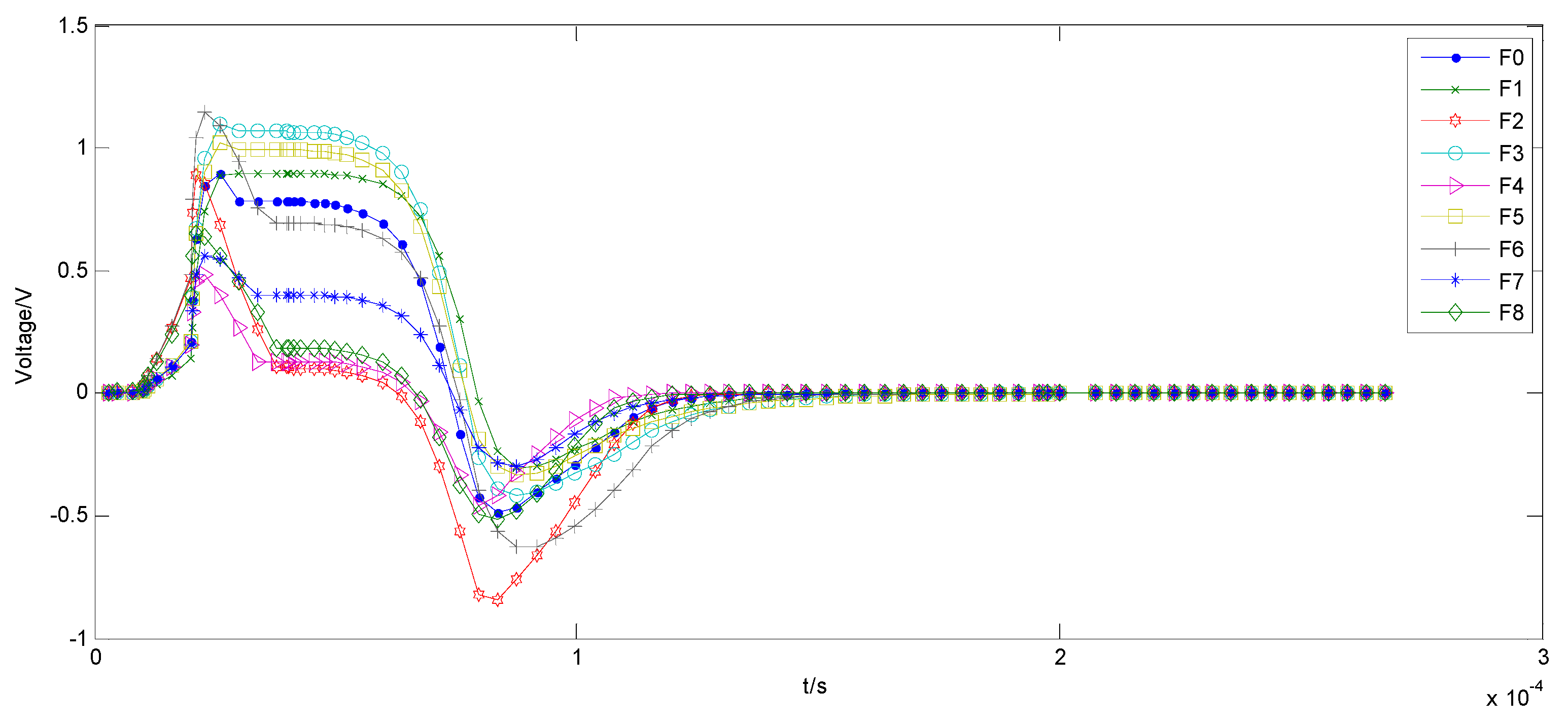
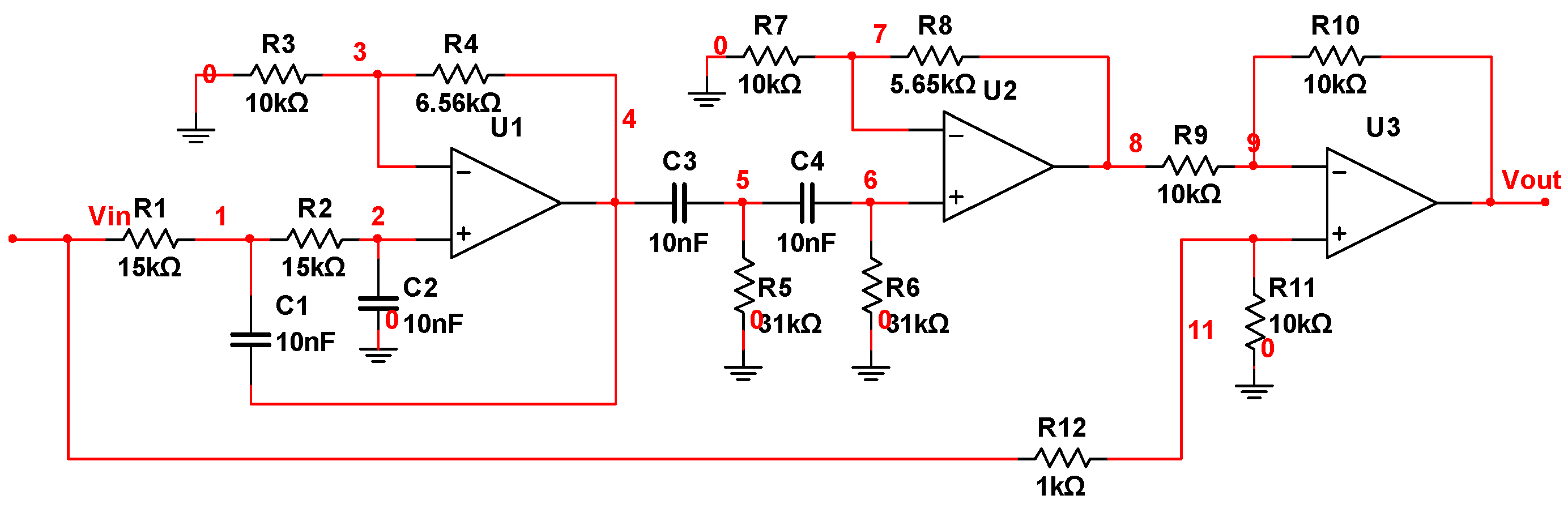
5.2. Three-Opamp Active Band-Stop Filter Circuit
6. Conclusions
Author Contributions
Funding
Conflicts of Interest
References
- Tang, S.; Li, Z.; Chen, L. Fault Detection in Analog and Mixed-Signal Circuits by Using Hilbert-Huang Transform and Coherence Analysis; Elsevier: Amsterdam, The Netherlands, 2015. [Google Scholar]
- Wang, Y.H.; Yan, Y.Z.; Signal, S. Wavelet-based feature extraction in fault diagnosis for biquad high-pass filter circuit. Math. Probl. Eng. 2016, 2016, 1–13. [Google Scholar] [CrossRef]
- Zhang, C.L.; He, Y.G.; Yuan, LF. A Novel Approach for Diagnosis of Analog Circuit Fault by Using GMKL-SVM and PSO. J. Electron. Test.-Theory Appl. 2016, 32, 531–540. [Google Scholar] [CrossRef]
- Long, Y.; Xiong, Y.J.; He, Y.G. A new switched current circuit fault diagnosis approach based on pseudorandom test and preprocess by using entropy and Haar wavelet transform. Analog Integr. Circuits Signal Process. 2017, 91, 445–461. [Google Scholar] [CrossRef]
- Li, J.M. The Application of Dual-Tree Complex Wavelet Packet Transform in Fault Diagnosis. Agro Food Ind. Hi-Tech 2017, 28, 406–410. [Google Scholar]
- Xie, X.; Li, X.; Bi, D.; Zhou, Q.; Xie, S.; Xie, Y. Analog Circuits Soft Fault Diagnosis Using Rényi’s Entropy. J. Electron. Test. 2015, 31, 217–224. [Google Scholar] [CrossRef]
- Long, T.; Jiang, S.; Luo, H.; Deng, C. Conditional entropy-based feature selection for fault detection in analog circuits. Dyna 2016, 91, 309–318. [Google Scholar] [CrossRef]
- He, W.; He, Y.; Li, B.; Zhang, C. Analog Circuit Fault Diagnosis via Joint Cross-Wavelet Singular Entropy and Parametric t-SNE. Entropy 2018, 20, 604. [Google Scholar] [CrossRef]
- Song, P.; He, Y.; Cui, W. Statistical property feature extraction based on FRFT for fault diagnosis of analog circuits. Analog Integr. Circuits Signal Process. 2016, 87, 427–436. [Google Scholar] [CrossRef]
- Zhao, D.; He, Y. A novel binary bat algorithm with chaos and Doppler effect in echoes for analog fault diagnosis. Analog Integr. Circuits Signal Process. 2016, 87, 437–450. [Google Scholar] [CrossRef]
- Prieto-Moreno, A.; Llanes-Santiago, O.; García-Moreno, E. Principal components selection for dimensionality reduction using discriminant information applied to fault diagnosis. J. Process Control 2015, 33, 14–24. [Google Scholar] [CrossRef]
- Haddad, R.Z.; Strangas, E.G. On the Accuracy of Fault Detection and Separation in Permanent Magnet Synchronous Machines Using MCSA/MVSA and LDA. IEEE Trans. Energy Convers. 2016, 31, 924–934. [Google Scholar] [CrossRef]
- Sugiyama, M. Dimensionality Reduction of Multimodal Labeled Data by Local Fisher Discriminant Analysis. J. Mach. Learn. Res. 2007, 8, 1027–1061. [Google Scholar]
- Spina, R.; Upadhyaya, S. Linear circuit fault diagnosis using neuromorphic analyzers. IEEE Trans. Circuits Syst. II Analog Digit. Signal Process. 1997, 44, 188–196. [Google Scholar] [CrossRef]
- Jia, W.; Zhao, D.; Shen, T.; Ding, S.; Zhao, Y.; Hu, C. An optimized classification algorithm by BP neural network based on PLS and HCA. Appl. Intell. 2015, 43, 1–16. [Google Scholar] [CrossRef]
- Yuan, Z.; He, Y.; Yuan, L. Diagnostics Method for Analog Circuits Based on Improved KECA and Minimum Variance ELM. IOP Conf. Ser.Mater. Sci. Eng. 2017. [Google Scholar] [CrossRef]
- Yu, W.X.; Sui, Y.; Wang, J. The Faults Diagnostic Analysis for Analog Circuit Based on FA-TM-ELM. J. Electron. Test. 2016, 32, 1–7. [Google Scholar] [CrossRef]
- Ma, Q.; He, Y.; Zhou, F. A new decision tree approach of support vector machine for analog circuit fault diagnosis. Analog Integr. Circuits Signal Process. 2016, 88, 455–463. [Google Scholar] [CrossRef]
- Cui, Y.Q.; Shi, J.Y.; Wang, Z.L. Analog circuit fault diagnosis based on Quantum Clustering based Multi-valued Quantum Fuzzification Decision Tree (QC-MQFDT). Measurement 2016, 93, 421–434. [Google Scholar] [CrossRef]
- Liu, Z.B.; Jia, Z.; Vong, C.M. Capturing High-Discriminative Fault Features for Electronics-Rich Analog System via Deep Learning. IEEE Trans. Ind. Inform. 2017, 13, 1213–1226. [Google Scholar] [CrossRef]
- Zhuang, L.; Zhou, Z.; Gao, S.; Yin, J.; Lin, Z.; Ma, Y. Label Information Guided Graph Construction for Semi-Supervised Learning. IEEE Trans. Image Process. 2017, 26, 4182–4192. [Google Scholar] [CrossRef]
- Zhou, X.; Prasad, S. Active and Semisupervised Learning with Morphological Component Analysis for Hyperspectral Image Classification. IEEE Geosci. Remote Sens. Lett. 2017, 26, 1–5. [Google Scholar] [CrossRef]
- Guoming, S.; Houjun, W.; Hong, L. Analog circuit fault diagnosis using lifting wavelet transform and SVM. J. Electron. Meas. Instrum. 2010, 24, 17–22. [Google Scholar]
- Qing, Y.; Feng, T.; Dazhi, W.; Dongsheng, W.; Anna, W. Real-time fault diagnosis approach based on lifting wavelet and recursive LSSVM. Chin. J. Sci. Instrum. 2011, 32, 596–602. [Google Scholar]
- Pan, H.; Siu, W.C.; Law, N.F. A fast and low memory image coding algorithm based on lifting wavelet transform and modified SPIHT. Signal Process. Image Commun. 2008, 23, 146–161. [Google Scholar] [CrossRef]
- Hou, X.; Yang, J.; Jiang, G.; Qian, X. Complex SAR Image Compression Based on Directional Lifting Wavelet Transform with High Clustering Capability. IEEE Trans. Geosci. Remote Sens. 2013, 51, 527–538. [Google Scholar] [CrossRef]
- Roy, A.; Misra, A.P. Audio signal encryption using chaotic Hénon map and lifting wavelet transforms. Eur. Phys. J. Plus 2017, 132, 524. [Google Scholar] [CrossRef]
- Chiang, L.H.; Kotanchek, M.E.; Kordon, A.K. Fault diagnosis based on Fisher discriminant analysis and support vector machines. Comput. Chem. Eng. 2004, 28, 1389–1401. [Google Scholar] [CrossRef]
- Yin, Y.; Hao, Y.; Bai, Y.; Yu, H. A Gaussian-based kernel Fisher discriminant analysis for electronic nose data and applications in spirit and vinegar classification. J. Food Meas. Charact. 2017, 11, 24–32. [Google Scholar] [CrossRef]
- Li, C.; Jiang, K.; Zhao, X.; Fan, P.; Wang, X.; Liu, C. Spectral identification of melon seeds variety based on k-nearest neighbor and Fisher discriminant analysis. In Proceedings of the AOPC 2017: Optical Spectroscopy and Imaging, Beijing, China, 4–6 June 2017. [Google Scholar]
- Wang, Z.; Ruan, Q.; An, G. Facial expression recognition using sparse local Fisher discriminant analysis. Neurocomputing 2016, 174, 756–766. [Google Scholar] [CrossRef]
- Yu, Q.; Wang, R.; Li, B.N.; Yang, X.; Yao, M. Robust Locality Preserving Projections With Cosine-Based Dissimilarity for Linear Dimensionality Reduction. IEEE Access 2017, 5, 2676–2684. [Google Scholar] [CrossRef]
- Sugiyama, M.; Idé, T.; Nakajima, S.; Sese, J. Semi-supervised local Fisher discriminant analysis for dimensionality reduction. Mach. Learn. 2010, 78, 35. [Google Scholar] [CrossRef]
- Wang, S.; Lu, J.; Gu, X.; Du, H.; Yang, J. Semi-supervised linear discriminant analysis for dimension reduction and classification. Pattern Recognit. 2016, 57, 179–189. [Google Scholar] [CrossRef]
- Cheng, G.; Zhu, F.; Xiang, S.; Wang, Y.; Pan, C. Semisupervised Hyperspectral Image Classification via Discriminant Analysis and Robust Regression. IEEE J. Sel. Top. Appl. Earth Obs. Remote Sens. 2017, 9, 595–608. [Google Scholar] [CrossRef]
- Blum, A.; Mitchell, T. Combining labeled and unlabeled data with co-training. In Proceedings of the Eleventh Annual Conference on Computational Learning Theory, Madison, WI, USA, 24–26 July 1998; pp. 92–100. [Google Scholar]
- Zhao, J.H.; Wei-Hua, L.I. One of semi-supervised classification algorithm named Co-S3OM based on cooperative training. Appl. Res. Comput. 2013, 30, 3237–3239. [Google Scholar]
- Díaz-Uriarte, R.; De Andres, S.A. Gene selection and classification of microarray data using random forest. BMC Bioinform. 2006, 7, 3. [Google Scholar] [CrossRef] [PubMed]
- Belgiu, M.; Drăguţ, L. Random forest in remote sensing: A review of applications and future directions. ISPRS J. Photogramm. Remote Sens. 2016, 114, 24–31. [Google Scholar] [CrossRef]
- Li, C.; Sanchez, R.V.; Zurita, G.; Cerrada, M.; Cabrera, D.; Vásquez, R.E. Gearbox fault diagnosis based on deep random forest fusion of acoustic and vibratory signals. Mech. Syst. Signal Process. 2016, 76, 283–293. [Google Scholar] [CrossRef]
- Mellor, A.; Boukir, S.; Haywood, A.; Jones, S. Exploring issues of training data imbalance and mislabelling on random forest performance for large area land cover classification using the ensemble margin. ISPRS J. Photogramm. Remote Sens. 2015, 105, 155–168. [Google Scholar] [CrossRef]
- Jiang, Y.; Wang, Y.; Luo, H. Fault diagnosis of analog circuit based on a second map SVDD. Analog Integr. Circuits Signal Process. 2015, 85, 395–404. [Google Scholar] [CrossRef]


| Fault ID | Fault Mode | Nominal | Faulty Value and Variation Percentage |
|---|---|---|---|
| F0 | normal | --- | --- |
| F1 | C1↑ | 5 nF | 5 nF (1 + 50%) 5 nF (1 + 100%) |
| F2 | C1↓ | 5 nF | 5 nF (1 − 80%) 5 nF (1 − 50%) |
| F3 | C2↑ | 5 nF | 5 nF (1 + 50%) 5 nF (1 + 100%) |
| F4 | C2↓ | 5 nF | 5 nF (1 − 80%) 5 nF (1 − 50%) |
| F5 | R2↑ | 3 kΩ | 3 kΩ (1 + 50%) 3 kΩ (1 + 100%) |
| F6 | R2↓ | 3 kΩ | 3 kΩ (1 − 80%) 3 kΩ (1 − 50%) |
| F7 | R3↑ | 2 kΩ | 2 kΩ (1 + 50%) 2 kΩ (1 + 100%) |
| F8 | R3↓ | 2 kΩ | 2 kΩ (1 − 80%) 2 kΩ (1 − 50%) |
| Fault ID | Fault Type | Nominal | Method 1 [9] | Method 2 [3] | Method 3 [17] | Proposed Method | ||||
|---|---|---|---|---|---|---|---|---|---|---|
| Fault Value | Accuracy | Fault Value | Accuracy | Fault Value | Accuracy | Fault Value | Accuracy | |||
| F0 | normal | --- | --- | 97.2% | --- | 99% | --- | 100% | --- | 100% |
| F1 | C1↑ | 5 nF | 7.5 nF | 99% | 10 nF | 100% | 7.5 nF | 95% | 7.5 nF 10 nF | 100% |
| F2 | C1↓ | 5 nF | 2.5 nF | 100% | 2.5 nF | 100% | 2.5 nF | 100% | 1 nF 2.5 nF | 100% |
| F3 | C2↑ | 5 nF | 7.5 nF | 96% | 10 nF | 100% | 7.5 nF | 90% | 7.5 nF 10 nF | 100% |
| F4 | C2↓ | 5 nF | 2.5 nF | 97% | 2.5 nF | 100% | 2.5 nF | 100% | 1 nF 2.5 nF | 100% |
| F5 | R2↑ | 3 kΩ | 4.5 kΩ | 98% | 6 kΩ | 99.3% | 4.5 kΩ | 100% | 4.5 kΩ 6 kΩ | 98% |
| F6 | R2↓ | 3 kΩ | 1.5 kΩ | 100% | 1.5 kΩ | 99.3% | 1.5 kΩ | 100% | 0.6 kΩ 1.5 kΩ | 95% |
| F7 | R3↑ | 2 kΩ | 3 kΩ | 100% | 4 kΩ | 100% | 3 kΩ | 95% | 3 kΩ 4 kΩ | 100% |
| F8 | R3↓ | 2 kΩ | 1 kΩ | 98.6% | 1 kΩ | 100% | 1 kΩ | 100% | 0.4 kΩ 1 kΩ | 100% |
| Fault ID | Fault Mode | Nominal | Faulty Value and Variation Percentage |
|---|---|---|---|
| F0 | --- | --- | --- |
| F1 | C1↑C2↑ | 5 nF 5 nF | 5 nF (1 + 50%) 5 nF (1 + 100%) 5 nF (1 + 50%) 5 nF (1 + 100%) |
| F2 | C1↓C2↓ | 5 nF 5 nF | 5 nF (1 − 80%) 5 nF (1 − 50%) 5 nF (1 − 80%) 5 nF (1 − 50%) |
| F3 | R2↑R3↑ | 3 kΩ 2 kΩ | 3 kΩ (1 + 50%) 3 kΩ (1 + 100%) 2 kΩ (1 + 50%) 2 kΩ (1 + 100%) |
| F4 | R2↓R3↓ | 3 kΩ 2 kΩ | 3 kΩ (1 − 80%) 3 kΩ (1 − 50%) 2 kΩ (1 − 80%) 2 kΩ (1 − 50%) |
| F5 | R2↑C1↑ | 3 kΩ 5 nF | 3 kΩ (1 + 50%) 3 kΩ (1 + 100%) 5 nF (1 + 50%) 5 nF (1 + 100%) |
| F6 | R2↑C2↓ | 3 kΩ 5 nF | 3 kΩ (1 + 50%) 3 kΩ (1 + 100%) 5 nF (1 − 80%) 5 nF (1 − 50%) |
| F7 | R3↓C1↑ | 2 kΩ 5 nF | 2 kΩ (1 − 80%) 2 kΩ (1 − 50%) 5 nF (1 + 50%) 5 nF (1 + 100%) |
| F8 | R3↓C2↓ | 2 kΩ 5nf | 2 kΩ (1 − 80%) 2 kΩ (1 − 50%) 5 nF (1 − 80%) 5 nF (1 − 50%) |
| Fault ID | F0 | F1 | F2 | F3 | F4 | F5 | F6 | F7 | F8 |
|---|---|---|---|---|---|---|---|---|---|
| Accuracy | 100% | 100% | 100% | 100% | 96% | 100% | 100% | 98% | 94% |
| Fault ID | Fault Mode | Nominal | Faulty Value and Variation Percentage |
|---|---|---|---|
| F0 | normal | --- | --- |
| F1 | C4open | 10 nF | 100 MΩ |
| F2 | R1↑ | 15 kΩ | 15 kΩ (1 + 20%) 15 kΩ (1 + 50%) |
| F3 | R2↑ | 15 kΩ | 15 kΩ (1 + 20%) 15 kΩ (1 + 50%) |
| F4 | C2↓ | 10 nF | 10 nF (1 − 50%) 10 nF (1 − 20%) |
| F5 | C3↑ | 10 nF | 10 nF (1 + 50%) 10 nF (1 + 100%) |
| F6 | R8↓ | 5.65 kΩ | 5.65 kΩ (1 − 80%) 5.65 kΩ (1 − 50%) |
| F7 | R9↑ | 10 kΩ | 10 kΩ (1 + 50%) 10 kΩ (1 + 100%) |
| F8 | R10↓ | 10 kΩ | 10 kΩ (1 − 80%) 10 kΩ (1 − 50%) |
| F9 | R11↑ | 10 kΩ | 10 kΩ (1 + 50%) 10 kΩ (1 + 100%) |
| F10 | R5↓ and R6↑ and C2↓ | 31 kΩ 31 kΩ 10 nF | 31 kΩ (1 − 50%) 31 kΩ (1 − 20%) 31 kΩ (1 + 20%) 31 kΩ (1 + 50%) 10 nF (1 − 50%) 10 nF (1 − 20%) |
| F11 | R8↓ and R9↑ and C3↑ | 5.65 kΩ 10 kΩ 10 nF | 5.65 kΩ (1 − 50%) 5.65 kΩ (1 − 20%) 10 kΩ (1 + 20%) 10 kΩ (1 + 50%) 10 nF (1 + 20%) 10 nF (1 + 50%) |
| F12 | R10↓ and R11↑ | 10 kΩ 10 kΩ | 10 kΩ (1 − 50%) 10 kΩ (1 − 20%) 10 kΩ (1 + 20%) 10 kΩ (1 + 50%) |
| Fault ID | Fault Type | Nominal | Method1 [42] | Proposed Method |
|---|---|---|---|---|
| Fault Value | Fault Value | |||
| F0 | normal | --- | --- | --- |
| F1 | C4open | 10 nF | C4open | 100MΩ |
| F2 | R1↑ | 15 kΩ | 15 kΩ (1 + 20%) | 15 kΩ (1 + 20%) 15 kΩ (1 + 50%) |
| F3 | R2↑ | 15 kΩ | 15 kΩ (1 + 20%) | 15 kΩ (1 + 20%) 15 kΩ (1 + 50%) |
| F4 | C2↓ | 10 nF | 10 nF (1 − 20%) | 10 nF (1 − 50%) 10 nF (1 − 20%) |
| F5 | C3↑ | 10 nF | 10 nF (1 + 50%) | 10 nF (1 + 50%) 10 nF (1 + 100%) |
| F6 | R8↓ | 5.65 kΩ | 5.65 kΩ (1-50%) | 5.65 kΩ (1 − 80%) 5.65 kΩ (1 − 50%) |
| F7 | R9↑ | 10 kΩ | 10 kΩ (1 + 50%) | 10 kΩ (1 + 50%) 10 kΩ (1 + 100%) |
| F8 | R10↓ | 10 kΩ | 10 kΩ (1-50%) | 10 kΩ (1 − 80%) 10 kΩ (1 − 50%) |
| F9 | R11↑ | 10 kΩ | 10 kΩ (1 + 50%) | 10 kΩ (1 + 50%) 10 kΩ (1 + 100%) |
| F10 | R5↓ and R6↑ and C2↓ | 31 kΩ 31 kΩ 10 nF | 31 kΩ (1 − 20%) 31 kΩ (1 + 20%) 10 nF (1 − 20%) | 31 kΩ (1 − 50%) 31 kΩ (1 − 20%) 31 kΩ (1 + 20%) 31 kΩ (1 + 50%) 10 nF (1 − 50%) 10 nF (1 − 20%) |
| F11 | R8↓ and R9↑ and C3↑ | 5.65 kΩ 10 kΩ 10 nF | 5.65 kΩ (1 − 80%) 10 kΩ (1 + 20%) 10 nF (1 + 20%) | 5.65 kΩ (1 − 50%) 5.65 kΩ (1 − 20%) 10 kΩ (1 + 20%) 10 kΩ (1 + 50%) 10 nF (1 + 20%) 10 nF (1 + 50%) |
| F12 | R10↓ and R11↑ | 10 kΩ 10 kΩ | 10 kΩ (1 − 20%) 10 kΩ (1 + 20%) | 10 kΩ (1 − 50%) 10 kΩ (1 − 20%) 10 kΩ (1 + 20%) 10 kΩ (1 + 50%) |
| Average fault diagnosis | 93.08% | 98.2% |
© 2019 by the authors. Licensee MDPI, Basel, Switzerland. This article is an open access article distributed under the terms and conditions of the Creative Commons Attribution (CC BY) license (http://creativecommons.org/licenses/by/4.0/).
Share and Cite
Wang, L.; Zhou, D.; Tian, H.; Zhang, H.; Zhang, W. Parametric Fault Diagnosis of Analog Circuits Based on a Semi-Supervised Algorithm. Symmetry 2019, 11, 228. https://doi.org/10.3390/sym11020228
Wang L, Zhou D, Tian H, Zhang H, Zhang W. Parametric Fault Diagnosis of Analog Circuits Based on a Semi-Supervised Algorithm. Symmetry. 2019; 11(2):228. https://doi.org/10.3390/sym11020228
Chicago/Turabian StyleWang, Ling, Dongfang Zhou, Hui Tian, Hao Zhang, and Wei Zhang. 2019. "Parametric Fault Diagnosis of Analog Circuits Based on a Semi-Supervised Algorithm" Symmetry 11, no. 2: 228. https://doi.org/10.3390/sym11020228
APA StyleWang, L., Zhou, D., Tian, H., Zhang, H., & Zhang, W. (2019). Parametric Fault Diagnosis of Analog Circuits Based on a Semi-Supervised Algorithm. Symmetry, 11(2), 228. https://doi.org/10.3390/sym11020228