1. Introduction
There a lot of things that can be carried out when we talk about digital imagery. Ideally, in this multimedia world, it is important to ensure that you offer the best visualization of scenes. Simple digital cameras capture objects and their environmental information in such a way that each data point (also called a pixel) is represented in two dimensions
x and
y. An image provides assorted features about a scene like the shape of an object, its color and its texture. However, the most realistic type of data is three-dimensional (3D) data which is a Point Cloud, which contains another dimension of depth along-with length and width. Technically, a point cloud is a database or set of points in space containing data in 3D (
&
z) coordinate system. We are living in, moving through and seeing the world in three dimensions and a point cloud simulates objects and their environment as we see them through our own eyes. The chief concern is that a point cloud is an accurate digital record of objects and scenes. Generally, point clouds are produced by 3D systems, like Microsoft Kinect, Light Detection and Ranging (LiDAR) that actively acquire accurate and dense point clouds of the environment and provide useful data, which consists of 3D points with geometric and color information [
1]. Microsoft Kinect hardware consists of an RGB-Camera and a depth sensor from which the prior detects red, green and blue colors of the object and then uses infrared invisible rays to measure the depth and create 3D point clouds. LiDAR systems used light waves from LASER to measure the depth of an object. It calculates how long it takes for the light to hit an object and reflect back. The distance is calculated using the velocity of light [
2]. The images provide less information than point clouds because the former represent pixels in two dimensions
x &
y and the latter utilize three dimensions
&
z for each point. This enormous information enriches point cloud usage in multiple fields such as robotics, 3D modeling of architecture, agriculture and industrial automation [
3]. The use of point clouds is increasing day by day from 3D games to real-time robotic applications and it is difficult to process such types of massive information. A point cloud requires an additional storage space penalty to represent a scene as compared to images due to additional coordinate
z. Therefore, the availability of a depth sensor in hand-held and head-mounted devices has increased the need for memory management for depth information on smart devices. This can also help to reduce the requirement of bandwidth for data transfer over the network.
In robotics real-time environment, bandwidth to transfer 3D data on network and storage space requirements demand to compress point clouds up to a maximum level and minimize memory requirements without disturbing the entire structure of objects or scenes. Various 3D compression techniques stand in the literature which can be classified as Lossy and Lossless. These are the characterizations used to explicate the distinction between two file compression formats. These terms can be elaborated on the basis of information lost. The lossless compression techniques do not involve the loss of information [
4,
5]. These are very applicable where we cannot tolerate the difference between original and reconstructed data. On the other hand, the lossy compression techniques are associated with minor loss of information. The file size is reduced in such techniques by permanently eliminating the certain information. The reconstructed data acquired from decompression phase is closely matching to the original one but not exactly. This compression results in loss of quality and reconstructed point cloud admit some errors [
6,
7]. So, the applications that utilize lossy compression techniques have to tolerate the difference between reconstructed and original data [
8,
9]. Several lossy compression techniques compress point clouds by using an efficient data structure like An octree [
10,
11]. Octree is a tree like data structure in which each internal node has exactly eight children. It divides a 3D point cloud by recursively subdividing it into eight octants. A fast variant of Gaussian Mixture Model and an Expectation-Maximization algorithm is used in [
12] that replaces points with a set of Gaussian distribution. Delaunay triangulation for a given set of points
P in a plane is a triangulation such that no point is inside the circumcircle of any triangle.
We propose a novel lossy point cloud compression and decompression technique in which a point cloud is first partitioned into a set of segments and planes are extracted from each segment. Then, each plane is represented by a polynomial equation of degree one that is also called a planer equation. This technique is very capable of reconstructing a surface by using polynomial equation coefficients and boundary conditions of a particular surface that is normally an
-concave hull. The proposed algorithm is evaluated based on three parameters compression ratio, Root-Mean-Square Error (RMSE) and time required for compression and decompression process on publicly available 3D point cloud datasets. The rest of the paper is organized as follows: Existing techniques are discussed in
Section 2, methodology is expressed in
Section 3, results are discussed in
Section 4 and
Section 5.
Section 6 concludes the work.
2. Related Work
Several point cloud compression approaches exist in the literature that optimize the storage space and bandwidth requirements. The lossy compression techniques [
6,
13,
14,
15] optimize storage requirements up to a significant level but reconstructed point cloud has structure, texture and color errors. Lossless compression is expressed in [
10] that utilizes double buffering Octree data structure to detect spatial and temporal changes in the stream of point clouds with the objective of optimizing memory requirements and processing latency to process real-time point cloud. The compression performance is measured based on two parameters, bits required to present each point and loss of quality is measured as the symmetric root-mean-square distance between the non-quantized and decompressed point cloud. The compression rate is increased in [
10] by 10% as compared to state-of-the-art techniques. Another efficient implementation of Octree data structure is exercised in [
11] to compress 3D point clouds data without any loss of information. An octree is the generalized form of binary trees and quad-trees, that store one and two-dimensional data respectively. Generally, each node in an octree represents the volume formed by a rectangular cuboid, but [
11] enhanced that strategy and simplified to an axis aligned cube. In addition, they are focused on individual points compression, far from determining the geometry of surfaces. Normally, a Terrestrial laser scanner takes four bytes of memory to store each point in three dimensions and [
11] used Octree in an efficient way and optimized memory requirement for each point up to two bytes. So, the whole point cloud is compressed up to
, which is a numerable contribution in lossless compression techniques.
A 3D mesh is the structural build of a 3D model consisting of polygons. 3D meshes use reference points in X, Y and Z axes to define shapes with height, width and depth. Polygons are a collection of vertices, edges and faces that define the shape of a polyhedral object. The faces usually consist of squares, rectangles (triangle mesh), quadrilateral or convex polygons. This small 3D meshes compression leads to point cloud memory optimization. A survey on mesh compression techniques is presented in [
16] and another evaluation framework for 3D mesh compression is expressed in [
17] in which authors claimed to have achieved a compression ratio 10 to 60%. A lossy compression model based on Hierarchical point clustering is exercised in [
18] that focused on geometry of points. It generated Coarser Level of Detail (LOD) during point clustering phase. LOD hierarchy is further traversed in top-down order to update the geometry of each associated child. A real-time point cloud compression is described in [
13] that decomposes the data chunks into voxels and then these are compressed individually. It supports both static and real-time point cloud compression in an online application. Voxel grid size can be controlled implicitly but compression ratio decreased with voxel size and it is difficult to choose the trade-off between compression ratio and locality.
Miguel Cazorla [
12] contributions in the field of 3D point cloud lossy compression are prodigious. First, he proposed a data set composed of a set of 3D point clouds and also provided tools for comparing and evaluating compression methods based on compression level and distance parameters in [
8]. These data sets are well organized and mainly categorized into two classes, real and synthetic types. Each category is further classified into three classes with respect to the structure of objects and texture available in the scene. Three classes are the high, medium and low structure in which high structured means more surfaces are planer and low means complex data structure. Furthermore, high texture means more text available in the scene and vice versa. The above discussed data sets [
8] are published in a well-known journal and these are publicly available under the license and further utilized in Miguel Cazorla compression methods [
7,
12]. They mainly concentrated on geometric characteristics of objects and scenes to compress point clouds. First, it utilized the advantageous aspects of Delaunay triangles to compress 3D surfaces in [
7]. The point cloud is first segmented into a set of planes and then points under each plane are computed. Further, these points are represented with Delaunay triangles that lead to compression of surfaces. That framework was tested on [
8] datasets and performance was evaluated based on two parameters, Compression ratio and Root-Mean-Square-Error (RMSE) between original and reconstructed point cloud. Furthermore, it achieved 55%–85% compression ratio with 0.5 RMSE. The compression technique proposed in [
7] is further extended in [
12] by the same author in which it utilized Gaussian Mixture Models (GMMs) and an Expectation-Maximization algorithm to compress point cloud data. The points of interest are selected as a first step in [
12]. These points are the best candidates to perform compression which are addressed by the planer patch extraction method as defined in [
7]. Here GMMs are used to compress these points that hold the data as 3D multivariate Gaussian distribution, which allows the reconstruction of the original data with a certain statistical reliability. The performance of [
12] is evaluated by using [
8] datasets and the compression ratio is achieved up to 85.25% with RMSE of
.
We propose a novel lossy 3D point cloud compression method in which a point cloud is compressed in such a way that a set of points is represented by Polynomial equation of degree one that utilizes geometric information of scenes as highlighted by many researchers [
19,
20,
21,
22,
23]. We used the framework illustrated in [
24] for selection of points of interest which are the best candidates to represent a planer surface. Further, each plane is stored in the form of a polynomial equation of degree one coefficient instead of preserving points itself. We also preserve the boundary condition of each plane which helps us in the decompression phase. The proposed algorithm is tested on datasets described in [
8] and these are utilized in previous techniques as a standard. Performance is evaluated based on three parameters, compression ratio, RMSE and compression and decompression time. The results are also compared with state-of-the-art lossy and lossless point cloud compression techniques. We achieved 89% compression ratio on average on highly structured data sets with lesser RMSE of
.
3. Methodology
A raw point cloud may contain noise due to sensor limitations that result in unstable feature estimations. Therefore, reduction of noise becomes necessary, while it preserves features with its fine detail. A prior step to process a point cloud is to discard noisy points. These are normally referred to as Outliers. Therefore, noise removal techniques such as Voxel Grid filter, (Radius, Conditional & Statistical) Outlier Removal filters [
25,
26,
27] are employed to reduce the effects of noise from a 3D point cloud. We use statistical outlier removal filter due to its lesser computational time and better results as compared to state-of-the-art filters [
28]. In this filter, unwanted points are highlighted and discarded based on neighborhood information of each point. Mean distance and standard deviation of each point are computed to highlight noise and is tested for its being noisy or not. After detecting outliers, these points are trimmed out and filtered point cloud is provided for further processing.
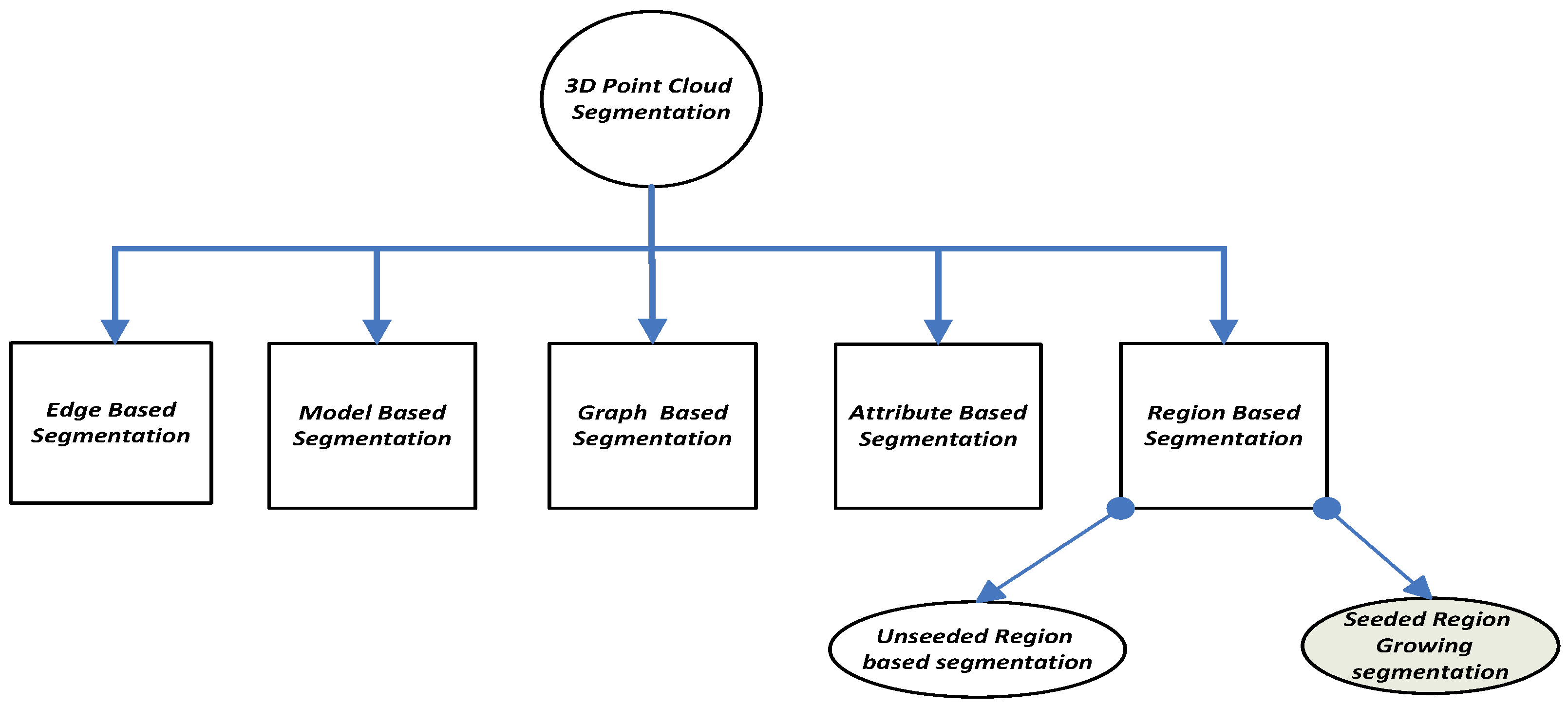
3.1. Seeded Region Growing Segmentation
Segmentation is a process in which we divide a set of points into multiple segments. Here, the purpose of segmentation is to simplify the entire structure of a point cloud and to make it easier for further processing. In this process, a label is assigned to each point in such a way that every point of cloud belongs to any of its segments and this apportionment is done based on common attributes of points. As a result, a set of segments is received that covers all the points collectively. All the points in the same segment share abundant attributes like point normal, curvature value, angular distance, etc. Generally, segmentation is categorized into five classes: Edge-based, Model-based, Graph-based, Attribute-based and Region-based segmentation [
29], as shown in the
Figure 1.
The fundamental edge detection techniques are discussed in [
30] and considerable advancements are obtained but the issues of sensitivity to noise and uneven density of point clouds may cause errors or inaccurate segmentation. Model-Based Segmentation techniques are efficient but the probability of inaccuracy arises when dealing with different point cloud sources [
31].
Region growing based segmentation techniques use neighborhood information to merge those points in a region that hold similar properties and also isolate them from dissimilar properties regions. Region growing segmentation is further classified into two classes: unseeded and seeded region growing segmentation. The former is a top-down approach that considers the whole point cloud as a single region and makes segments by traversing it like a tree from top to bottom. The latter is a seeded region growing segmentation which is a bottom-up approach that selects a point as a seed and makes clusters of related points. This process iterates multiple times until all the points are to be the part of any segment. Two conceptions are involved in region growing process, intra and inter-segment distance. The angular distance between points of the same segment is known as intra-segment distance and the distance between centroids of two different segments is known as inter-segment distance. In this research, the concept of lower intra-and higher inter-segment distance is populated to make surfaces more robust, as it is an indication of fruitful segmentation. The reason to use region growing segmentation in this research is that it partitions a point cloud based on the geometry of points and our proposed novel method is closely related to it, which also concentrates on the geometry of surfaces to present them in the form of polynomial equations.
Here we demonstrate an overview of the seeded region growing process. The first step is the selection of a seed point which is considered as a base to form clusters. The region grows up on the selected seed point by testing and adding other neighborhood similar properties points that meet the defined criteria as shown in
Figure 2. When the first region is matured considerably, another seed point is selected from the rest of the cloud and a new region is formed. This cluster formation process is repeated until all the points are included in any of this cloud segment. In the beginnings, the seed selection process was a manual activity, but nowadays it is automated, based on the curvature information of points. The geometric properties of point cloud i.e., curvature information and the normal vector of points is estimated with the help of Principal Component Analysis (PCA). The imperative step in curvature estimation is the computation of covariance matrix
C which is estimated by Equation (
1).
in Equation (
1) can be calculated by Equation (
2).
is the centroid (Arithmetic Mean) of the neighborhood points
of point
P. Neighborhood points
of each point
P are highlighted by k-d tree search algorithm. K-d tree algorithm is applied here due to several reasons illustrated below. It takes
(log n) computation time that is the least time as compared to other search algorithms i.e., KNN that takes
(nd) time. K-d tree data structure having the ability to represent points in
k dimensions and it is broad into exercise to represent points in three-dimensional spaces for nearest neighbors search. Furthermore, at each level, all child nodes are split up against specific dimension and perpendicular hyperplane to the corresponding axis used. By this covariance matrix expressed in Equation (
1), it is possible to compute eigenvector
V (
,
and
) and its corresponding eigenvalue
(
,
and
). Eigenvalues description is given below in Equation (
3).
In Equation (
3),
A is a 3 × 3 covariance matrix,
v is a nonzero vector and
is any scalar value.
Here
approximates the point normal for point P and the curvature is estimated by Equation (
5)
A crucial parameter is the smoothness threshold that is the key element of the segmentation process. When the smoothness level is increased, spheres and other structures are considered as the part of planes and vice versa.
In the first stage, all points and their associated curvature values are added to a list, which is sorted by ascending order of . The point of minimum curvature value which therefore lies in the flattest region, is identified as the initial seed point, and is extracted from the point list.
The algorithm proceeds by finding a neighborhood support region for the seed, as follows:
k nearest neighbors of the seed point are identified from the point list.
Normal vectors of seed point and neighborhoods are compared. If a solid angle is found between the seed and neighbor point normal and the angle is less than a threshold value, then move to the next step.
Surface curvature of the seed and neighbor point are compared and the difference is noted. If the difference is less than a threshold value, then the neighbor point is removed from the point list and added to current seed region. This ensures that the curvature is consistent and relatively smooth within a region.
Repeat point for all neighborhood points.
The above process iterates by extracting the next seed point with minimum value from the point list, and repeating steps 1 to 3 until the point list is empty. Finally, output of the algorithm is a set of regions.
3.2. Polynomial Equations of Degree One
Here, we unfold the novelty of our proposed technique and discuss in detail how the polynomial equations of degree one are used to compress a point cloud. The output of the segmentation process discussed in
Section 3.1 is a set of regions and all points within each region are geometrically and closely related to each other. In the next step we extract planes from each region. A plane is a flat surface that extends infinitely far and it can be founded by a point and a vector perpendicular to the point. Various techniques are available to extract planes from a set of points. In this research, we have utilized Sample Consensus (SAC) method [
1] which is a standard technique for plane extraction stand in Point Cloud Library (PCL). Here we illustrate the polynomial equation and its coefficients.
Suppose
is a known point on a plane having (
) coordinates and
is a normal vector of the plane.
P is another point on a surface having coordinates (
). A vector connecting from
P to
is described in Equation (
6).
Vector (
) and
are perpendicular to each other and the dot product of two perpendicular vectors is always zero as shown in the Equation (
7).
Put the value of Equation (
6) in (
7) and calculate dot product:
After solving Equation (
8) we found:
The resultant equation of the above discussed scenario Equation (
9) is a polynomial equation of degree one that represents a planer surface. It is also called a planer equation in which
&
z are the coordinates of points belonging to that planer surface and
&
d are coefficients of equations. These coefficients are helpful to test any 3D point, either it belongs to this plane or not. A planer surface may have 100,000 points that can be represented with only four coordinates
&
d of Equation (
9) and this is the novelty of our technique. This novel approach increases compression rate dramatically and a Megabyte 3D point cloud can be stored with only a few bytes.
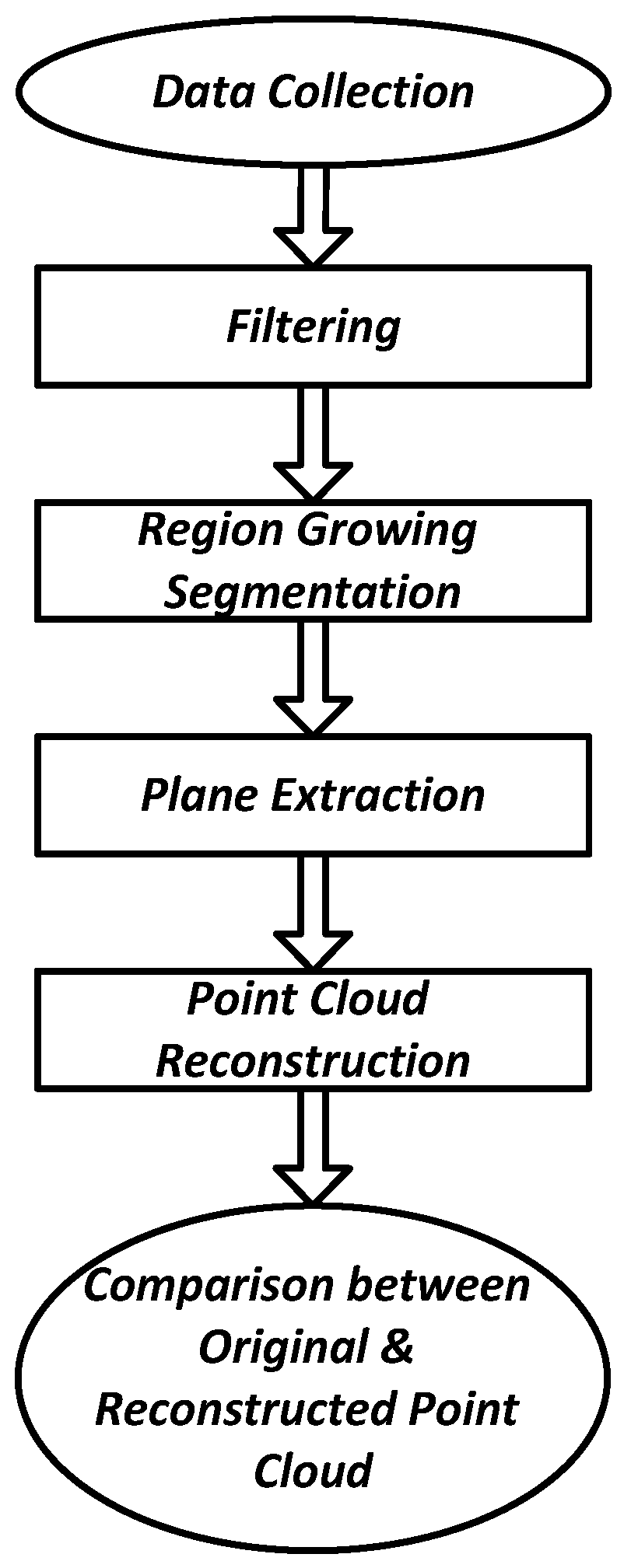
3.3. Compression
Our proposed technique is shown in the Algorithm 1 and
Figure 3 that compresses a point cloud by converting it into a data structure which is composed of plane coefficients and boundary conditions of each planer surface. This data structure is significantly smaller than the original point cloud because each segment that may contain thousands of 3D points is represented by four plane coefficients and an
-concave hull of that surface. Boundary conditions are really helpful in the decompression phase to reconstruct the point cloud.
-Concave hull is generalization of convex hull [
32], where
parameter regulates the smoothness level of the constructed hull on a data set. Furthermore, it is a concave hull with angular constrained under the minimum area condition. The illustration of the concave hull is depicted in
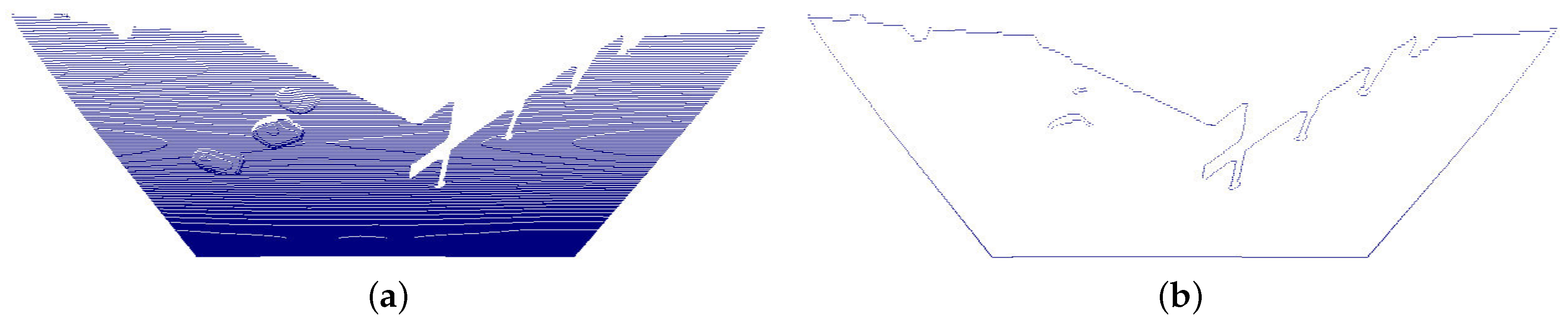
Figure 4 in which the
Figure 4a is a simple point cloud surface that requires 3250 KB of memory to store and the
Figure 4b is an
-concave hull of that surface which requires only 62 KB of memory to store. In the second stage, we indicate and discard the smallest
coordinates that further decreases the compressed file size. Finally, compressed data structure preserves only four coordinates and two-dimensional boundary of each surface. This technique optimizes the memory requirements to store and bandwidth requirements to transfer a point cloud on the network.
| Algorithm 1 Point Cloud Compression |
Require: Point Cloud: {}
Ensure: Final Planer file: {} is empty.
- 1:
Filter by applying statistical outlier removal. - 2:
Compute Point Normals {N} - 3:
Apply Region Growing Segmentation that generate List of Regions {R} - 4:
for each Region r in R do - 5:
Apply SAC method and Extract Planes {P} - 6:
for each Plane p in P do - 7:
Compute Plane Coefficients. - 8:
Estimate boundary/Concave-hull of surface. - 9:
Discard minimum coordinate. - 10:
Preserve boundary and coefficients. - 11:
end for - 12:
end for
|
3.4. Decompression
Decompression is the process of reconstructing a point cloud from the compressed file. In our proposed technique, decompression is a simple two-step process that uses a compressed data structure as input. The first step is to generate random points under the boundary conditions that were extracted in the compression phase as shown in Algorithm 2. We also care about the number of points generated under each surface and these are equal in numbers to the original surface points. These generated points have two coordinates,
x and
y. The third coordinate that shows the depth of each point is set to zero and polynomial equation of degree one (
9) is used to compute the actual value of
z coordinate. These reconstructed surfaces are merged to build a complete point cloud. After decompression, we compare original and reconstructed point cloud and measure the performance based on two parameters: compression ratio and RMSE. Compression ratio depicts how much point cloud is compressed, which is calculated by the Equation (
10).
RMS Error is an important parameter to measure the performance of the proposed algorithm illustrated below. We compute RMS error on average from original to reconstructed point cloud and vice versa. The Squared Euclidean distance is computed from a point in the first cloud to the nearest neighbor point in the second cloud and this process is repeated for all points.
| Algorithm 2 Point Cloud Decompression |
Require: ∀ Planer files list: {}
Require: Filtered Point Cloud {}
Ensure: Reconstructed Point Cloud: {} is empty
- 1:
for each Plane p in do - 2:
Generate {} under Concave-hull. - 3:
for each in do - 4:
Compute missing coordinate by Polynomial Equation of degree one. - 5:
end for - 6:
Write to . - 7:
end for
|
4. Results
Our proposed technique is tested on 3D point cloud datasets which are described in [
8] and also used in state-of-the-art techniques [
7,
12] to measure their algorithms’ performance. These are freely available under the license. These are well organized and categorical. Such properties make it favorable to evaluate our proposed algorithm and a fair comparison with other techniques. These data sets are tested in windows environment using Microsoft Visual studio 2010 framework on
Gigahertz quad core processor with 8 Gigabytes RAM. We write our code in C++ language and utilized Point Cloud Library (PCL) to process 3D point clouds. The Point Cloud Library is a large scale, open project [
1] for 2D/3D image and point cloud processing. The PCL framework contains numerous state-of-the art algorithms including filtering, feature estimation, surface reconstruction, registration, model fitting and segmentation. It provides open access to utilize existing algorithms, and to modify and build our own algorithms to process point clouds.
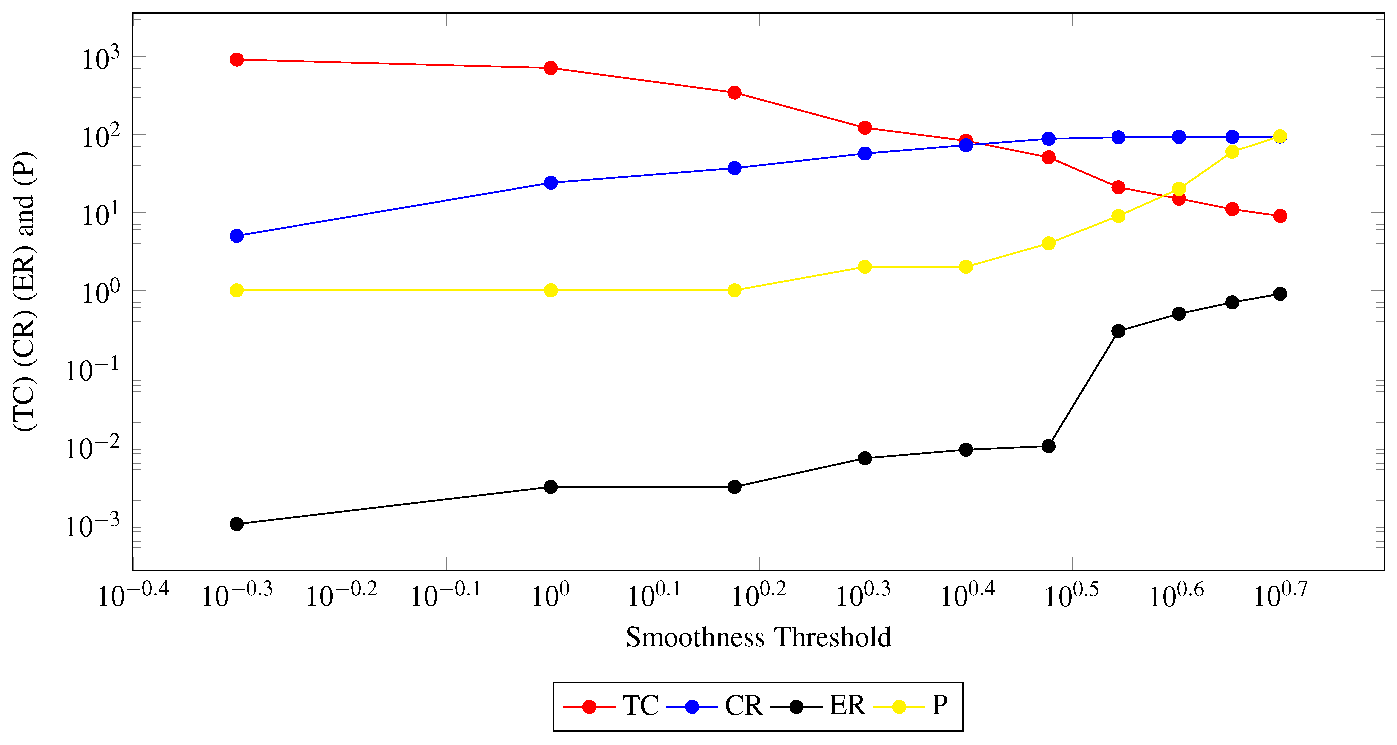
Before directly jumping into results collection, we pay special attention to parameter tuning, because parameters are the core key to computing accurate results. Here, we discuss the most vital parameter smoothness threshold and its effects on the performance of the proposed algorithm. It controls the segmentation process and clusters formation, because points inclusion in a segment is heavily dependent on a sold angle between seed and neighborhood point normal that is discussed in detail in
Section 3.1. We start from a small threshold value and gradually increase it and summarize the effects of multiple data sets on average in the
Figure 5. When the smoothness threshold is too much small, it makes 100 clusters represented as Total Clusters (TC) with a red color line in the
Figure 5. The smoothness threshold is an entry point which allows a point to be part of a segment, if the neighborhood point normal deviation from seed point is less than the threshold value then the point is included in the current segment, otherwise it makes another segment of related points. A tight threshold causes a lower number of points per segment and makes a lot of segments but the planes per segment are very low near one because plane extraction also depends on the geometry of points. Numerous segments lead to a lower compression ratio but the error rate between original and reconstructed surface is very low as shown in the
Figure 5. When the smoothness threshold increases, it increases the size of the segment and allows many points to be part of a segment, which leads to a lower number of total segments. The compression ratio is increased and the error rate is also increased; it is difficult to find a trade off between compression ratio and error rate. So, the smoothness threshold is flexible and varies according to the application’s requirements; for analysis purposes, we set it to 3 Degree at which a reasonable compression ratio is achieved within an acceptable error rate.
We test our proposed technique on different classes of data sets which are classified with respect to structural complexity and compare our results with state-of-the-art lossy and lossless techniques discussed in literature review
Section 2. A very high structure point cloud compression and decompression process is depicted in
Figure 6 and
Figure 7, results are shown in the
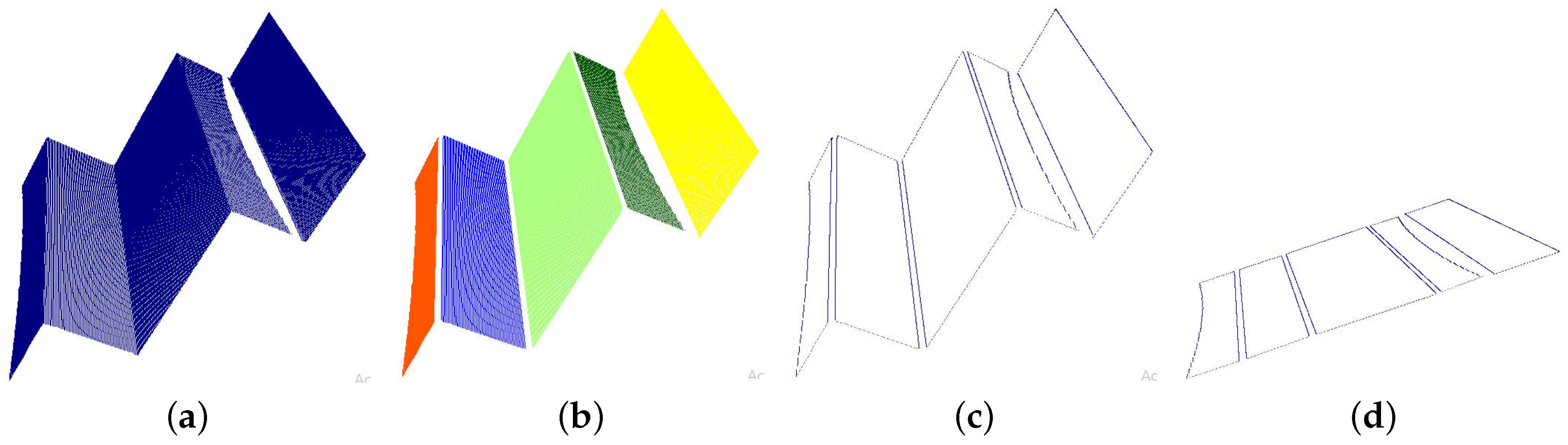
Table 1 and the illustration is given below. A Stair steps point cloud is shown in
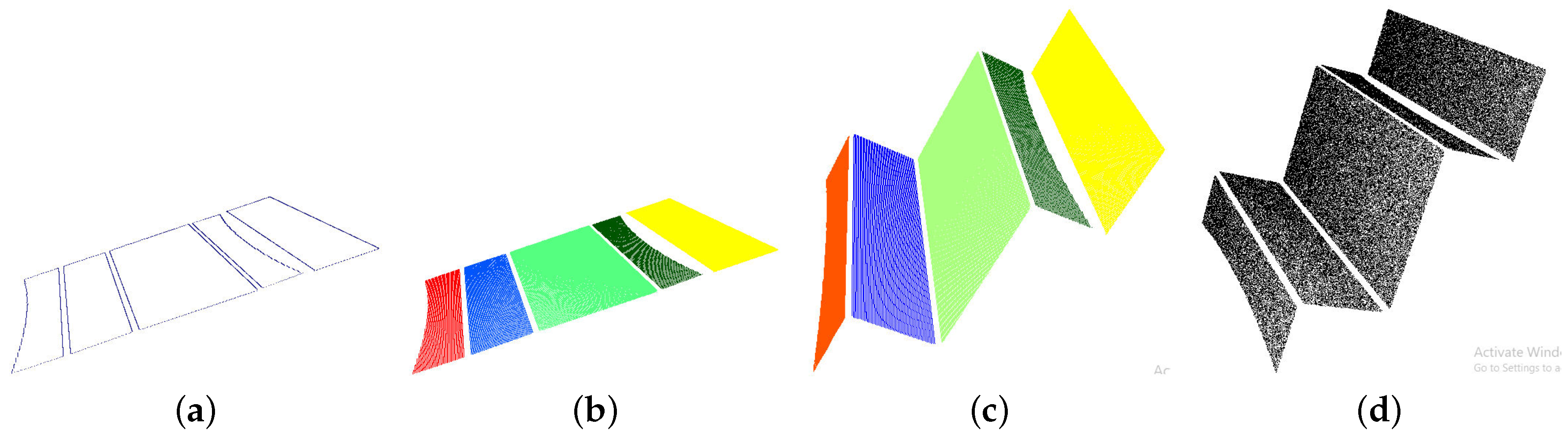
Figure 6a that has following properties: 148,039 three-dimensional points and 2719.29 KB memory to store on disk in binary format. Unnecessary points are trimmed out and set of segments is presented with different colors in the
Figure 6b that have 147,309 three-dimensional points and take 2680 KB of memory. A three-dimensional
-concave hull of segments is computed and presented in the
Figure 6c that has only 4210 three-dimensional points and takes 170 KB of memory. We have further compressed it by discarding the minimum variance coordinate of each segment and preserving two-dimensional boundary conditions of each segment in a simple text file which contains 4210 two-dimensional points and takes
KB memory. The planer coefficients are also in our accountability and prepared in a separate file, that preserves four coefficients
and
d and the total number of points under each plane for all planer surfaces that take only 2 KB of memory. A resultant compressed file that comprises the two-dimensional boundary of each segment and surface coefficients requires only 132.98 KB of memory and compression ratio is computed by Equation (
10). We compress the above discussed point cloud and optimize memory requirements up to
% which is a major contribution to our proposed techniques in the field of lossy point cloud compression. The compressed data file can be traveled on the network and requires only 5% bandwidth as compared to the original. The promising capability of our proposed technique is that it can be decompressed anywhere, independent of the compression process. The decompression phase is depicted in the
Figure 7 and the reconstructed point cloud resembles the original. The root-mean-square error between original and reconstructed point cloud is
, as shown in the
Table 1.
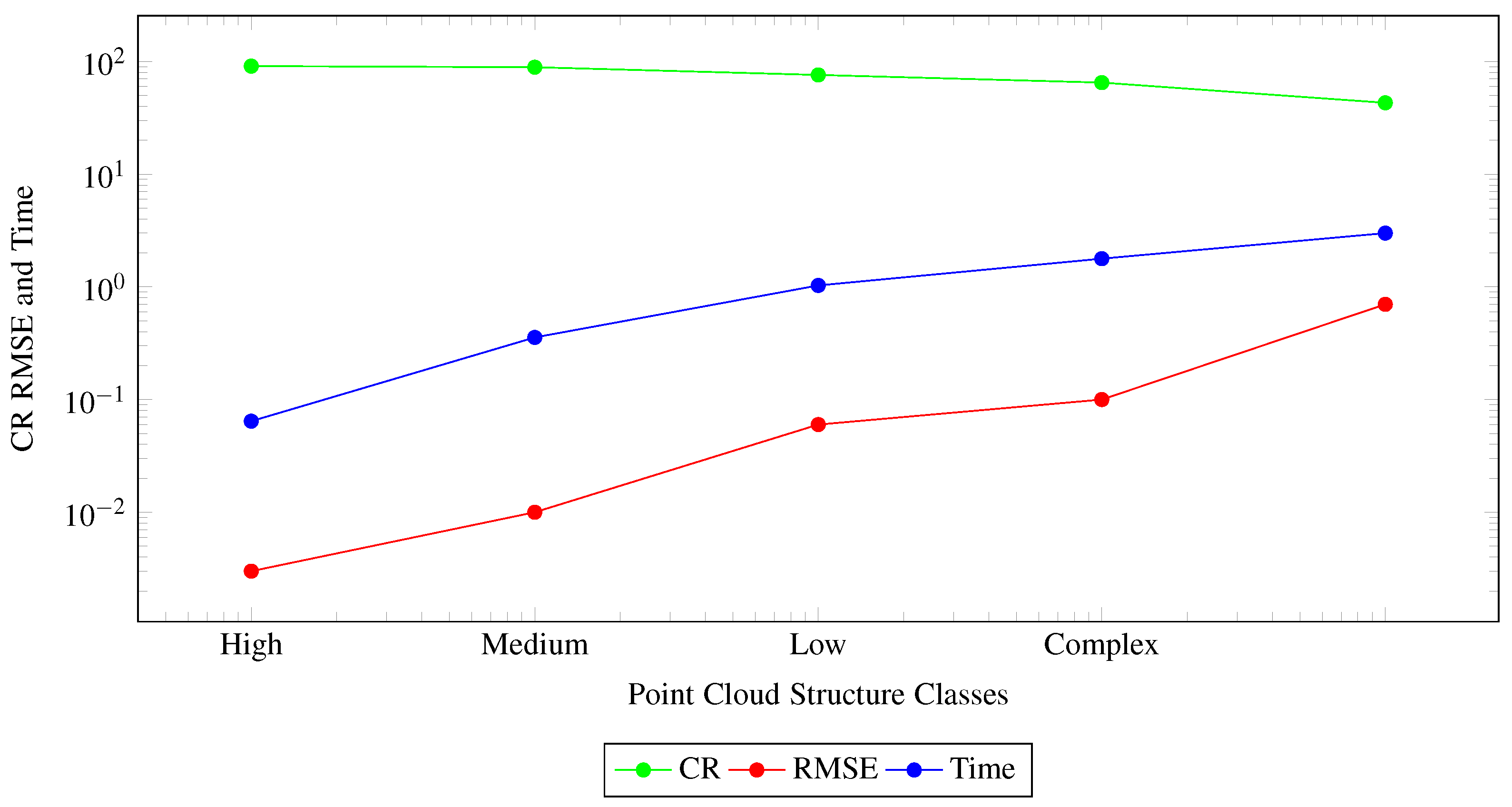
Our proposed technique is tested on four classes of datasets which can be named as high, medium, low and complex structured point clouds. We test hundreds of datasets of each class and measure compression ratio, RMSE and processing time on average of each class. It is difficult to present all the properties of each point cloud. However, we present all properties of five point clouds of each class in
Table 2. The efficiency of the algorithm on high structured point clouds is optimal in all three parameters i.e., compression ratio
achieved, RMSE
and processing time
milli seconds as shown in the
Figure 8 and
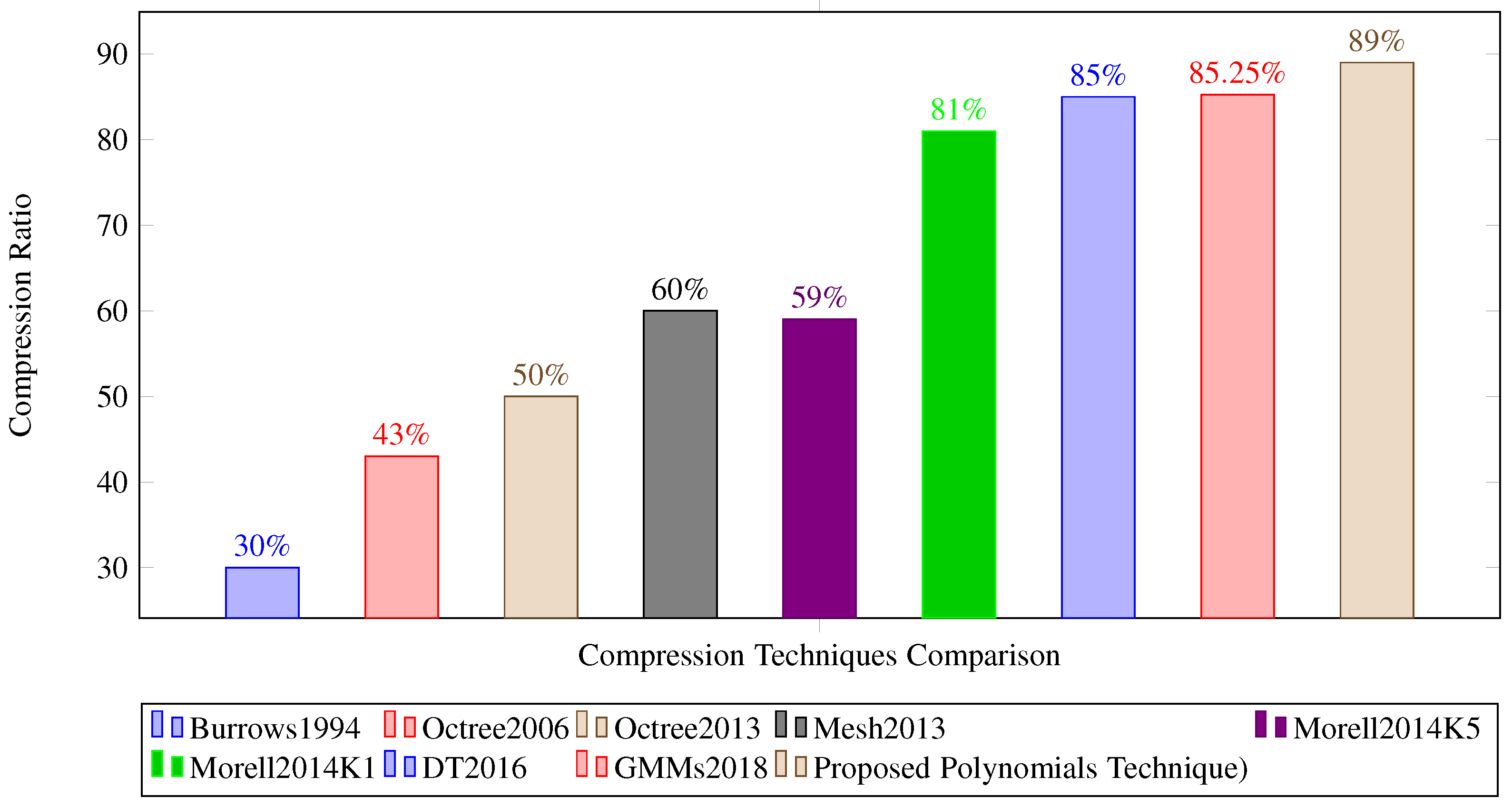
Table 2. We also compare our results with state-of-the-art compression techniques as shown in
Figure 9 and
Table 3. Several techniques are available to compress point clouds as discussed in the literature and some well-known methods are presented in
Figure 9 listed below, Burrows 1994 [
4], Octree-based point cloud compression 2006 [
10], One billion points compression based on octree data structure 2013 [
11], Morell 2014 with k = 5 and 1 [
8], Miguel Cazorle 2016 that utilized Delaunay Triangles (DT2016) [
7] and Miguel Cazorle 2018 that utilized Gaussian Mixture Model (GMMs2018) [
12]. In the late 1990s, Burrows developed a lossless compression method [
4] that can compress point cloud up to 30%. Many improvements are done in compression algorithms with the passage of time. Efficient data structures i.e., Octree, Delaunay Triangles and Gaussian Mixture Model are utilized and compress point clouds up to 85.25% with 0.1 RMSE [
12]. Our proposed technique increases compression ratio by
% on highly structured point clouds and compress up to
% with
RMSE and
ms processing time per point. This increased compression ratio leads to memory optimization and bandwidth requirements to transfer point cloud data sets on the network.
6. Conclusions
We proposed a lossy 3D point cloud compression and decompression technique. The proposed method compresses point clouds by representing implicit surfaces with polynomial equations of degree one. The compression phase consists of the segmentation process in which a point cloud is partitioned into smaller clusters based on geometric information of points. Furthermore, planes are extracted and boundary conditions are stored in a compressed file for each segment. The decompression phase reconstructs surfaces by generating two-dimensional points under boundary conditions and computes the missing third coordinate with planer equation. Our proposed algorithm is tested on multiple classes of datasets i.e., high, medium, low structured and very complex datasets and performance is evaluated based on compression ratio and root-mean-square error. We have compared the results with state-of-the-art lossless and lossy compression techniques.
Our proposed algorithm performs well on highly structured datasets and achieves compression ratio up to a significant level of 89% with 0.003 RMSE within the acceptable time scale of 0.0643 milliseconds processing time per point on average. However, the proposed method fails to deal with complex point clouds. So, it is recommended to use the proposed algorithm for highly structured datasets. The proposed technique does not deal with objects of color information. In the future, we will enhance the proposed technique to higher degree polynomials to cater to non-planer surfaces; dealing with color information is also a part of our future work.

 ,
, 


