An Analytical Numerical Method for Solving Fuzzy Fractional Volterra Integro-Differential Equations

Abstract

The modeling of fuzzy fractional integro-differential equations is a very significant matter in engineering and applied sciences. This paper presents a novel treatment algorithm based on utilizing the fractional residual power series (FRPS) method to study and interpret the approximated solutions for a class of fuzzy fractional Volterra integro-differential equations of order $0<\beta \le 1$ which are subject to appropriate symmetric triangular fuzzy conditions under strongly generalized differentiability. The proposed algorithm relies upon the residual error concept and on the formula of generalized Taylor. The FRPS algorithm provides approximated solutions in parametric form with rapidly convergent fractional power series without linearization, limitation on the problem’s nature, and sort of classification or perturbation. The fuzzy fractional derivatives are described via the Caputo fuzzy $\mathrm{H}$-differentiable. The ability, effectiveness, and simplicity of the proposed technique are demonstrated by testing two applications. Graphical and numerical results reveal the symmetry between the lower and upper $r$-cut representations of the fuzzy solution and satisfy the convex symmetric triangular fuzzy number. Notably, the symmetric fuzzy solutions on a focus of their core and support refer to a sense of proportion, harmony, and balance. The obtained results reveal that the FRPS scheme is simple, straightforward, accurate and convenient to solve different forms of fuzzy fractional differential equations.

1. Introduction

Fuzzy theory of fractional differential and integro-differential equations is a new and important branch of fuzzy mathematics. It has ample applications due to the fact that many practical problems in industrial engineering, computer science, physics, artificial intelligence, and operations research may be converted to uncertain process problems of fractional order. The topic of fuzzy fractional integro-differential equations (FFIDEs) has gained the attention of researchers in recent times because it is considered a powerful tool by which to present vague parameters and to handle with their dynamical systems in natural fuzzy environments. Indeed, it has a great significance in the fuzzy analysis theory and its applications in fuzzy control models, artificial intelligence, quantum optics, measure theory, and atmosphere, etc. [1,2,3,4]. In several cases, information about the real-life problems included is always pervaded with uncertainty. This uncertainty results from several factors, such as measurement errors, deficient data or if the constraint conditions are determined. So, it is necessary to have some mathematical tools to understand this uncertainty. Consequently, to form a convenient and applicable algorithm is important to achieve a mathematical structure that would suitably process FFIDEs and solve them.

Most FFIDE problems cannot be solved analytically, and hence, finding good approximate solutions using numerical methods will be very valuable. Recently, numerous scholars have devoted their interest to studying and investigating solutions to FFIDEs utilizing different numerical and analytical techniques; these solutions include the Fuzzy Laplace transforms technique [5], two-dimensional Legendre wavelet technique [6], Adomian decomposition technique [7], variational iteration technique [8], and the fitted reproducing kernel Hilbert space technique [9]. Besides that, other scholars have shown an interest in the existence and uniqueness of the solutions for FDEs. (For more details, see [10,11,12,13,14].) Applications of the RPS scheme are extensive and numerous, especially for the simulation of models of integer order. Such approaches have recently been developed as a powerful numerical tool for treating different problems of arbitrary order. From a methodological point of view, the Volterra integro-differential equations considered in this study under uncertainty concerned with fractional derivatives are simply generalizations of classical forms, provided that $\beta =1,$ which have various uses in physics and engineering, including in dynamical systems, nonlinear propagation of a traveling wave, damped nonlinear string, electronics, and telecommunications, etc. For more details about the integro-differential equations, refer to [15,16,17,18].

The present work aims to expand the applications of the fractional residual power series (FRPS) technique to determine approximated solutions for a class of fuzzy fractional Volterra integro-differential equations (FFVIDEs) subject to certain fuzzy initial conditions in the following form:

$$D_{a^{+}}^{\beta }y\left(x\right)+{\int }_a^x\phi \left(x,t\right)y\left(t\right)dt=g\left(x\right), x\ge a, 0<\beta \le 1,$$

(1)

with the fuzzy initial conditions

$$y\left(a\right)=y_0$$

(2)

where $\lambda$ is a parameter, $g:\left[a,b\right]\to {ℝ}_{\mathcal{F}}$ is a continuous fuzzy-valued function,$\phi \left(x,t\right)$ is a continuous crisp arbitrary kernel function, $D_{a^{+}}^{\beta }$ is the fuzzy fractional derivative in Caputo sense, $y_0\in {ℝ}_{\mathcal{F}}$ and $y\left(x\right)$ is unknown analytical fuzzy function to be determined. Throughout this paper, ${ℝ}_{\mathcal{F}}$ stands for the set of all fuzzy numbers on the real line $ℝ$.

The FRPS technique developed in [19] is considered an easy and applicable tool to create a power series solution for strongly linear and nonlinear equations without being linearized, discretized, or exposed to perturbation [20,21,22,23,24,25,26,27]. This technique is featured by the following characteristics: firstly, the method provides the solutions in Taylor expansions; therefore, the exact solutions will be available when the solutions are polynomials. Secondly, the solutions along with their derivatives can be applied for each arbitrary point in the given interval. Thirdly, the method does not require modifications while converting from the lower to the higher order. Consequently, this method can be easily and directly applied to the given system by selecting an appropriate value for the initial guesses/approximations. Fourthly, the FRPS technique needs minor computational requirements with less time and more accuracy.

The remainder of the current paper is structured as follows: In the next section, some essential notations, definitions, and results relating to fuzzy calculus and fuzzy fractional calculus are shown. The process to solve fuzzy FVIDEs is discussed in Section 3. In Section 4, the construction of solutions using the FRPS algorithm is presented. Numerical examples will be performed to show the capability, potentiality and simplicity of the method. The last section of the current paper is a conclusion.

2. Overview of Fuzzy Calculus and Fuzzy Fractional Calculus

In the current section, the essential notations, definitions and the basic results relating to fuzzy calculus and fuzzy fractional calculus are presented. In general, a fuzzy number $\rho$ is a fuzzy subset of $ℝ$ with normal, convex, and upper semi-continuous membership function of bounded support. For more details, refer to [13,28,29,30,31,32,33,34].

Definition 1.

[28]A fuzzy number$\rho$is a mapping such that$\rho :ℝ\to \left[0,1\right]$with the following properties:

• $\rho$is fuzzy convex, that is,$\rho \left(\lambda s+\left(1-\lambda \right)t\right)\ge min\left\{\rho \left(s\right),\rho \left(t\right)\right\}$for all$s,t\in ℝ$,$\lambda \in \left[0,1\right].$
• $\rho$is normal, that is,$\exists s_{*}\in ℝ$for which$\rho \left(s_{*}\right)=1$.
• $\rho$is upper-semi continuous, that is,$\rho \left(s_{*}\right)\ge li{m}_{s\to s_{*}^{+}}\rho \left(s\right)$for any$s_{*}\in ℝ.$
• $supp\left(\rho \right)=\left\{s\in ℝ:\rho \left(s\right)>0\right\}$is the support of$\rho$, and$\overline{\left\{s\in ℝ:\rho \left(s\right)>0\right\}}$is compact, where$\overline{\{\ast \}}$denotes the closure of a subset.

The parametric form or the $r$-cut representation of a fuzzy number $\rho \in {ℝ}_{\mathcal{F}}$, is defined as: ${\left[\rho \right]}^r=\left\{s\in ℝ:\rho \left(s\right)\ge r\right\}$, if $r\in \left(0,1\right]$, and ${\left[\rho \right]}^r=\overline{supp\left(\rho \right)}$, if $r=0$. Clearly, the parametric form of $\rho$ is closed and bounded interval $\left[{\rho }_{1r},{\rho }_{2r}\right]$ in which ${\rho }_{1r}$ is the lower $r$-cut representation of $\rho$, and ${\rho }_{2r}$ is the upper $r$-cut representation of $\rho$. An equivalent parametric definition is also given in [13] as follows:

Definition 2.

[28]A fuzzy number$\rho$in parametric form is a pair$\left({\rho }_1, {\rho }_2\right)$of functions${\rho }_1\left(r\right), {\rho }_2\left(r\right)$, for$r\in \left[0,1\right]$, which satisfy the following requirements:

• ${\rho }_1\left(r\right)$is a bounded non-decreasing left continuous for each$r\in \left(0,1\right]$, and right continuous at$r=0$.
• ${\rho }_2\left(r\right)$is a bounded non-increasing left continuous for each$r\in \left(0,1\right],$and right continuous at$r=0$.
• ${\rho }_1\left(r\right)\le {\rho }_2\left(r\right)$, for each$r\in \left[0,1\right]$.

The metric structure of ${ℝ}_{\mathcal{F}}$ is defined by the Hausdorff distance mapping ${\mathcal{D}}_H:{ℝ}_{\mathcal{F}}\times {ℝ}_{\mathcal{F}}\to {ℝ}^{+}\cup \left\{0\right\}$ such that ${\mathcal{D}}_H\left(\rho ,\omega \right)={\mathit{sup}}_{0\le r\le 1}\max \left\{\left|{\rho }_{1r}-{\omega }_{1r}\right|,\left|{\rho }_{2r}-{\omega }_{2r}\right|\right\},$ for arbitrary fuzzy numbers $\rho$ and $\omega$. The metric $\left({ℝ}_{\mathcal{F}},{\mathcal{D}}_H\right)$ has been proved in [30] as complete metric space.

The next definition explains the concept of strongly generalized differentiability, which was introduced by Bede and Gal in [31], to obtain solutions which have a decreasing length of their support, and hence, a decreasing level of uncertainty.

Definition 3.

Let$y:\left(a,b\right)\to {ℝ}_{\mathcal{F}}$and for fixed$x_0\in \left(a,b\right).$$y$is called a strongly generalized differentiable at$x_0$, if there is an element$y^{\prime }\left(x_0\right)\in {ℝ}_{\mathcal{F}}$such that either:

• The H-differences$y\left(x_0+\xi \right)\ominus y\left(x_0\right), y\left(x_0\right)\ominus y\left(x_0-\xi \right)$exist, for each$\xi >0$sufficiently tends to 0 and$\underset{\xi \to 0^{+}}{\lim }\frac{y\left(x_0+\xi \right)\ominus y\left(x_0\right)}{\xi }=y^{\prime }\left(x_0\right)=\underset{\xi \to 0^{+}}{\lim }\frac{y\left(x_0\right)\ominus y\left(x_0-\xi \right)}{\xi },$
• The H-differences$y\left(x_0\right)\ominus y\left(x_0+\xi \right),y\left(x_0-\xi \right)\ominus y\left(x_0\right)$exist, for each$\xi >0$sufficiently tends to 0 and$\underset{\xi \to 0^{+}}{\lim }\frac{y\left(x_0\right)\ominus y\left(x_0+\xi \right)}{-\xi }=y^{\prime }\left(x_0\right)=\underset{\xi \to 0^{+}}{\lim }\frac{y\left(x_0-\xi \right)\ominus y\left(x_0\right)}{-\xi }$.

where the limit here is taken in the complete metric space$\left({ℝ}_{\mathcal{F}}, {\mathcal{D}}_H\right)$.

Definition 4.

Let$y:\left[a,b\right]\to {ℝ}_{\mathcal{F}}$.Then the function$y$is continuous at$x_0\in \left[a,b\right]$if for every$ϵ>0, \exists \delta =\delta \left(x_0,ϵ\right)>0$such that${\mathcal{D}}_H\left(y\left(x\right),y\left(x_0\right)\right)<ϵ$, for each$x\in \left[a,b\right],$whenever$\left|x-x_0\right|<\delta$.

The concept of fuzzy integral functions was first presented in 1982 by Dubois and Prade. Since then, many approaches have been proposed, such as Riemann integral approach by Goetschel and Voxman [29] and Lebesgue-type approach by Kaleva [28]. In this article, we will use the Riemann integral approach, which is characterized by dealing with fuzzy-valued function integration.

Definition 5.

[29] Let $y:\Omega \to {ℝ}_{\mathcal{F}}$ be a continuous fuzzy-valued function. For each partition $\wp =\left\{x_0^{*},x_1^{*},\dots ,x_n^{*}\right\}$ of $\Omega$ and for arbitrary point ${\eta }_i\in \left[x_{i-1}^{*},x_i^{*}\right]$, $1\le i\le n$. Let ${\mathsf{\Psi }}_{\wp }={\sum }_{i=1}^n{y}_i\left({\eta }_i\right)\left(x_i^{*}-x_{i-1}^{*}\right)$ and $\Delta =\underset{1\le i\le \mathrm{n}}{\max }\left|x_i^{*}-x_{i-1}^{*}\right|$. Then, the definite integral of $y\left(x\right)$ over $\Omega$ is defined by ${\int }_{\Omega }^{}y\left(x\right)dx=\underset{\Delta \to 0}{\lim }{\mathsf{\Psi }}_{\wp }$ provided that the limit exists in the metric space $\left({ℝ}_{\mathcal{F}},{\mathcal{D}}_H\right)$.

The theorems below were proposed and studied by Chalco-Cano and Roman-Flores in [32] to assist us to convert the fuzzy fractional differential equations (FFDEs) into a system of ordinary fractional differential equations (OFDEs), ignoring the fuzzy setting approach.

Theorem 1.

Suppose that$y:\left[a,b\right]\to {ℝ}_{\mathcal{F}}$, where${\left[y\left(x\right)\right]}^r=\left[y_{1r}\left(x\right), y_{2r}\left(x\right)\right],$$⩝r\in \left[0,1\right],$

• If$y$is (1)-differentiable on$\left[a,b\right]$, then$y_{1r}$and$y_{2r}$are two differentiable functions on$\left[a,b\right]$, and${[D_1^{1}y\left(x\right)]}^r=\left[y_{1r}^{\prime }\left(x\right), y_{2r}^{\prime }\left(x\right)\right],$
• If$y$is (2)-differentiable on$\left[a,b\right]$, then$y_{1r}$and$y_{2r}$are two differentiable functions on$\left[a,b\right]$, and${[D_2^{1}y\left(x\right)]}^r=\left[y_{2r}^{\prime }\left(x\right), y_{1r}^{\prime }\left(x\right)\right].$

Theorem 2.

Let$y:\left[a,b\right]\to {ℝ}_{\mathcal{F}}$be continuous fuzzy–valued function and put${\left[y\left(x\right)\right]}^r=\left[y_{1r}\left(x\right), y_{2r}\left(x\right)\right]$for each$r\in \left[0,1\right]$, then${\int }_a^{b}y\left(x\right)dx$exist, belong to${ℝ}_{\mathcal{F}}$,$y_{1r}\left(x\right)$and$y_{2r}\left(x\right)$are integrable functions on$\left[a,b\right]$and${\left[{\int }_a^{b}y\left(x\right)dx\right]}^r=\left[{\int }_a^b{y}_{1r}\left(x\right)dx, {\int }_a^b{y}_{2r}\left(x\right)dx\right]$,$⩝r\in \left[0,1\right]$.

Definition 6.

Let$y:\left[a,b\right]\to {ℝ}_{\mathcal{F}}$and$y\in C^{\mathcal{F}}\left[a,b\right]\cap L^{\mathcal{F}}\left[a,b\right]$. One can say$y$is Caputo fuzzy$H$-differentiable at$x$when$D_{a^{+}}^{\beta }y\left(x\right)$$=\frac{1}{\Gamma \left(1-\beta \right)}{\int }_a^x\frac{y^{\prime }\left(\zeta \right)}{{\left(x-\zeta \right)}^{\beta }} d\zeta$exists, where$0<\beta \le 1$. As well, we say that$y$is Caputo$\left[\left(1\right)-\beta \right]$differentiable when$y$is (1)-differentiable and$y$is Caputo$\left[\left(2\right)-\beta \right]$differentiable when$y$is (2)-differentiable, where$C^{\mathcal{F}}\left[a,b\right]$and$L^{\mathcal{F}}\left[a,b\right]$stand for the space of all continuous and Lebesque integrable fuzzy-valued functions on$\left[a,b\right]$, respectively.

Theorem 3.

Let$0<\beta \le 1$and$y\in C^{\mathcal{F}}\left[a,b\right].$Then, for each$r\in \left[0,1\right]$, the Caputo fuzzy fractional derivative exists on$\left(a,b\right)$such that

$$\begin{array}{l}{\left[D_{a^{+}}^{\beta }y\left(x\right)\right]}^r=\left[\frac{1}{\Gamma \left(1-\beta \right)}{\int }_a^x\frac{y_{1r}^{\prime }\left(\zeta \right)}{{\left(x-\zeta \right)}^{\beta }} d\zeta , \frac{1}{\Gamma \left(1-\beta \right)}{\int }_a^x\frac{y_{2r}^{\prime }\left(\zeta \right)}{{\left(x-\zeta \right)}^{\beta }} d\zeta \right]\mathit{for}(\mathit{1})-\mathit{differentiable},\\ {\left[D_{a^{+}}^{\beta }y\left(x\right)\right]}^r=\left[\frac{1}{\Gamma \left(1-\beta \right)}{\int }_a^x\frac{y_{2r}^{\prime }\left(\zeta \right)}{{\left(x-\zeta \right)}^{\beta }} d\zeta , \frac{1}{\Gamma \left(1-\beta \right)}{\int }_a^x\frac{y_{1r}^{\prime }\left(\zeta \right)}{{\left(x-\zeta \right)}^{\beta }} d\zeta \right]\mathit{for}(\mathit{2})-\mathit{differentiable}.\end{array}$$

3. Formulation of Fuzzy Fractional Volterra IDEs

In the current section, the fuzzy fractional Volterra integro-differential equations (FFVIDEs) will be thoroughly studied using three main concepts, namely: strongly generalized differentiability, Caputo’s H-differentiability and Riemann integrability, where the FFVIDEs are converted into corresponding system of crisp ordinary fractional Volterra integro-differential equations (OFVIDEs) for every differentiability type. The (FFVIDEs) will be appropriately solved if the initial value is a fuzzy number and the solution is a fuzzy function, and then the integral, as well as the derivative, should be individually considered as a fuzzy integral and fuzzy derivative. The formulation of the problem is considered the most significant part of this process. It is the determination process of the parametric form of $g$, the integrability type’s selection, the differentiability type’s selection, as well as the separation kernel of $\varphi$. Then, FFVIDEs (1) and (2) are framed as a set of crisp OFVIDEs; as a result, a new form of discretization will be used. Besides that, we assume that without loss of generality$\varphi \left(x,t,y\left(t\right)\right)=\phi \left(x,t\right)y\left(t\right)$, so we can apply the FRPS technique to solve FFVIDEs (1) and (2).

Now, for all $r\in \left(0,1\right]$ and $a\le x\le b$, let the parametric form of the fuzzy functions $g\left(x\right)$ and $y\left(x\right),$ as ${\left[g\left(x\right)\right]}^r=\left[g_{1r}\left(x\right),g_{2r}\left(x\right)\right]$ and ${\left[y\left(x\right)\right]}^r=\left[y_{1r}\left(x\right),y_{2r}\left(x\right)\right]$, respectively, as well as ${\left[y\left(a\right)\right]}^r=\left[y_{1r}\left(a\right),y_{2r}\left(a\right)\right]=\left[y_{0,1r},y_{0,2r}\right]$. Hence, one can write the FFVIDEs (1) and (2) in the $r$-cut representation as follows:

$${\left[D_{a^{+}}^{\beta }y\left(x\right)\right]}^r+\lambda {\int }_a^x{\left[\varphi \left(x,t,y\left(t\right)\right)\right]}^{r}dt={\left[g\left(x\right)\right]}^r,$$

(3)

where the $r$-cut representation of the function, ${\left[\varphi \left(x,t,y\left(t\right)\right)\right]}^r$ is given by:${\left[\varphi \left(x,t,y\left(t\right)\right)\right]}^r=\left[{\varphi }_{1r}\left(x,t,y_{1r}\left(t\right),y_{2r}\left(t\right)\right),{\varphi }_{2r}\left(x,t,y_{1r}\left(t\right),y_{2r}\left(t\right)\right)\right]$, in which

$$\begin{array}{l}{\varphi }_{1r}\left(x,t,y_{1r}\left(t\right),y_{2r}\left(t\right)\right)=\{\begin{array}{c}\phi \left(x,t\right) y_{1r}\left(t\right), \phi \left(x,t\right)\ge 0\\ \phi \left(x,t\right) y_{2r}\left(t\right), \phi \left(x,t\right)<0\end{array}\\ {\varphi }_{2r}\left(x,t,y_{1r}\left(t\right),y_{2r}\left(t\right)\right)=\{\begin{array}{c}\phi \left(x,t\right) y_{2r}\left(t\right), \phi \left(x,t\right)\ge 0\\ \phi \left(x,t\right) y_{1r}\left(t\right), \phi \left(x,t\right)<0\end{array}\end{array}$$

The $\left(n\right)$-solution of fuzzy FVIDEs (1) and (2) is a function $y:\left[a,b\right]\to {ℝ}_{\mathcal{F}}$ that has Caputo [$\left(n\right)-\beta$]-differentiable and satisfies the FFVIDEs (1) and (2). To compute it, we perform the next algorithm.

Algorithm 1: To obtain the $\left(n\right)$-solution of the FFVIDEs (1.1), there are two cases that will be discussed as follows:

Case 1: If $y\left(x\right)$ is Caputo [(1)-$\beta$]-differentiable, we convert the FFVIDEs (1) and (2) to the following OFVIDEs system:

$$\begin{array}{c}{D}_{a^{+}}^{\beta }{y}_{1r}\left(x\right)+\lambda {\int }_a^x\phi \left(x,t\right) y_{1r}\left(t\right)dt =g_{1r}\left(x\right)\\ D_{a^{+}}^{\beta }{y}_{2r}\left(x\right)+\lambda {\int }_a^x\phi \left(x,t\right) y_{2r}\left(t\right)dt=g_{2r}\left(x\right),\end{array}$$

(4)

with initial conditions

$$y_{1r}\left(a\right)=y_{0,1r}\mathrm{and}{y}_{2r}\left(a\right)=y_{0,2r}$$

(5)

Then, do the following steps:

• Step 1: Solve the system (4) and (5) for $y_{1r}\left(x\right)$ and $y_{2r}\left(x\right)$.
• Step 2: Ensure that $\left[y_{1r}\left(x\right),y_{2r}\left(x\right)\right]$ and $\left[D_{a^{+}}^{\beta }{y}_{1r}\left(x\right), D_{a^{+}}^{\beta }{y}_{2r}\left(x\right)\right]$ are valid level sets on $\left[a,b\right]$ or on a partial interval in$\left[a,b\right]$.
• Step 3: Construct a $\left(1\right)$-differentiable solution $y\left(x\right)$ whose $r$-cut representation is $\left[y_{1r}\left(x\right),y_{2r}\left(x\right)\right]$.

Case 2: If $y\left(x\right)$ is Caputo [(2)-$\beta$]-differentiable, we convert the FFVIDEs (1) and (2) to the following OFVIDEs system:

$$\begin{array}{c}{D}_{a^{+}}^{\beta }{y}_{1r}\left(x\right)+\lambda {\int }_a^x\phi \left(x,t\right) y_{2r}\left(t\right)dt=g_{2r}\left(x\right),\\ D_{a^{+}}^{\beta }{y}_{2r}\left(x\right)+\lambda {\int }_a^x\phi \left(x,t\right) y_{1r}\left(t\right)dt=g_{1r}\left(x\right),\end{array}$$

(6)

with initial conditions

$$y_{1r}\left(a\right)=y_{0,1r}\mathrm{and}{y}_{2r}\left(a\right)=y_{0,2r}.$$

(7)

Then, do the following steps:

• Step 1: Solve the system (6) and (7) for $y_{1r}\left(x\right)$and $y_{2r}\left(x\right)$.
• Step 2: Ensure that $\left[y_{1r}\left(x\right),y_{2r}\left(x\right)\right]$ and $\left[D_{a^{+}}^{\beta }{y}_{2r}\left(x\right), D_{a^{+}}^{\beta }{y}_{1r}\left(x\right)\right]$ are valid level sets on $\left[a,b\right]$ or on a partial interval in$\left[a,b\right]$.
• Step 3: Construct a $\left(2\right)$-differentiable solution $y\left(x\right)$ whose $r$-cut representation is $\left[y_{1r}\left(x\right),y_{2r}\left(x\right)\right]$.

The previous formulation of FFVIDEs (1) and (2) along with Theorem 1 shows us how to deal with the numerical solutions of FFVIDEs. The original FFVIDEs can be converted into a system of OFVIDEs equivalently. As a consequence of this, we can employ the numerical approaches directly to solve the system OFVIDEs obtained without the need for reformulation in the fuzzy setting.

4. Description of the FRPS Technique

In the present section, we show the procedure of FRPS algorithm in order to study and construct analytic-numeric approximated solutions for FFVIDEs (1) and (2) through substituting the expansion of its fractional power series (FPS) among its truncated residual functions. In view of that, the resultant equation helps us derive a recursion formula for the coefficients’ computation, where the FPS expansion’s coefficients can be computed recursively through recurrent fractional differentiating of the truncated residual function.

Definition 7.

[22] A fractional power series (FPS) representation at$x_0$has the following form

$${\sum }_{n=0}^{\infty }{c}_n\left(x-x_0\right){}^{n\beta }=c_0+c_1{\left(x-x_0\right)}^{\beta }+c_2{\left(x-x_0\right)}^{2\beta }+\dots ,$$

where$0\le m-1<\beta \le m$,$x\ge x_0$and$c_n$’s are the coefficients of the series.

Theorem 4.

[22] Suppose that$f$has the following FPS representation at$x_0$

$$f\left(x\right)={\sum }_{n=0}^{\infty }{c}_n{\left(x-x_0\right)}^{n\beta }.$$

where$f\left(x\right)\in C\left[x_0,x_0+R\right)$and$D_{x_0}^{n\beta }f\left(x\right)\in C\left(x_0,x_0+R\right)$for$n=0, 1, 2,\dots$, then the coefficients$c_n$will be in the form$c_n=\frac{D_{x_0}^{n\beta }f\left(x_0\right)}{\Gamma \left(1+n\beta \right)}$such that$D_{x_0}^{n\beta }=D_{x_0}^{\beta }·D_{x_0}^{\beta }· \dots ·D_{x_0}^{\beta }$($n$-times).

Conveniently, to obtain the $\left(n\right)$-solution of FFVIDEs (1) and (2), we will explain the fashion to determine (1)-solution equivalent to the solution for the system of OFVIDEs (4) and (5). Further, the same manner can be applied to construct (2)-solution. To reach our purpose, assume that the approximated solutions of OFVIDEs (4) and (5) at $x_0=0$ have the following form:

$$\begin{array}{c}{y}_{1r}\left(x\right)={\sum }_{n=0}^{\infty }{c}_n\frac{x^{n\beta }}{\Gamma \left(n\beta +1\right)},\\ y_{2r}\left(x\right)={\sum }_{n=0}^{\infty }{d}_n\frac{x^{n\beta }}{\Gamma \left(n\beta +1\right)}.\end{array}$$

(8)

Since $y_{1r}\left(x\right)$ and $y_{2r}\left(x\right)$ satisfy the initial condition (5), then $y_{1r}\left(0\right)=y_{0,1r}=c_0$ and $y_{2r}\left(0\right)=y_{0,2r}=d_0$ will be the initial guesses for (5), so the series solutions can be written as

$$\begin{array}{c}{y}_{1r}\left(x\right)=c_0+{\sum }_{n=1}^{\infty }{c}_n\frac{x^{n\beta }}{\Gamma \left(n\beta +1\right)},\\ y_{2r}\left(x\right)=d_0+{\sum }_{n=1}^{\infty }{d}_n\frac{x^{n\beta }}{\Gamma \left(n\beta +1\right)}.\end{array}$$

(9)

Further, we can approximate $y_{1r}\left(x\right)$ and $y_{2r}\left(x\right)$ by the following $k$th-truncated series solutions:

$$\begin{array}{c}{y}_{k,1r}\left(x\right)=c_0+{\sum }_{n=1}^k{c}_n\frac{x^{n\beta }}{\Gamma \left(n\beta +1\right)},\\ y_{k,2r}\left(x\right)=d_0+{\sum }_{n=1}^k{d}_n\frac{x^{n\beta }}{\Gamma \left(n\beta +1\right)}.\end{array}$$

(10)

Define the so-called $k$th-residual functions $Re{s}_{k,1r}$ and $Re{s}_{k,2r}$, for $k=1, 2, 3,\dots$,

$$\begin{array}{c}Re{s}_{k,1r}\left(x\right)=D_{0^{+}}^{\beta }{y}_{k,1r}\left(x\right)+\lambda {\int }_0^x\phi \left(x,t\right)y_{k,1r}\left(t\right)dt-g_{1r}\left(x\right),\\ Re{s}_{k,2r}\left(x\right)=D_{0^{+}}^{\beta }{y}_{k,2r}\left(x\right)+\lambda {\int }_0^x\phi \left(x,t\right)y_{k,2r}\left(t\right)dt-g_{2r}\left(x\right).\end{array}$$

(11)

and the following residual functions

$$\begin{array}{c}Re{s}_{1r}\left(x\right)=\underset{k\to \infty }{\lim }Re{s}_{k,1r}\left(x\right)=D_{0^{+}}^{\beta }{y}_{1r}\left(x\right)+\lambda {\int }_0^x\phi \left(x,t\right)y_{1r}\left(t\right)dt-g_{1r}\left(x\right),\\ Re{s}_{2r}\left(x\right)=\underset{k\to \infty }{\lim }Re{s}_{k,2r}\left(x\right)=D_{0^{+}}^{\beta }{y}_{2r}\left(x\right)+\lambda {\int }_0^x\phi \left(x,t\right)y_{2r}\left(t\right)dt-g_{2r}\left(x\right).\end{array}$$

(12)

Clear that, $Re{s}_{nr}\left(x\right)=0$, for $n=1,2$ and for each $x\ge 0$,which leads to $D_{0^{+}}^{\left(m-1\right)\beta }Re{s}_{nr}\left(x\right)=0$. Also, we have $D_{0^{+}}^{\left(m-1\right)\beta }Re{s}_{nr}\left(0\right)=D_{0^{+}}^{\left(m-1\right)\beta }Re{s}_{k,nr}\left(0\right)=0$, for each $m=0,1,2,\dots ,k$. However, $D_{0^{+}}^{\left(k-1\right)\beta }Re{s}_{k,nr}\left(0\right)=0$ holds for $n=1,2$.

According to applying FRPS technique to find the 1st-unknown coefficients $c_1$ and $d_1$, substitute the 1st-approximated solutions $y_{1,1r}\left(x\right)=c_0+c_1\frac{x^{\beta }}{\Gamma \left(\beta +1\right)}$ and $y_{1,2r}\left(x\right)=d_0+d_1\frac{x^{\beta }}{\Gamma \left(\beta +1\right)}$ into the 1st residual functions $Re{s}_{1,1r}\left(x\right)$ and $Re{s}_{1,2r}\left(x\right)$ of (12) such that

$$\begin{array}{c}Re{s}_{1,1r}\left(x\right)=D_{0^{+} }^{\beta }{y}_{1,1r}\left(x\right)+\lambda {\int }_0^x\phi \left(x,t\right)y_{1,1r}\left(t\right)dt-g_{1r}\left(x\right),\\ =c_1+\lambda {\int }_a^x\phi \left(x,t\right)\left(c_0+c_1\frac{t^{\beta }}{\Gamma \left(\beta +1\right)}\right)dt-g_{1r}\left(x\right),\\ Re{s}_{1,2r}\left(x\right)=D_{0^{+} }^{\beta }{y}_{1,2r}\left(x\right)+\lambda {\int }_0^x\phi \left(x,t\right)y_{1,2r}\left(t\right)dt-g_{2r}\left(x\right),\\ =d_1+\lambda {\int }_a^x\phi \left(x,t\right)\left(d_0+d_1\frac{t^{\beta }}{\Gamma \left(\beta +1\right)}\right)dt-g_{2r}\left(x\right).\end{array}$$

(13)

Using the facts $Re{s}_{1,1r}\left(0\right)=Re{s}_{1,2r}\left(0\right)=0$, yields

$$c_1={\left(\frac{g_{1r}\left(x\right)-\lambda c_0{\int }_0^x\phi \left(x,t\right)dt}{1+\frac{\lambda }{\Gamma \left(\beta +1\right)}{\int }_0^x{t}^{\beta }\phi \left(x,t\right)dt}\right)}_{x=0}\mathrm{and}{d}_1={\left(\frac{g_{2r}\left(x\right)-\lambda d_0{\int }_0^x\phi \left(x,t\right)dt}{1+\frac{\lambda }{\Gamma \left(\beta +1\right)}{\int }_0^x{t}^{\beta }\phi \left(x,t\right)dt}\right)}_{x=0}.$$

(14)

Again, to determine the 2nd-unknown coefficients $c_2$ and $d_2$, substitute the 2nd-approximated solutions $y_{2,1r}\left(x\right)=c_0+c_1\frac{x^{\beta }}{\Gamma \left(\beta +1\right)}+c_2\frac{x^{2\beta }}{\Gamma \left(2\beta +1\right)}$ and $y_{2,2r}\left(x\right)=d_0+d_1\frac{x^{\beta }}{\Gamma \left(\beta +1\right)}+d_2\frac{x^{2\beta }}{\Gamma \left(2\beta +1\right)}$ into the 2nd-residual functions $Re{s}_{2,1r}\left(x\right)$ and $Re{s}_{2,2r}\left(x\right)$ of (11) such that

$$\begin{array}{c}Re{s}_{2,1r}\left(x\right)=D_{0^{+} }^{\beta }{y}_{2,1r}\left(x\right)+\lambda {\int }_0^x\phi \left(x,t\right)y_{2,1r}\left(t\right)dt-g_{1r}\left(x\right),\\ Re{s}_{2,2r}\left(x\right)=D_{0^{+}}^{\beta }{y}_{2,2r}\left(x\right)+\lambda {\int }_0^x\phi \left(x,t\right)y_{2,2r}\left(t\right)dt-g_{2r}\left(x\right).\end{array}$$

(15)

Then, by applying the fractional derivative $D_{0^{+}}^{\beta }$ on both sides of $Re{s}_{2,1r}\left(x\right)$ and $Re{s}_{2,2r}\left(x\right)$, as well using the facts $D_{0^{+}}^{\beta }Re{s}_{2,1r}\left(0\right)=D_{0^{+}}^{\beta }Re{s}_{2,2r}\left(0\right)=0$, the values of$c_2$and $d_2$will be given by

$$\begin{array}{c}{c}_2={\left(\frac{D_{0^{+} }^{\beta }{g}_{1r}\left(x\right)-\lambda {\int }_0^x\left(c_0+c_1\frac{t^{\beta }}{\Gamma \left(\beta +1\right)}\right) D_{0^{+} }^{\beta }\phi \left(x,t\right)dt}{1+\frac{\lambda }{\Gamma \left(2\beta +1\right)}{\int }_0^x{t}^{2\beta } D_{0^{+} }^{\beta }\phi \left(x,t\right)dt}\right)}_{x=0},\\ d_2={\left(\frac{D_{0^{+} }^{\beta }{g}_{2r}\left(x\right)-\lambda {\int }_0^x\left(d_0+d_1\frac{t^{\beta }}{\Gamma \left(\beta +1\right)}\right) D_{0^{+} }^{\beta }\phi \left(x,t\right)dt}{1+\frac{\lambda }{\Gamma \left(2\beta +1\right)}{\int }_0^x{t}^{2\beta } D_{0^{+} }^{\beta }\phi \left(x,t\right)dt}\right)}_{x=0}.\end{array}$$

(16)

In the same way for the 3rd-unknown coefficients, $c_3$ and $d_3$, substitute the 3rd-approximated solutions $y_{3,1r}\left(x\right)=c_0+{\sum }_{n=1}^3{c}_n\frac{x^{n\beta }}{\Gamma \left(n\beta +1\right)}$ and $y_{3,2r}\left(x\right)=d_0+{\sum }_{n=1}^3{d}_n\frac{x^{n\beta }}{\Gamma \left(n\beta +1\right)}$ into the 3rd-residual functions $Re{s}_{3,1r}\left(x\right)$ and $Re{s}_{3,2r}\left(x\right)$ of (11) and then by computing $D_{0^{+}}^{2\beta }Re{s}_{3,1r}\left(x\right)$ and $D_{0^{+}}^{2\beta }Re{s}_{3,2r}\left(x\right)$ and using the facts $D_{0^{+}}^{2\beta }Re{s}_{3,1r}\left(0\right)=D_{0^{+}}^{2\beta }Re{s}_{3,2r}\left(0\right)=0,$ the coefficients, $c_3$ and $d_3$ will be given such that

$$\begin{array}{c}{c}_3={\left(\frac{D_{0^{+} }^{2\beta }{g}_{1r}\left(x\right)-\lambda {\int }_0^x\left(c_0+c_1\frac{t^{\beta }}{\Gamma \left(\beta +1\right)}+c_2\frac{t^{2\beta }}{\Gamma \left(2\beta +1\right)}\right) D_{0^{+} }^{2\beta }\phi \left(x,t\right)dt}{1+\frac{\lambda }{\Gamma \left(3\beta +1\right)}{\int }_0^x{t}^{3\beta } D_{0^{+} }^{2\beta }\phi \left(x,t\right)dt}\right)}_{x=0},\\ d_3={\left(\frac{D_{0^{+} }^{2\beta }{g}_{2r}\left(x\right)-\lambda {\int }_0^x \left(d_0+d_1\frac{t^{\beta }}{\Gamma \left(\beta +1\right)}+d_2\frac{t^{2\beta }}{\Gamma \left(2\beta +1\right)}\right) D_{0^{+} }^{2\beta }\phi \left(x,t\right)dt}{1+\frac{\lambda }{\Gamma \left(3\beta +1\right)}{\int }_0^x{t}^{3\beta } D_{0^{+} }^{2\beta }\phi \left(x,t\right)dt}\right)}_{x=0}.\end{array}$$

(17)

The process can be repeated, as can the coefficients, until an arbitrary order of the FPS solution for OFVIDEs (4) and (5) is obtained.

5. Applications and Simulations

The dynamic behavior for fractional systems has gained a lot of prominence over the past few years, mainly because fractional operators have become excellent mathematical tools in modeling many real-life problems, helping us understand the mathematical structure and memory effect. The solution of fractional integro-differential equations, in the Volterra sense, is very important to describe the behavior of linear and non-linear physical systems, in particular, the dynamics of nuclear reactors, and systems which are harmonically excited, or to calculate the probabilistic response of randomly-excited analytical models and so forth. As a matter of terminology, the Volterra series refers to a functional expansion of a dynamic, nonlinear, and time-invariant functional. This section tests two FFIDEs of Volterra type in order to demonstrate the efficiency, accuracy, and applicability of the present novel approach. Here, all necessary calculations and analyses are done using Mathematica 10.

Example 1.

Consider the following FFIDE of Volterra type

$$D_{0^{+}}^{\beta }y\left(x\right)=\left[r+1, 2-r\right]\left(1+x^{\beta }\right)+\frac{1}{\Gamma \left(\beta \right)}{\int }_0^x{\left(x-t\right)}^{\beta -1}y\left(t\right)dt , 0<\beta \le 1, x\in \left[0,1\right],$$

(18)

with the fuzzy initial condition

$$y\left(0\right)=0.$$

(19)

Based on the type of differentiability, fuzzy FVIDEs (18) and (19) can be converted to one of the following systems:

Case1: Under Caputo [(1)-$\beta$]-differentiability, the system of OFVIDEs corresponding to Caputo [(1)-$\beta$]-differentiable is

$$\begin{array}{c}{D}_{0^{+}}^{\beta }{y}_{1r}\left(x\right)=\left(r+1\right)\left(1+x^{\beta }\right)+\frac{1}{\Gamma \left(\beta \right)}{\int }_0^x{\left(x-t\right)}^{\beta -1}{y}_{1r}\left(t\right)dt,\\ D_{0^{+}}^{\beta }{y}_{2r}\left(x\right)=\left(2-r\right)\left(1+x^{\beta }\right)+\frac{1}{\Gamma \left(\beta \right)}{\int }_0^x{\left(x-t\right)}^{\beta -1}{y}_{2r}\left(t\right)dt,\end{array}$$

(20)

with the initial conditions

$$y_{1r}\left(0\right)=0, y_{2r}\left(0\right)=0.$$

(21)

If $\beta =1,$then the exact solutions of OFVIDEs (20) and (21) are given by

$${\left[y\left(x\right)\right]}^r=\left[r+1, 2-r\right]\left(e^x-1\right).$$

(22)

Accordingly, the last description of FRPS algorithm, starting with $y_{0,1r}\left(0\right)=y_{0,2r}\left(0\right)=0$, then the $k$th-approximated solutions for the system (20) and (21) are given by

$$\begin{array}{c}{y}_{k,1r}\left(x\right)={\sum }_{n=1}^k{c}_n\frac{x^{n\beta }}{\Gamma \left(n\beta +1\right)},\\ y_{k,2r}\left(x\right)={\sum }_{n=1}^k{d}_n\frac{x^{n\beta }}{\Gamma \left(n\beta +1\right)}.\end{array}$$

(23)

Consequently, the $k$th-residual functions $Re{s}_{k,1r},$ and $Re{s}_{k,2r}$ for (20) will be

$$\begin{array}{c}Re{s}_{k,1r}\left(x\right)=D_{0^{+} }^{\beta }{y}_{k,1r}\left(x\right)-\frac{1}{\Gamma \left(\beta \right)}{\int }_0^x{\left(x-t\right)}^{\beta -1}{y}_{k,1r}\left(t\right)dt-\left(r+1\right)\left(1+x^{\beta }\right),\\ Re{s}_{k,2r}\left(x\right)=D_{0^{+} }^{\beta }{y}_{k,2r}\left(x\right)-\frac{1}{\Gamma \left(\beta \right)}{\int }_0^x{\left(x-t\right)}^{\beta -1}{y}_{k,2r}\left(t\right)dt-\left(2-r\right)\left(1+x^{\beta }\right).\end{array}$$

(24)

The coefficients of the FRPS approximate solutions for the system (20) and (21) can be found in Appendix A.

To demonstrate the agreement between the lower and upper bound of the (1)-approximated solutions, the 7th-FRPS approximated solutions of Example 1, case 1 with different values of $\beta$ and $r=0.5$, are shown in Table 1.

Table 1. The (1)-approximated solution of Example 1, case 1 for different values of $\beta$ with $r=0.5$.

${\mathit{\beta }}_{\mathit{i}}$	7th-FRPS Approximated Solutions
$\frac{1}{4}$	$y_7\left(x\right)=\frac{3\Gamma \left(1/4\right)\sqrt{x}}{4\sqrt{\pi }}+\frac{3\Gamma \left(1/4\right)x}{8}+\frac{\Gamma \left(1/4\right)x^{3/2}}{2\sqrt{\pi }}+\frac{3x^{1/4}}{2\Gamma \left(5/4\right)}+\frac{3x^{3/4}}{2\Gamma \left(7/4\right)}+\frac{3x^{5/4}}{2\Gamma \left(9/4\right)}+\frac{3x^{7/4}}{2\Gamma \left(11/4\right)}$
$\frac{1}{2}$	$y_7\left(x\right)=\frac{3\sqrt{x}}{\sqrt{\pi }}+\frac{3\sqrt{\pi }x}{4}+\frac{2x^{3/2}}{\sqrt{\pi }}+\frac{3\sqrt{\pi }{x}^2}{8}+\frac{4x^{5/2}}{5\sqrt{\pi }}+\frac{\sqrt{\pi }{x}^3}{8}+\frac{8x^{7/2}}{35\sqrt{\pi }}$
$\frac{3}{4}$	$y_7\left(x\right)=\frac{3\Gamma \left(3/4\right)x^{3/2}}{2\sqrt{\pi }}+\frac{3\Gamma \left(3/4\right)x^3}{16}+\frac{4\Gamma \left(3/4\right)x^{9/2}}{105\sqrt{\pi }}+\frac{3x^{3/4}}{2\Gamma \left(7/4\right)}+\frac{3x^{9/4}}{2\Gamma \left(13/4\right)}+\frac{3x^{15/4}}{2\Gamma \left(19/4\right)}+\frac{3x^{21/4}}{2\Gamma \left(25/4\right)}$
$1$	$y_7\left(x\right)=\frac{3}{2}x+\frac{3}{4}{x}^2+\frac{1}{4}{x}^3+\frac{1}{16}{x}^4+\frac{1}{80}{x}^5+\frac{1}{480}{x}^6+\frac{1}{3360}{x}^7$

Case2: Under Caputo [(2)-$\beta$]-differentiability, the system of OFVIDEs corresponding to Caputo [(2)-$\beta$]-differentiable is

$$\begin{array}{c}{D}_{0^{+}}^{\beta }{y}_{1r}\left(x\right)=\left(r+1\right)\left(1+x^{\beta }\right)+\frac{1}{\Gamma \left(\beta \right)}{\int }_0^x{\left(x-t\right)}^{\beta -1}{y}_{2r}\left(t\right)dt,\\ D_{0^{+}}^{\beta }{y}_{2r}\left(x\right)=\left(2-r\right)\left(1+x^{\beta }\right)+\frac{1}{\Gamma \left(\beta \right)}{\int }_0^x{\left(x-t\right)}^{\beta -1}{y}_{1r}\left(t\right)dt,\end{array}$$

(25)

with the initial conditions

$$y_{1r}\left(0\right)=0, y_{2r}\left(0\right)=0.$$

(26)

If $\beta =1,$then the exact solutions of OFVIDEs (25) and (26) are given by

$${\left[y\left(x\right)\right]}^r=\frac{3}{2}{e}^x-\left[2-r,r+1\right]+\frac{1}{2}\left[1-2r,2r-1\right]\left(\cos x-\sin x\right).$$

(27)

To apply the FRPS technique, suppose that the $k$th-truncated series solutions of $y_{1r}\left(x\right)$ and $y_{2r}\left(x\right)$for the system (25) and (26) about $x_0=0$ have the following form:

$$\begin{array}{c}{y}_{k,1r}\left(x\right)={\sum }_{n=1}^k{c}_n\frac{x^{n\beta }}{\Gamma \left(n\beta +1\right)},\\ y_{k,2r}\left(x\right)={\sum }_{n=1}^k{d}_n\frac{x^{n\beta }}{\Gamma \left(n\beta +1\right)}.\end{array}$$

(28)

Apparently, the $k$th-residual functions $Re{s}_{k,1r},$ and $Re{s}_{k,2r}$ for (25) will be

$$\begin{array}{c}Re{s}_{k,1r}\left(x\right)=D_{0^{+} }^{\beta }{y}_{k,1r}\left(x\right)-\frac{1}{\Gamma \left(\beta \right)}{\int }_0^x{\left(x-t\right)}^{\beta -1}{y}_{k,2r}\left(t\right)dt-\left(r+1\right)\left(1+x^{\beta }\right),\\ Re{s}_{k,2r}\left(x\right)=D_{0^{+} }^{\beta }{y}_{k,2r}\left(x\right)-\frac{1}{\Gamma \left(\beta \right)}{\int }_0^x{\left(x-t\right)}^{\beta -1}{y}_{k,1r}\left(t\right)dt-\left(2-r\right)\left(1+x^{\beta }\right).\end{array}$$

(29)

The coefficients of the FRPS approximate solutions for the system (25) and (26) can be found in Appendix A.

In Table 2, the 7th-FRPS approximated solutions of Example 1, case 2 with different values of $\beta$ and $r=0.5$ are computed.

Table 2. The (2)-approximated solution of Example 5.1, case 2 for different values of $\beta$ with $r=0.5$.

${\mathit{\beta }}_{\mathit{i}}$	7th-FRPS Approximated Solutions
$\frac{1}{4}$	$y_7\left(x\right)=\frac{3\Gamma \left(1/4\right)\sqrt{x}}{4\sqrt{\pi }}+\frac{3\Gamma \left(1/4\right)x}{8}+\frac{\Gamma \left(1/4\right)x^{3/2}}{2\sqrt{\pi }}+\frac{3x^{1/4}}{2\Gamma \left(5/4\right)}+\frac{3x^{3/4}}{2\Gamma \left(7/4\right)}+\frac{3x^{5/4}}{2\Gamma \left(9/4\right)}+\frac{3x^{7/4}}{2\Gamma \left(11/4\right)}$
$\frac{1}{2}$	$y_7\left(x\right)=\frac{3\sqrt{x}}{\sqrt{\pi }}+\frac{3\sqrt{\pi }x}{4}+\frac{2x^{3/2}}{\sqrt{\pi }}+\frac{3\sqrt{\pi }{x}^2}{8}+\frac{4x^{5/2}}{5\sqrt{\pi }}+\frac{\sqrt{\pi }{x}^3}{8}+\frac{8x^{7/2}}{35\sqrt{\pi }}$
$\frac{3}{4}$	$y_7\left(x\right)=\frac{3\Gamma \left(3/4\right)x^{3/2}}{2\sqrt{\pi }}+\frac{3\Gamma \left(3/4\right)x^3}{16}+\frac{4\Gamma \left(3/4\right)x^{9/2}}{105\sqrt{\pi }}+\frac{3x^{3/4}}{2\Gamma \left(7/4\right)}+\frac{3x^{9/4}}{2\Gamma \left(13/4\right)}+\frac{3x^{15/4}}{2\Gamma \left(19/4\right)}+\frac{3x^{21/4}}{2\Gamma \left(25/4\right)}$
$1$	$y_7\left(x\right)=\frac{3}{2}x+\frac{3}{4}{x}^2+\frac{1}{4}{x}^3+\frac{1}{16}{x}^4+\frac{1}{80}{x}^5+\frac{1}{480}{x}^6+\frac{1}{3360}{x}^7$

Next, the absolute errors for Example 1, at $\beta =1$, and $n=10$, have been obtained in Table 3 and Table 4 with different values of $r$ and step size $0.2$ on $\left[0,1\right]$. Obviously, from these tables, it can be observed that the FRPS-approximated solutions are in high agreement with the exact solutions.

Table 3. Absolute errors for Example 1, case 1, at $\beta =1$ and $n=10$.

${\mathit{y}}_{1\mathit{r}}\left(\mathit{x}\right)$
${\mathit{x}}_{\mathit{i}}$	$\mathit{r}=0$	$\mathit{r}=0.5$	$\mathit{r}=1$
$0.2$	$5.273559366\times {10}^{-16}$	$7.216449660\times {10}^{-16}$	$1.054711873\times {10}^{-15}$
$0.4$	$1.086908341\times {10}^{-12}$	$1.630362511\times {10}^{-12}$	$2.173816682\times {10}^{-12}$
$0.6$	$9.565170878\times {10}^{-11}$	$1.434776741\times {10}^{-10}$	$1.913034175\times {10}^{-10}$
$0.8$	$2.304785251\times {10}^{-9}$	$3.457177877\times {10}^{-9}$	$4.609570503\times {10}^{-9}$
${\mathit{y}}_{2\mathit{r}}\left(\mathit{x}\right)$
${\mathit{x}}_{\mathit{i}}$	$\mathit{r}=0$	$\mathit{r}=0.5$	$\mathit{r}=1$
$0.2$	$1.054711873\times {10}^{-15}$	$7.216449660\times {10}^{-16}$	$5.273559366\times {10}^{-16}$
$0.4$	$2.173816682\times {10}^{-12}$	$1.630362511\times {10}^{-12}$	$1.086908341\times {10}^{-12}$
$0.6$	$1.913034175\times {10}^{-10}$	$1.434776741\times {10}^{-10}$	$9.565170877\times {10}^{-11}$
$0.8$	$4.609570503\times {10}^{-9}$	$3.457177877\times {10}^{-9}$	$2.304785251\times {10}^{-9}$

Table 4. Absolute errors for Example 1, case 2, at $\beta =1$ and $n=10$.

${\mathit{y}}_{1\mathit{r}}\left(\mathit{x}\right)$
${\mathit{x}}_{\mathit{i}}$	$\mathit{r}=0$	$\mathit{r}=0.5$	$\mathit{r}=1$
$0.2$	$1.137978600\times {10}^{-15}$	$8.326672685\times {10}^{-16}$	$4.996003611\times {10}^{-16}$
$0.4$	$2.172595439\times {10}^{-12}$	$1.630362512\times {10}^{-12}$	$1.088018564\times {10}^{-12}$
$0.6$	$1.910848146\times {10}^{-10}$	$1.434776742\times {10}^{-10}$	$9.587064476\times {10}^{-11}$
$0.8$	$4.600237524\times {10}^{-9}$	$3.457178099\times {10}^{-9}$	$2.314118674\times {10}^{-9}$
${\mathit{y}}_{2\mathit{r}}\left(\mathit{x}\right)$
${\mathit{x}}_{\mathit{i}}$	$\mathit{r}=0$	$\mathit{r}=0.5$	$\mathit{r}=1$
$0.2$	$5.551115123\times {10}^{-16}$	$8.326672685\times {10}^{-16}$	$1.193489751\times {10}^{-15}$
$0.4$	$1.088018564\times {10}^{-12}$	$1.630362512\times {10}^{-12}$	$2.172595437\times {10}^{-12}$
$0.6$	$9.587064476\times {10}^{-11}$	$1.434776742\times {10}^{-10}$	$1.910848146\times {10}^{-10}$
$0.8$	$2.314118674\times {10}^{-9}$	$3.457178099\times {10}^{-9}$	$4.600237524\times {10}^{-9}$

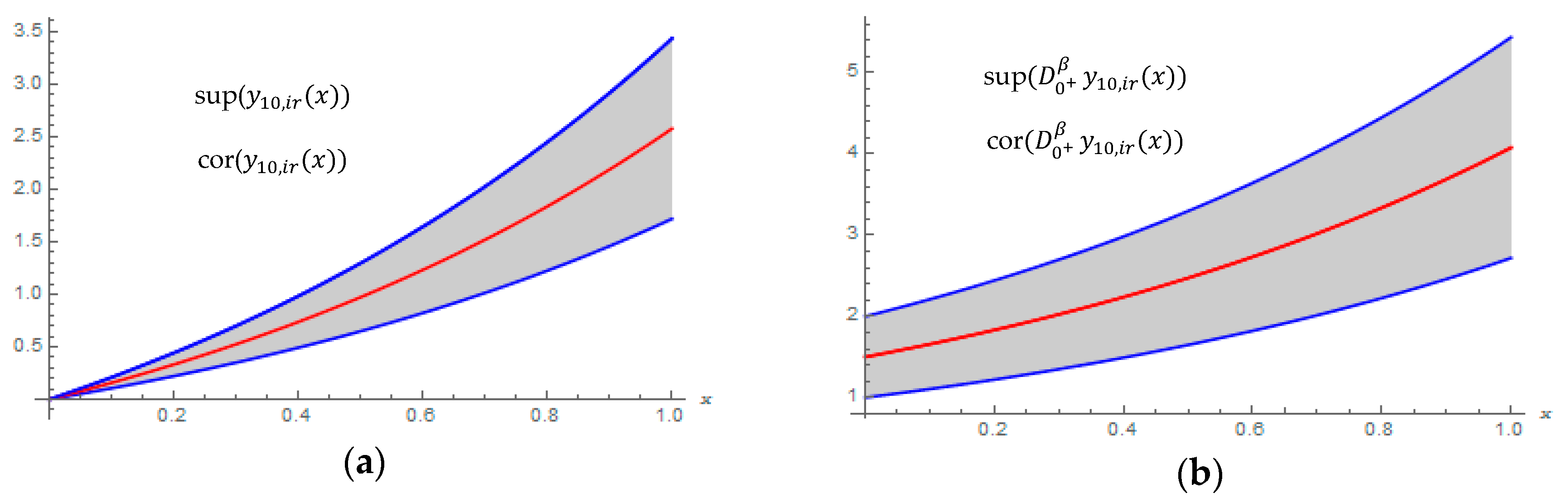
To show the fuzzy behavior of the proposed algorithm, the core and support of fuzzy ($m$)-approximated solutions, $m=1,2,$ and its Caputo derivative at $\beta =1$ of Example 1, are plotted in Figure 1 and Figure 2, where $core\left(y\left(x\right)\right)=\left\{\tau \in ℝ:y\left(x\right)\left(\tau \right)=1\right\}$, and $supp\left(y\left(x\right)\right)=\left\{\tau \in ℝ:y\left(x\right)\left(\tau \right)\ge 0\right\}$.

Figure 1. (a) The core and the support of fuzzy (1)-approximated solutions under Caputo [(1)-$\beta$]-differentiable; (b) The core and the support of derivative of fuzzy (1)-approximated solution under Caputo [(1)-$\beta$]-differentiable, at $\beta =1$ of Example 1: gray support and red core.

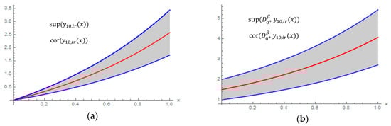
Figure 2. (a) The core and the support of fuzzy (2)-approximated solutions under Caputo [(2)-$\beta$]-differentiable; (b) The core and the support of fuzzy (2)-approximated Caputo derivatives solution under Caputo [(2)-$\beta$]-differentiable, at $\beta =1$ of Example 1: gray support and red core.

Example 2.

Consider the following FFIDE of Volterra type

$$D_{0^{+}}^{\beta }y\left(x\right)=\left[r-1, 1-r\right]+{\int }_0^{x}y\left(t\right)dt , 0<\beta \le 1, x\in \left[0,1\right],$$

(30)

with the fuzzy initial condition

$$y\left(0\right)=0.$$

(31)

Based on the type of differentiability, fuzzy FVIDEs (30) and (31) can be converted to one of the following systems:

Case 1: Under Caputo [(1)-$\beta$]-differentiability, the system of OFVIDEs corresponding to Caputo [(1)-$\beta$]-differentiable is

$$\begin{array}{c}{D}_{0^{+}}^{\beta }{y}_{1r}\left(x\right)=\left(r-1\right)+{\int }_0^x{y}_{1r}\left(t\right)dt,\\ D_{0^{+}}^{\beta }{y}_{2r}\left(x\right)=\left(1-r\right)+{\int }_0^x{y}_{2r}\left(t\right)dt,\end{array}$$

(32)

with the fuzzy initial condition

$$y_{1r}\left(0\right)=0,y_{2r}\left(0\right)=0.$$

(33)

If $\beta =1,$then the exact solution of OFVIDEs (32) and (33) is given by

$${\left[y\left(x\right)\right]}^r=\left[r-1, 1-r\right]sinh\left(x\right).$$

(34)

By utilizing the FRPS algorithm as presented previously, beginning with $y_{0,1r}=y_{1r}\left(0\right)=0, y_{0,2r}=y_{2r}\left(0\right)=0$, and depending on Equation (10), the $k$th-FRPS approximated solutions $y_{k,1r}\left(x\right)$ and $y_{k,2r}\left(x\right)$ for the system (32) and (33) are given by

$$\begin{array}{c}{y}_{k,1r}\left(x\right)={\sum }_{n=1}^k{c}_n\frac{x^{n\beta }}{\Gamma \left(n\beta +1\right)},\\ y_{k,2r}\left(x\right)={\sum }_{n=1}^k{d}_n\frac{x^{n\beta }}{\Gamma \left(n\beta +1\right)}.\end{array}$$

(35)

Consequently, the $k$th-residual functions $Re{s}_{k,1r},$ and $Re{s}_{k,2r}$ for (32) will be

$$\begin{array}{c}Re{s}_{k,1r}\left(x\right)=D_{0^{+} }^{\beta }{y}_{k,1r}\left(x\right)-{\int }_0^x{y}_{k,1r}\left(t\right)dt-\left(r-1\right),\\ Re{s}_{k,2r}\left(x\right)=D_{0^{+} }^{\beta }{y}_{k,2r}\left(x\right)-{\int }_0^x{y}_{k,2r}\left(t\right)dt-\left(1-r\right).\end{array}$$

(36)

The coefficients of the FRPS approximate solutions for the system (32) and (33) can be found in Appendix B.

Case 2: Under Caputo [(2)-$\beta$]-differentiability, the system of OFVIDEs corresponding to Caputo [(2)-$\beta$]-differentiable is

$$\begin{array}{c}{D}_{0^{+}}^{\beta }{y}_{1r}\left(x\right)=\left(1-r\right)+{\int }_0^x{y}_{2r}\left(t\right)dt,\\ D_{0^{+}}^{\beta }{y}_{2r}\left(x\right)=\left(r-1\right)+{\int }_0^x{y}_{1r}\left(t\right)dt,\end{array}$$

(37)

with the initial conditions

$$y_{1r}\left(0\right)=0, y_{2r}\left(0\right)=0.$$

(38)

If $\beta =1,$then the exact solutions of OFVIDEs (38) and (39) are given by

$${\left[y\left(x\right)\right]}^r=\left[1-r, r-1\right]\sin \left(x\right).$$

(39)

In view of the description for FRPS technique and starting with $y_{0,1r}=y_{1r}\left(0\right)=0,$ and $y_{0,2r}=y_{2r}\left(0\right)=0$, then the $k$th-residual functions of Equation (37) will be as follows

$$\begin{array}{c}Re{s}_{k,1r}\left(x\right)=D_{0^{+} }^{\beta }{y}_{k,1r}\left(x\right)-{\int }_0^x{y}_{k,2r}\left(t\right)dt-\left(1-r\right),\\ Re{s}_{k,2r}\left(x\right)=D_{0^{+} }^{\beta }{y}_{k,2r}\left(x\right)-{\int }_0^x{y}_{k,1r}\left(t\right)dt-\left(r-1\right).\end{array}$$

(40)

where $y_{k,1r}\left(x\right)$ and $y_{k,2r}\left(x\right)$ are given by

$$\begin{array}{c}{y}_{k,1r}\left(x\right)={\sum }_{n=1}^k{c}_n\frac{x^{n\beta }}{\Gamma \left(n\beta +1\right)},\\ y_{k,2r}\left(x\right)={\sum }_{n=1}^k{d}_n\frac{x^{n\beta }}{\Gamma \left(n\beta +1\right)}.\end{array}$$

(41)

The coefficients of the FRPS approximate solutions for the system (37) and (38) can be found in Appendix B.

To show the accuracy of the FRPS technique, numerical results for Example 2 at $n=10$, $r\in \left\{0.5,0.75\right\}$ with some selected grid points in $\left[0,1\right]$ are given in Table 5 and Table 6 with different values of $\beta$.

Table 5. Numerical results for Example 2, case 1, with different values of $\beta$.

${\mathit{y}}_{1\mathit{r}}\left(\mathit{x}\right)$
${\mathit{r}}_{\mathit{i}}$	${\mathit{x}}_{\mathit{i}}$	$\mathit{\beta }=1$	$\mathit{\beta }=0.9$	$\mathit{\beta }=0.8$	$\mathit{\beta }=0.7$
$0.5$	$0.2$	$-0.100668001$	$-0.123692685$	$-0.151695235$	$-0.186264438$
	$0.4$	$-0.205376163$	$-0.238161466$	$-0.277064940$	$-0.324760477$
	$0.6$	$-0.318326791$	$-0.359432909$	$-0.408753265$	$-0.470283639$
	$0.8$	$-0.444052990$	$-0.494515208$	$-0.556205023$	$-0.634532156$
$0.75$	$0.2$	$-0.050334001$	$-0.061846342$	$-0.075847617$	$-0.093132219$
	$0.4$	$-0.102688081$	$-0.119080733$	$-0.138532470$	$-0.162380238$
	$0.6$	$-0.159163396$	$-0.179716454$	$-0.204376633$	$-0.235141819$
	$0.8$	$-0.222026495$	$-0.247257604$	$-0.278102512$	$-0.317266078$
${\mathit{y}}_{2\mathit{r}}\left(\mathit{x}\right)$
${\mathit{r}}_{\mathit{i}}$	${\mathit{x}}_{\mathit{i}}$	$\mathit{\beta }=1$	$\mathit{\beta }=0.9$	$\mathit{\beta }=0.8$	$\mathit{\beta }=0.7$
$0.5$	$0.2$	$0.100668001$	$0.123692685$	$0.151695235$	$0.186264438$
	$0.4$	$0.205376163$	$0.238161466$	$0.277064940$	$0.324760477$
	$0.6$	$0.318326791$	$0.359432909$	$0.408753265$	$0.470283639$
	$0.8$	$0.444052990$	$0.494515208$	$0.556205023$	$0.634532156$
$0.75$	$0.2$	$0.050334001$	$0.061846342$	$0.075847617$	$0.093132219$
	$0.4$	$0.102688081$	$0.119080733$	$0.138532470$	$0.162380238$
	$0.6$	$0.159163396$	$0.179716454$	$0.204376633$	$0.235141819$
	$0.8$	$0.222026495$	$0.247257604$	$0.278102512$	$0.317266078$

Table 6. Numerical results for Example 2, case 2, with different values of $\beta$.

${\mathit{y}}_{1\mathit{r}}\left(\mathit{x}\right)$
${\mathit{r}}_{\mathit{i}}$	${\mathit{x}}_{\mathit{i}}$	$\mathit{\beta }=1$	$\mathit{\beta }=0.9$	$\mathit{\beta }=0.8$	$\mathit{\beta }=0.7$
$0.5$	$0.2$	$0.099334665$	$0.120583966$	$0.144646654$	$0.170765057$
	$0.4$	$0.194709171$	$0.217958708$	$0.239847027$	$0.258218270$
	$0.6$	$0.282321238$	$0.299033752$	$0.310147377$	$0.313819870$
	$0.8$	$0.358678047$	$0.363060372$	$0.359026685$	$0.346425845$
$0.75$	$0.2$	$0.049667333$	$0.060291983$	$0.072323327$	$0.085382529$
	$0.4$	$0.097354586$	$0.108979354$	$0.119923514$	$0.129109135$
	$0.6$	$0.141160618$	$0.149516876$	$0.155073688$	$0.156909935$
	$0.8$	$0.179339023$	$0.181530186$	$0.179513342$	$0.173212923$
${\mathit{y}}_{2\mathit{r}}\left(\mathit{x}\right)$
${\mathit{r}}_{\mathit{i}}$	${\mathit{x}}_{\mathit{i}}$	$\mathit{\beta }=1$	$\mathit{\beta }=0.9$	$\mathit{\beta }=0.8$	$\mathit{\beta }=0.7$
$0.5$	$0.2$	$-0.099334665$	$-0.120583966$	$-0.144646654$	$-0.170765057$
	$0.4$	$-0.194709171$	$-0.217958708$	$-0.239847027$	$-0.258218270$
	$0.6$	$-0.282321238$	$-0.299033752$	$-0.310147377$	$-0.313819870$
	$0.8$	$-0.358678047$	$-0.363060372$	$-0.359026685$	$-0.346425845$
$0.75$	$0.2$	$-0.049667333$	$-0.060291983$	$-0.072323327$	$-0.085382529$
	$0.4$	$-0.097354586$	$-0.108979354$	$-0.119923514$	$-0.129109135$
	$0.6$	$-0.141160618$	$-0.149516876$	$-0.155073688$	$-0.156909935$
	$0.8$	$-0.179339023$	$-0.181530186$	$-0.179513342$	$-0.173212923$

For the purpose of comparison, the absolute errors of $y_{1r}\left(x\right)$ and $y_{2r}\left(x\right)$ of Example 2, case 1, by using the FRPS method and Haar Wavelet (HW) method [35], for $n=8$, with fixed value of $\beta =1$ are given in Table 7. From this table, it can be observed that our method provides us with accurate approximated solutions to OFVIDEs (32) and (33).

Table 7. Comparisons of absolute errors of Example 2, case 1.

${\mathit{y}}_{1\mathit{r}}\left(\mathit{x}\right)$
${\mathit{x}}_{\mathit{i}}$	FRPS Method	HW Method
$0.1$	$2.76167\times {10}^{-15}$	$4.205\times {10}^{-6}$
$0.2$	$1.41145\times {10}^{-12}$	$5.305\times {10}^{-6}$
$0.3$	$5.42854\times {10}^{-11}$	$2.07\times {10}^{-6}$
${\mathit{y}}_{2\mathit{r}}\left(\mathit{x}\right)$
${\mathit{x}}_{\mathit{i}}$	FRPS Method	HW Method
$0.1$	$2.76167\times {10}^{-15}$	$2.876\times {10}^{-6}$
$0.2$	$1.41145\times {10}^{-12}$	$1.836\times {10}^{-6}$
$0.3$	$5.42854\times {10}^{-11}$	$1.295\times {10}^{-6}$

¹ Results of HW method referred in [35].

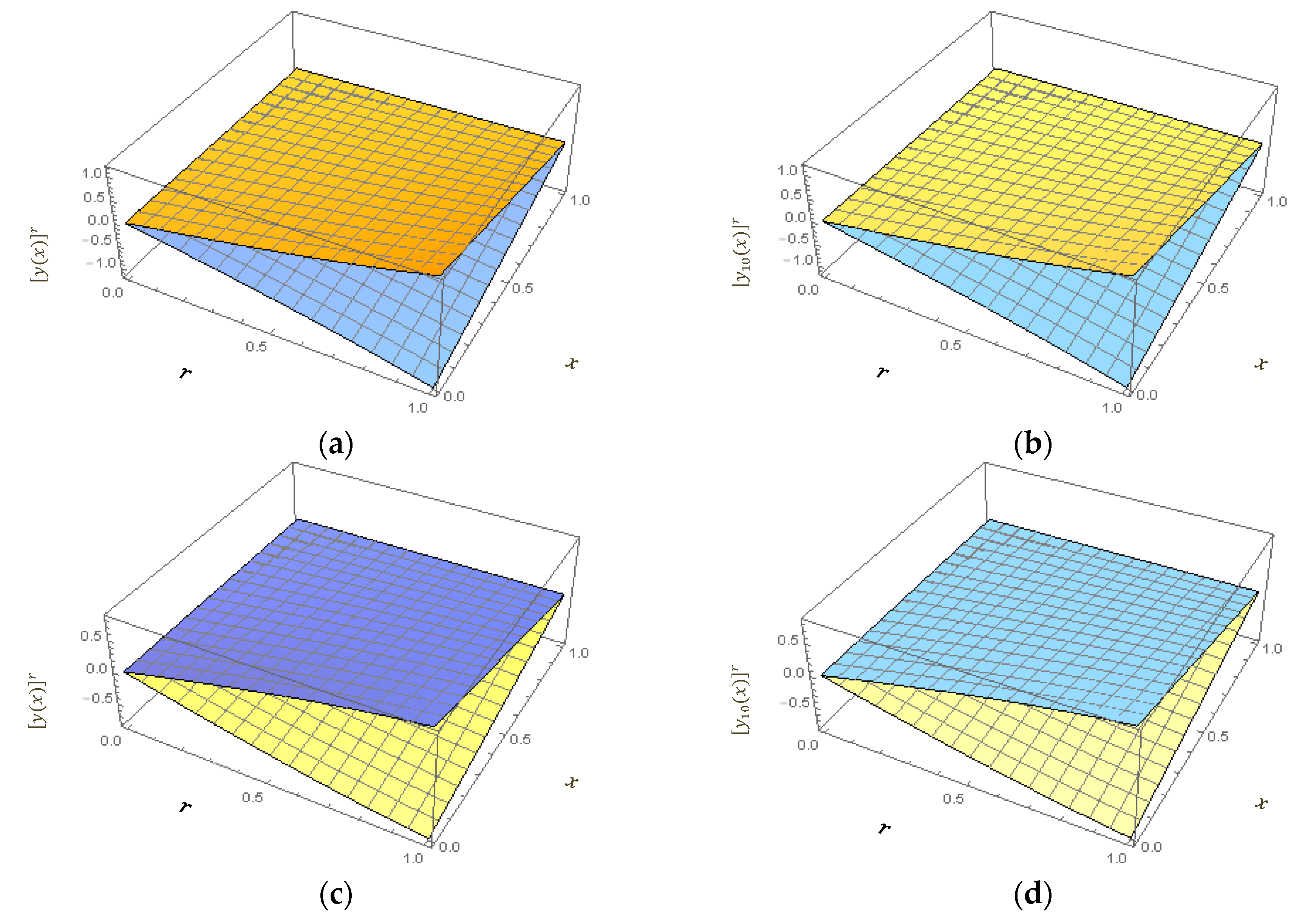
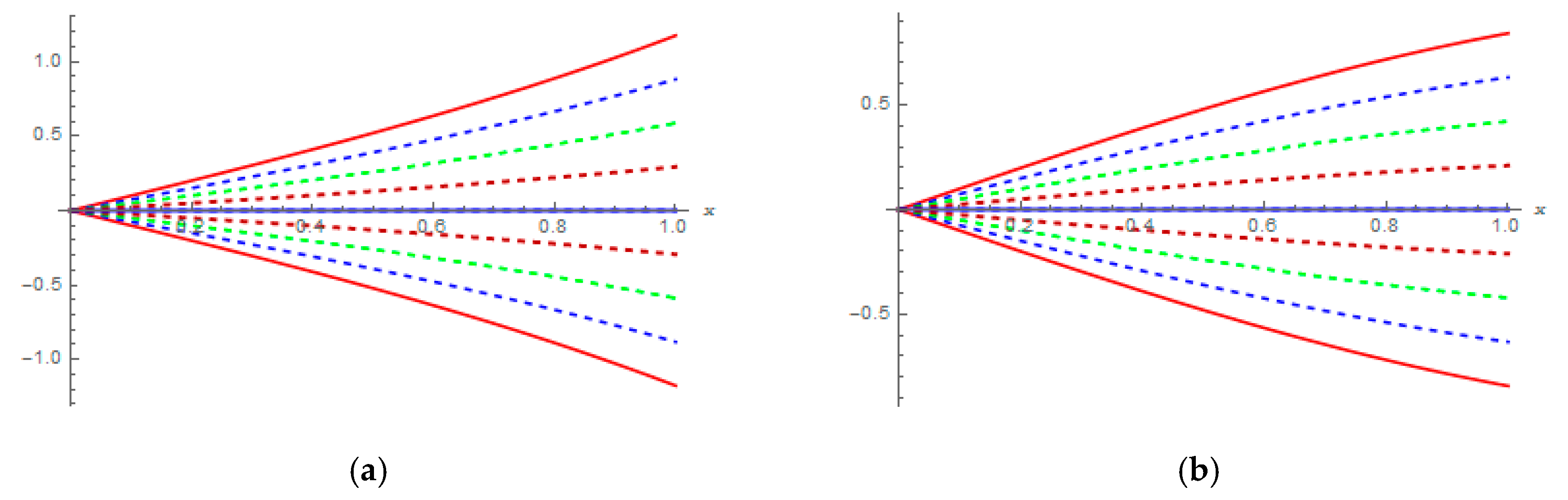
To show the fuzzy behavior of the proposed algorithm, the exact and 10th-FRPS approximated solutions of Example 2, case1 and case 2, are plotted in Figure 3. The plots of $r$-cut representation of exact and FRPS approximated solutions for Example 2, case 1 and case 2, are plotted in Figure 4 at $\beta =1$, $n=10$ and $r\in \left\{0,0.25,0.5,0.75,1\right\}$.

Figure 3. (a) Surface plot exact solution, case 1; (b) Surface plot of 10th-FRPS approximated solutions, case 1; (c) Surface plot exact solution, case 2; (d) Surface plot of 10th-FRPS approximated solutions, case 2, of Example 2 at $\beta =1$, for all $t\in \left[0,1\right]$ and $r\in \left[0,1\right]$: (yellow and blue are the upper and lower solution, respectively).

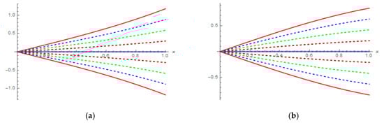
Figure 4. (a) Plots of $r$-cut representations of exact and ${\phi }_{10,1r}\left(t\right)$, of Example 2, case 1; (b) Plots of $r$-cut representations of exact and ${\phi }_{10,2r}\left(t\right)$, of Example 2, case 2, for $\beta =1,$ $t\in \left[0,1\right]$ with different values of $r$. in parametric form: red $r=0$, dashed blue $r=0.25$, dashed green $r=0.5$, darker red-dashed $r=0.75$, blue $r=1$.

6. Conclusions

In this paper, we have successfully used the FRPS technique to construct and investigate fuzzy approximated solutions for a class of fuzzy fractional Volterra integro-differential equations of order $0<\beta \le 1$, with appropriate fuzzy initial conditions under strongly generalized differentiability. This method is effectively applied without being exposed to any restriction such as conversion, discretization or perturbation. The methodology of the solution basically depends on constructing the residual function and employing the generalized Taylor formula under Caputo sense. Two illustrative examples are given to validate the capability and performance of our algorithm. The numerical results obtained via FRPS algorithm have shown that this technique is an easy, powerful tool which can effectively solve different types of fuzzy fractional integro-differential equations.

References

- Zhang, H.; Liao, X.; Yu, J. Fuzzy modeling and synchronization of hyperchaotic systems. Chaos Solitons Fractals 2005, 26, 835–843. [Google Scholar] [CrossRef]
- El Naschie, M.S. From experimental quantum optics to quantum gravity via a fuzzy Kähler manifold. Chaos Solitons Fractals 2005, 25, 969–977. [Google Scholar] [CrossRef]
- Diamond, P. Time-dependent differential inclusions, cocycle attractors and fuzzy differential equations. IEEE Trans. Fuzzy Syst. 1999, 7, 734–740. [Google Scholar] [CrossRef]
- Feng, G.; Chen, G. Adaptive control of discrete time chaotic systems: a fuzzy control approach. Chaos Solitons Fractals 2005, 23, 459–467. [Google Scholar] [CrossRef]
- Priyadharsini, S.; Parthiban, V.; Manivannan, A. Solution of fractional integro-differential system with fuzzy initial condition. Int. J. Pure Appl. Math. 2016, 106, 107–112. [Google Scholar]
- Shabestari, M.R.; Ezzati, R.; Allahviranloo, T. Numerical solution of fuzzy fractional integro-differential equation via two-dimensional Legendre wavelet method. J. Intell. Fuzzy Syst. 2018, 34, 2453–2465. [Google Scholar] [CrossRef]
- Padmapriya, V.; Kaliyappan, M.; Parthiban, V. Solution of Fuzzy Fractional Integro-Differential Equations Using A Domian Decomposition Method. J. Inform. Math. Sci. 2017, 9, 501–507. [Google Scholar]
- Matinfar, M.; Ghanbari, M.; Nuraei, R. Numerical solution of linear fuzzy Volterra integro-differential equations by variational iteration method. J. Intell. Fuzzy Syst. 2013, 24, 575–586. [Google Scholar]
- Gumah, G.; Moaddy, K.; Al-Smadi, M.; Hashim, I. Solutions to uncertain Volterra integral equations by fitted reproducing kernel Hilbert space method. J. Funct. Spaces 2016, 2016, 2920463. [Google Scholar] [CrossRef]
- Alikhani, R.; Bahrami, F. Global solutions for nonlinear fuzzy fractional integral and integrodifferential equations. Commun. Nonlinear Sci. Numer. Siml. 2013, 18, 2007–2017. [Google Scholar] [CrossRef]
- Saadeh, R.; Al-Smadi, M.; Gumah, G.; Khalil, H.; Khan, R.A. Numerical Investigation for Solving Two-Point Fuzzy Boundary Value Problems by Reproducing Kernel Approach. Appl. Math. Inf. Sci. 2016, 10, 1–13. [Google Scholar] [CrossRef]
- Gumah, G.N.; Naser, M.F.M.; Al-Smadi, M.; Al-Omari, S.K. Application of reproducing kernel Hilbert space method for solving second-order fuzzy Volterra integro-differential equations. Adv. Diff. Equ. 2018, 2018, 475. [Google Scholar] [CrossRef]
- Salahshour, S.; Allahviranloo, T.; Abbasbandy, S. Solving fuzzy fractional differential equations by fuzzy Laplace transforms. Commun. Nonlinear Sci. Numer. Siml. 2012, 17, 1372–1381. [Google Scholar] [CrossRef]
- Abu Arqub, O.; Momani, S.; Al-Mezel, S.; Kutbi, M. Existence, uniqueness, and characterization theorems for nonlinear fuzzy integrodifferential equations of Volterra type. Math. Probl. Eng. 2015, 2015, 835891. [Google Scholar] [CrossRef]
- Al-Smadi, M.; Abu Arqub, O. Computational algorithm for solving fredholm time-fractional partial integrodifferential equations of dirichlet functions type with error estimates. Appl. Math. Comput. 2019, 342, 280–294. [Google Scholar] [CrossRef]
- Abu Arqub, O.; Odibat, Z.; Al-Smadi, M. Numerical solutions of time-fractional partial integrodifferential equations of Robin functions types in Hilbert space with error bounds and error estimates. Nonlinear Dyn. 2018, 94, 1819–1834. [Google Scholar] [CrossRef]
- Abu Arqub, O.; Al-Smadi, M. Numerical algorithm for solving time-fractional partial integrodifferential equations subject to initial and Dirichlet boundary conditions. Num. Methods Partial Diff. Equ. 2018, 34, 1577–1597. [Google Scholar] [CrossRef]
- Abu Arqub, O.; Al-Smadi, M. Numerical algorithm for solving two-point, second-order periodic boundary value problems for mixed integro-differential equations. Appl. Math. Comput. 2014, 243, 911–922. [Google Scholar] [CrossRef]
- Abu Arqub, O. Series solution of fuzzy differential equations under strongly generalized differentiability. J. Adv. Res. Appl. Math. 2013, 5, 31–52. [Google Scholar] [CrossRef]
- Moaddy, K.; Al-Smadi, M.; Hashim, I. A novel representation of the exact solution for differential algebraic equations system using residual power-series method. Discrete Dyn. Nat. Soc. 2015, 2015, 205207. [Google Scholar] [CrossRef]
- El-Ajou, A.; Abu Arqub, O.; Momani, S.; Baleanu, D.; Alsaedi, A. A novel expansion iterative method for solving linear partial differential equations of fractional order. Int. J. Appl. Math. Comput. 2015, 257, 119–133. [Google Scholar] [CrossRef]
- Elajou, A.; Abu Arqub, O.; Zhour, Z.A. New Results on Fractional Power Series: Theory and Applications. Entropy 2013, 12, 5305–5323. [Google Scholar] [CrossRef]
- Komashynska, I.; Al-Smadi, M.; Abu Arqub, O.; Momani, S. An efficient analytical method for solving singular initial value problems of nonlinear systems. Appl. Math. Inf. Sci. 2016, 10, 647–656. [Google Scholar] [CrossRef]
- Komashynska, I.; Al-Smadi, M.; Ateiwi, A.; Al-Obaidy, S. Approximate analytical solution by residual power series method for system of Fredholm integral equations. Appl. Math. Inf. Sci. 2016, 10, 1–11. [Google Scholar] [CrossRef]
- El-Ajou, A.; Abu Arqub, O.; Al-Smadi, M. A general form of the generalized Taylor’s formula with some applications. Appl. Math. Comput. 2015, 256, 851–859. [Google Scholar] [CrossRef]
- Alaroud, M.; Al-Smadi, M.; Ahmad, R.R.; Din, S.K.U. Computational optimization of residual power series algorithm for certain classes of fuzzy fractional differential equations. Int. J. Differ. Equ. 2018, 2018, 8686502. [Google Scholar] [CrossRef]
- Moaddy, K.; Al-Smadi, M.; Abu Arqub, O.; Hashim, I. Analytic-numeric treatment for handling system of second-order, three-point BVPs. In Proceedings of the AIP Conference, Seoul, Korea, 23–27 May 2017; Volume 1830, p. 020025. [Google Scholar]
- Kaleva, O. Fuzzy differential equations. Fuzzy Sets Syst. 1987, 24, 301–317. [Google Scholar] [CrossRef]
- Goetschel, J.R.; Voxman, W. Elementary fuzzy calculus. Fuzzy Sets Syst. 1986, 18, 31–43. [Google Scholar] [CrossRef]
- Puri, M.L.; Ralescu, D.A. Differentials of fuzzy functions. J. Math. Anal. Appl. 1983, 91, 552–558. [Google Scholar] [CrossRef]
- Bede, B.; Gal, S.G. Generalizations of the differentiability of fuzzy-number-valued functions with applications to fuzzy differential equations. Fuzzy Sets Syst. 2005, 151, 581–599. [Google Scholar] [CrossRef]
- Moaddy, K.; Freihat, A.; Al-Smadi, M.; Abuteen, E.; Hashim, I. Numerical investigation for handling fractional-order Rabinovich–Fabrikant model using the multistep approach. Soft Comput. 2018, 22, 773–782. [Google Scholar] [CrossRef]
- Chalco-Cano, Y.; Roman-Flores, H. On new solutions of fuzzy differential equations. Chaos Solitons Fractals 2008, 38, 112–119. [Google Scholar] [CrossRef]
- Salahshour, S.; Allahviranloo, T.; Abbasbandy, S.; Baleanu, D. Existence and uniqueness results for fractional differential equations with uncertainty. Adv. Differ. Equ. 2012, 1, 112. [Google Scholar] [CrossRef]
- Ali, M.R. Approximate solutions for fuzzy Volterra integrodifferential equations. J. Abst. Comput. Math. 2018, 3, 11–22. [Google Scholar]
© 2019 by the authors. Licensee MDPI, Basel, Switzerland. This article is an open access article distributed under the terms and conditions of the Creative Commons Attribution (CC BY) license (http://creativecommons.org/licenses/by/4.0/).