Article

Clustering Mixed Data Based on Density Peaks and Stacked Denoising Autoencoders

1
College of Computer and Information, Hohai University, Nanjing 211100, China
2
Department of Mathematics and Physics, Hefei University, Hefei 230601, China
3
College of Computer Science and Technology, HuaiBei Normal University, HuaiBei 235000, China
4
Jiangsu Provincial Key Constructive Laboratory for Big Data of Psychology and Cognitive Science, Yancheng Teachers University, Yancheng 224002, China
*
Author to whom correspondence should be addressed.
Symmetry 2019, 11(2), 163; https://doi.org/10.3390/sym11020163
Submission received: 10 January 2019 / Revised: 23 January 2019 / Accepted: 26 January 2019 / Published: 1 February 2019

Abstract

:
With the universal existence of mixed data with numerical and categorical attributes in real world, a variety of clustering algorithms have been developed to discover the potential information hidden in mixed data. Most existing clustering algorithms often compute the distances or similarities between data objects based on original data, which may cause the instability of clustering results because of noise. In this paper, a clustering framework is proposed to explore the grouping structure of the mixed data. First, the transformed categorical attributes by one-hot encoding technique and normalized numerical attributes are input to a stacked denoising autoencoders to learn the internal feature representations. Secondly, based on these feature representations, all the distances between data objects in feature space can be calculated and the local density and relative distance of each data object can be also computed. Thirdly, the density peaks clustering algorithm is improved and employed to allocate all the data objects into different clusters. Finally, experiments conducted on some UCI datasets have demonstrated that our proposed algorithm for clustering mixed data outperforms three baseline algorithms in terms of the clustering accuracy and the rand index.

1. Introduction

Clustering analysis, an important unsupervised data analysis and data mining approaches, has been studied extensively and applied successfully to various domains, such as gene expression analysis [1,2], fraud detection [3], imagine segmentation [4], and document mining [5,6]. The basic clustering algorithms mainly group data objects into different clusters based on the similarities between objects in original data space, making objects in the same cluster are more similar while those in different clusters are more dissimilar. Many traditional clustering approaches, such as k-means [7], DBSCAN [8], spectral clustering [9,10], can only handle datasets with numerical attributes. However, the partition of mixed data objects with both categorical attributes and numerical attributes is indispensable in various fields, such as economics, finance, politics, and clinical medicine. In these cases, we need to consider simultaneously numerical attributes and categorical attributes, which provide more useful information and are helpful to find the potential grouping structure. For example, Italian local labor market areas can be identified by employing a min-cut approach based on iterative partitioning of the transitions graph [11]. Patients with heart disease can be recognized by analyzing various features consisting of categorical attributes and numerical attributes. Bank credit officers can decide to approve or reject the credit card applications depending on the mixed attribute values of credit card applicants. In these practical applications, it is crucial that how to transform categorical attributes into numerical values with keeping useful information as much as possible. In order to conduct clustering the mixed data better, more and more clustering algorithms have been proposed, such as k-prototypes [12], OCIL [13], DP-MD-FN [14], and so on.
A simple approach to clustering mixed data is transformation-based method, which converts one type of attribute values to other type ones, then employs corresponding clustering algorithms for single type of attributes, such as conceptual k-means [15] and DSqueezer [16]. The most popular and classical partition-based clustering algorithm for mixed data was k-prototypes proposed by Huang [12], which was the integration of k-means and k-modes [17]. The variants of k-prototypes, such as fuzzy k-prototype [18] and KL-FCM-GM [19], were presented to improve k-prototypes by addressing the uncertainty of mixed data. Density peaks clustering (referred to as DPC) [20] is an effective clustering algorithm based on local density and relative distance. In order to make DPC algorithm handle mixed data, some algorithms were proposed based on different types of unified similarity or dissimilarity metrics for numerical and categorical attributes, such as DP-MD-FN [14], DPC-MD [21], and DPC-M [22]. In recent years, deep learning has attracted more attention in various fields and many methods have been investigated by integrating deep neural networks and clustering algorithms on numerical data, such as DEC [23], DBC [24], and DNC [25].
However, two main limitations exist in the clustering algorithms above:
(1)
DPC-based clustering algorithms for mixed data, such as DP-MD-FN [14], DPC-MD [21], and DPC-M [22], need to select the number of cluster centers by decision graph manually as DPC.
(2)
Most of deep learning-based clustering algorithms, such as DEC [23], DBC [24], and DNC [25], are only suitable for clustering numerical data with spherical distribution due to integration of the deep learning and k-means algorithm.
Due to the sparsity and discontinuity of the original mixed data space, many traditional clustering approaches for mixed data based on the distance or similarity in original data space are hard to find the true grouping structure of mixed data objects, especially in context with noise. The aim of this paper is to construct a continuous feature space for mixed data and present a clustering framework named DPC-SDAE based on this feature space. Firstly, one-hot encoding technique is employed to transform categorical attribute values into numerical ones with keeping useful information as much as possible. Secondly, based on the transformed categorical attribute values and normalized numerical attribute values, stacked denoising autoencoders are used to extract feature representations robust to noise for mixed data to construct a continuous feature space. Finally, the improved density peaks clustering algorithm is employed to perform clustering mixed data objects based on the feature space, which is suitable for clustering data objects with nonspherical distribution effectively.
The main contributions of this paper can be summarized as follows.
(1)
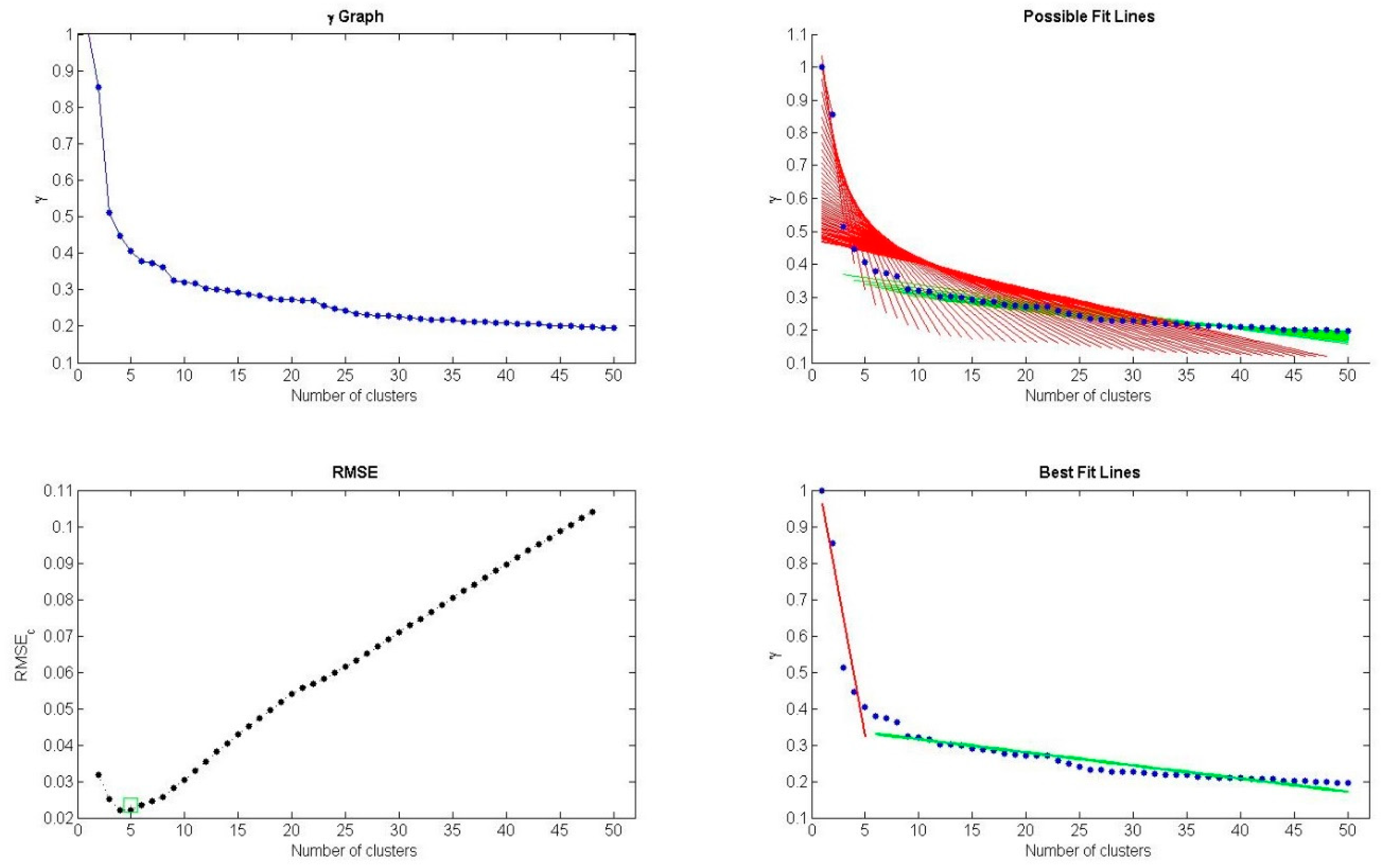
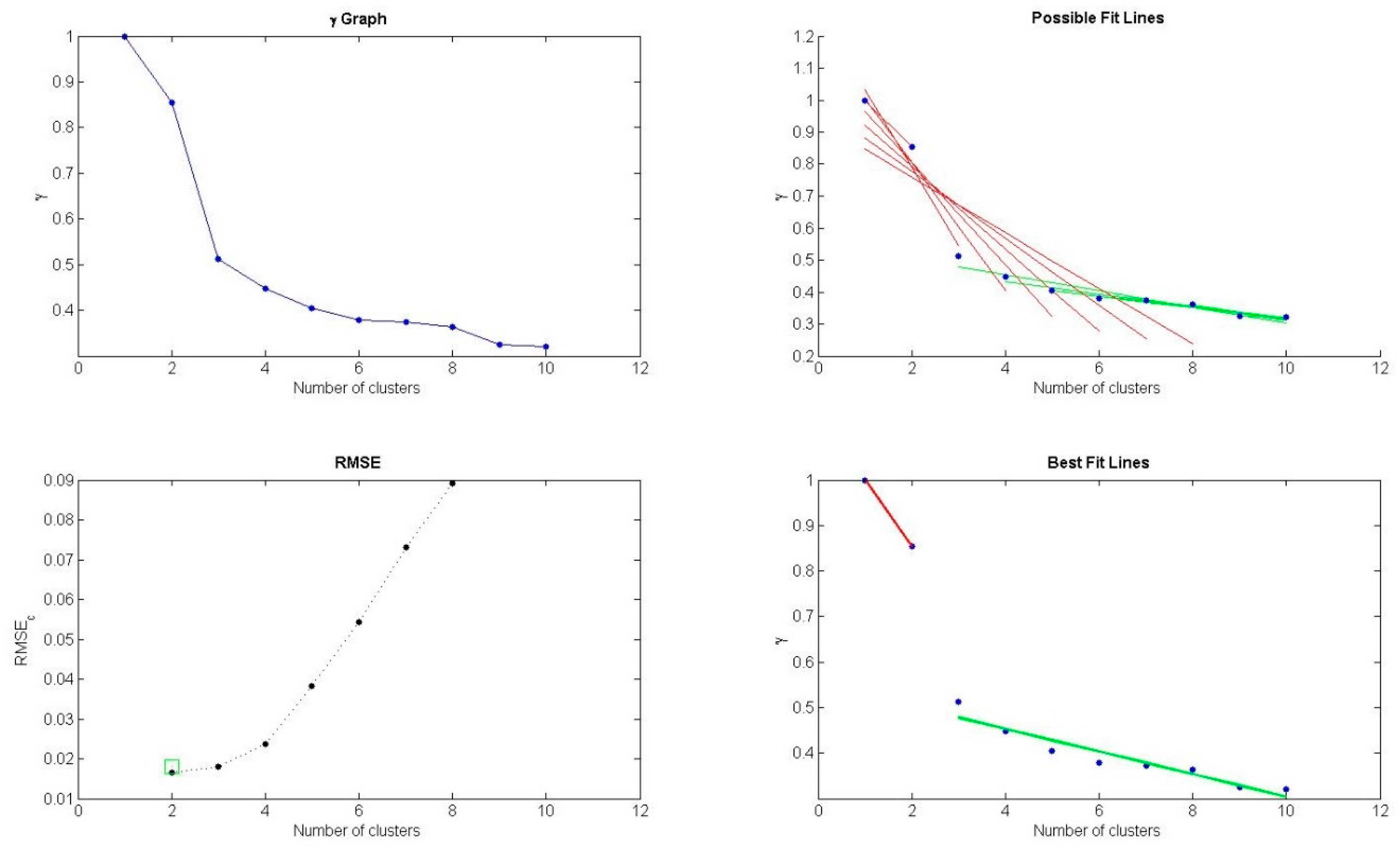
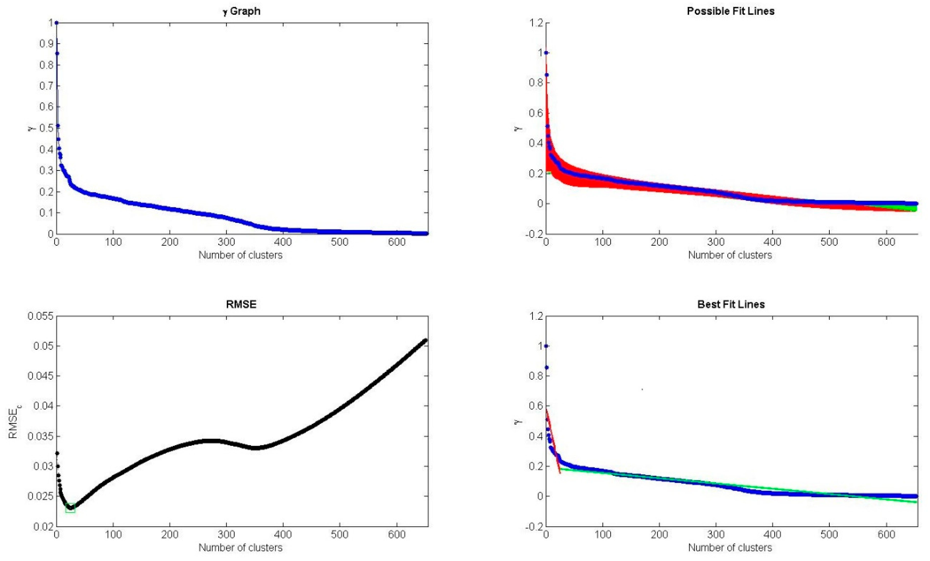
The DPC algorithm is improved by employing L-method to determine the number of cluster centers automatically, which overcomes the drawback of selecting the number of cluster centers by decision graph manually in DPC-based algorithms.
(2)
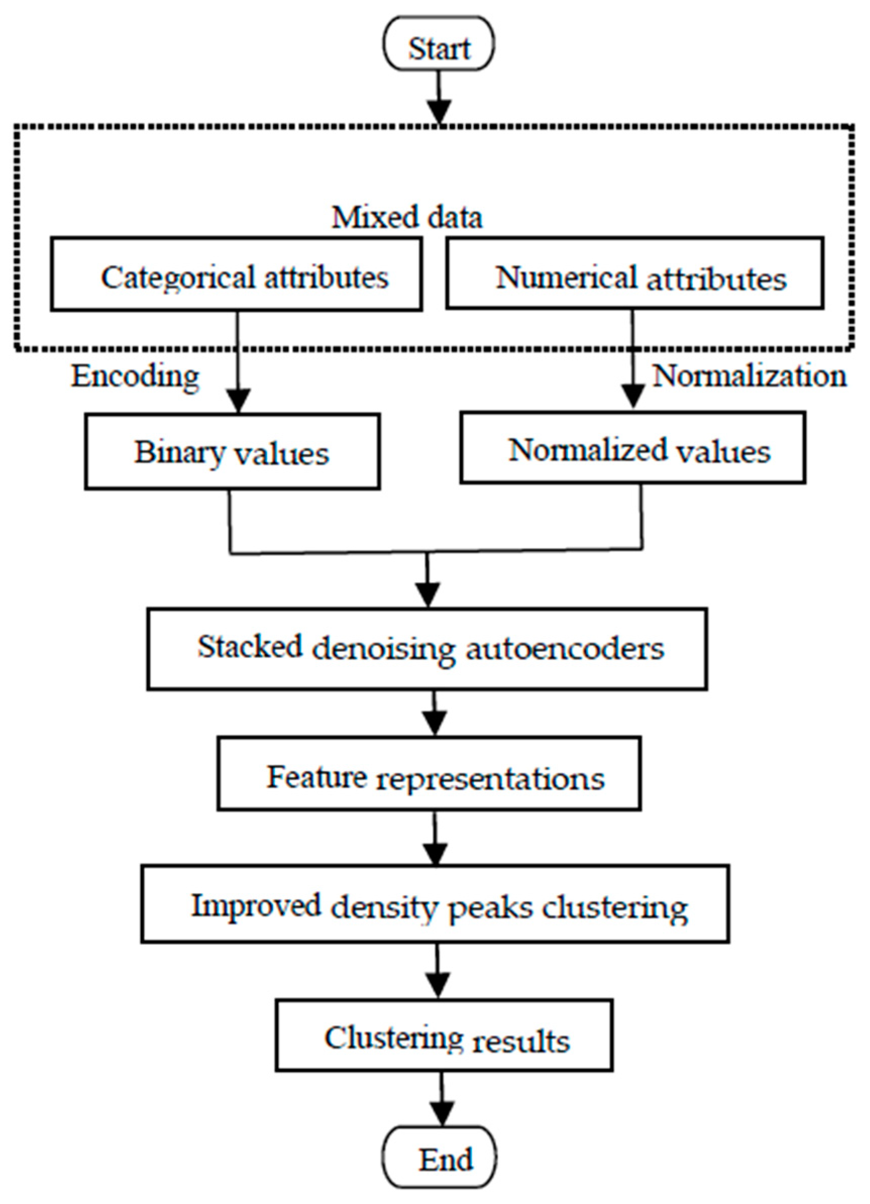
Based on numeralization of categorical attributes by the one-hot encoding technique, we propose a framework for clustering mixed data by integrating stacked denoising autoencoders and density peaks clustering algorithm, which can utilize the robust feature representations learned from SDAE to enhance the clustering quality and be also suitable for clustering data with nonspherical distribution based on density peaks clustering algorithm.
(3)
By conducting experiments on six datasets from UCI machine learning repository, we observed that our proposed clustering algorithm outperforms three baseline algorithms in terms of clustering accuracy and rand index, which also demonstrates that stacked denoising autoencoders can be applied to clustering small sample datasets effectively besides clustering large scale datasets.
The rest of this paper is organized as follows. In Section 2, some related works are reviewed. Section 3 describes our proposed methodology. The details of our experiments results and discussions are presented in Section 4, followed by a conclusion in Section 5.

2. Related Works

In this section, we mainly review related works on (1) clustering approaches to mixed data and (2) clustering algorithms based on deep learning. Based on analyzing the limitations of related works in detail, we present our DPC-SDAE clustering algorithm to address these limitations.

2.1. Clustering Approaches to Mixed Data

Most existing methods for clustering mixed data can be divided into three subsets—transformation-based clustering, partition-based clustering, and density-based clustering.
The transformation-based clustering method is the earliest type of clustering mixed data, which usually converts one type of attribute values to the other so that corresponding algorithms for clustering only single type data can be adopted. For example, H. Ralarbondrainy [15] encoded each categorical attribute value with a set of binary numerical values, then employed k-means algorithms to perform clustering analysis for mixed data on transformed categorical attributes and numerical attributes. To overcome the difficulty of measuring similarity degree of the above binary encoding, Hsu and Huang [26] proposed an incremental clustering method for mixed data based on distance hierarchy from domain knowledge. In addition, Zhang et al. [27] presented a method to transform categorical attributes into numerical representations through multiple transitive distance learning and embedding. In contrast, He et al. [16] presented the DSqueezer algorithm based on the discretization of all the numerical attributes, which could be utilized to cluster mixed data. Moreover, David and Averbuch [28] converted input data into categorical values according to the Calinski–Harabasz index and then reduced their dimensionalities in SpectralCAT, followed by spectral clustering algorithm conducted on. In general, either encoding categorical attributes into numerical ones or discretizing numerical attributes to categorical values may destroy the structure of original data space, inevitably causing loss of useful information, for instance, the difference between the values of each numerical attribute [29].
Different from transformation-based clustering algorithms, partition-based clustering algorithms attempt to group all the data objects into k clusters according to the unified distance of categorical and numerical attributes between each data object and each initialized cluster center firstly, where k is the preassigned number of clusters, and then they reallocate each data object to the cluster with its center nearest to the corresponding data object by an iterative way, until the partition remains unchanged or reaches the predefined maximum number of iterations. The most popular and classical partition-based clustering algorithm for mixed data is k-prototypes [12], presented by Huang in 1997, which is the integration of k-means for clustering numerical data and k-modes [17] for clustering categorical data. It mixes the means of numeric attributes and the modes of categorical attributes as the prototypes, then obtains the clustering results by alternatively updating the prototypes and group allocations of each data object based on a unified distance. This unified distance is a weighted distance of Euclidean distance for numerical attributes and Hamming distance for categorical attributes. To take into account the uncertainty of mixed data, Ji et al. proposed a fuzzy k-prototype clustering algorithm [18], which represented the prototype of a cluster with the integration of mean and fuzzy centroid, and improved the k-prototype algorithm based on a dissimilarity measure considering the significance of each attribute. To overcome convergence to the local optimum of k-prototype clustering algorithm, an evolutionary k-prototype (EKP) algorithm [30] was put forward to conduct clustering for mixed data with a framework of integrating evolutionary algorithm with k-prototype algorithm. Extensive experiments performed with the k-prototype algorithm and its variants have demonstrated that clustering results are determined greatly on the parameter γ, which is utilized to balance the importance degree of numerical attributes and categorical attributes. Nevertheless, determining an appropriate value of the parameter γ is a very tricky task for a common user. Instead of adjusting the attribute importance of different types by a parameter, Cheung and Jia [13] developed a parameter-free iterative clustering algorithm based on the concept of object-cluster similarity (OCIL), which adopted a unified similarity metric to conduct the clustering of mixed data. The KL-FCM-GM algorithm [19] provided a fuzzy c-means (FCM) type algorithm for clustering mixed data by constructing a fully probabilistic dissimilarity functional. In general, most of partition-based clustering algorithms are sensitive to the initial centroids or prototypes and only suitable for clustering mixed data with spherical distribution.
To circumvent the above problems of partition-based clustering algorithms, a wide variety of density-based algorithms are proposed to handle the clustering analysis of mixed data with nonspherical distribution. For example, EPDCA [31] extended DBSCAN [8], a well-known density-based clustering algorithm for numerical data, to cluster mixed data with integration of entropy and probability distribution. To address the difficulty of parameter specification in density-based clustering algorithms, Behzadi et al. [32] proposed a parameter-free modified DBSCAN clustering algorithm (MDBSCAN) for mixed data, which employed distance hierarchy and minimum description length. Density peaks clustering (referred to as DPC) [20] proposed by Rodriguez and Laio is an effective clustering algorithm based on local density and relative distance. The main idea of DPC algorithm is that the data objects with higher local density and being farther from other objects with a higher local density are chosen as cluster centers, followed by assigning each remaining data object to the same cluster as its nearest cluster center. To make DPC algorithm be applicable for clustering mixed data, DP-MD-FN [14] combined an entropy-based strategy with DPC and employed fuzzy neighborhood to calculate the local density-based on a uniform similarity measure. In addition, some researchers extended DPC by defining other different types of unified similarity or dissimilarity metrics to handle numerical and categorical attributes simultaneously, such as DPC-MD [21] and DPC-M [22]. However, any unified similarity or dissimilarity metric may not be effective for all mixed datasets, and defining a proper unified similarity or dissimilarity metric for a given dataset is not an easy task.

2.2. Clustering Algorithm Based on Deep Learning

With the development of deep learning technology, a variety of deep neural networks are applied to clustering analysis so as to improve the effect of clustering. For example, deep embedded clustering (DEC) [23] employed stacked denoising autoencoders [33] to extract clustering-oriented representations and iteratively refined clusters with an auxiliary target distribution, optimizing both feature representations and cluster assignments simultaneously. Discriminatively boosted clustering (DBC) [24] used a fully convolutional autoencoder to extract coarse image features, and then conducted a discriminatively boosted clustering with learned features and soft k-means. Clustering convolutional neural network (CCNN) [34] leveraged a convolutional neural network (CNN) to perform large-scale image clustering by optimizing cluster centroid updating and representation learning iteratively with stochastic gradient descent approach. Deep nonparametric clustering (DNC) [25] proposed a unified framework of learning unsupervised features by employing deep belief network (DBN) and nonparametric clustering with maximum margin. In recent years, deep generative models and their applications have become a hot topic in machine learning and pattern recognition, attracting the extensive interest of researchers. Among of them, variational autoencoder (VAE) [35] and generative adversarial network (GAN) [36] are the two most prominent models for classification tasks. Variational deep embedding (VaDE) [37] generalized VAE to perform clustering tasks by a mixture of Gaussians prior instead of the single Gaussian prior. Information maximizing generative adversarial network (InfoGAN) [38] was presented to cluster data based on adding an information-theoretic regularization to the optimizing objective of standard GAN. An unsupervised feature learning (UFL) with fuzzy ART (UFLA) [39] was proposed to perform clustering on the mixed data. A high-order k-means algorithm was proposed based on dropout deep learning models for heterogeneous data clustering in cyber–physical–social systems [40]. To save space of this paper, more details related to clustering algorithms based on deep learning can be found in [41,42]. Although clustering methods based on deep generative models can achieve more satisfactory effect by generating more samples to extract robust representations, they are not suitable for clustering large-scale data due to their high computation complexity. In general, most of existing clustering approaches based on deep learning are designed for clustering numerical data by employing partition-based clustering algorithms, which are only suitable for data with spherical distribution.
To overcome the limitations of clustering algorithms above, this paper propose an algorithm framework named DPC-SDAE for clustering mixed data by integrating stacked denoising autoencoders with density peaks clustering, which can utilize the robust feature representations learned from SDAE and the capability of clustering data with any distribution of density peaks clustering to enhance the clustering quality.

3. Methodology

In this section, we introduce our proposed algorithm for clustering mixed data in detail. First of all, our overall framework of DPC-SDAE is shown in Figure 1, then, the data preprocessing procedure is introduced, followed by extracting features by a stacked denoising autoencoders (SDAE). In addition, we improve density peaks clustering by utilizing an L-method to determine the number of cluster centers automatically. Finally, the proposed DPC-SDAE algorithm is summarized and its time complexity is analyzed.
As illustrated in Figure 1, the categorical attributes of mixed data are encoded into binary values by one-hot encoding technique, and the numerical attributes of mixed data are transformed to the normalized values using a min–max normalization technique. Then, the transformed values are input to the stacked denoising autoencoders to learn useful and robust feature representations. Based on these feature representations, the original mixed data can be clustered by our improved density peaks clustering algorithm to obtain corresponding clustering results, i.e., group data objects into corresponding subsets.

3.1. Data Prepocessing

Let X = { x 1 , x 2 , , x N } denote a dataset consisting of N objects and x i = ( x i , 1 c , x i , 2 c , , x i , p c , x i , p + 1 r , x i , p + 2 r , , x i , m r ) be the ith data object represented by p categorical attribute values x i , 1 c , x i , 2 c , , x i , p c and m p numerical attribute values x i , p + 1 r , x i , p + 2 r , , x i , m r for 1 i N .
To facilitate extracting useful feature representations from original mixed data by stacked denoising autoencoders, we should transform categorical attribute values into binary numerical ones and normalize numerical attribute values at first.

3.1.1. Encoding of Categorical Attributes

As a simple and effective encoding technique, one-hot encoding is the most popular approach to handling numeralization of categorical attributes [43]. It can convert each value of categorical attributes to a binary vector, whose element with value 1 is only one, the others are zeros. The element with value 1 indicates the presence of corresponding possible value of a categorical attribute. For example, assuming that the categorical attribute color has only three possible values—e.g., red, green, and blue—with one-hot encoding, the red can be encoded to ( 1 , 0 , 0 ) , the green can be converted to ( 0 , 1 , 0 ) , while the blue can be transformed into ( 0 , 0 , 1 ) .
The jth categorical attribute A j ( 1 j p ) with n j possible values, can be encoded by a one-hot encoding mapping, as illustrated in (1).
f j c :   A j B n j
where B n j denotes a set containing binary vectors with n j dimensionality and each element is composed of a single one and n j 1 zeros.
After one hot encoding, the jth categorical attribute value x i , j c of the ith data object will be transformed into a binary row vector z i , j with n j dimensionality, where z i , j = f j c ( x i , j c ) . By combining the encoding vectors z 1 , j , z 2 , j , , z N , j of N objects of a categorical attribute A j ( 1 j p ) from top to bottom, we can get a N × n j matrix Z j . Finally, we concatenate Z 1 , Z 2 , , Z p to a N × j = 1 p n j matrix Z = [ Z 1 , Z 2 , , Z p ] , which can be viewed as the encoded matrix of all categorical attribute values of original dataset.

3.1.2. Normalization of Numerical Attributes

Usually, different numerical attributes have different magnitudes or units, which may greatly affect the value of similarity or dissimilarity between two distinct data objects. The larger the magnitude of a numerical attribute is, the more the attribute contributes to the similarity or dissimilarity between two data objects. To eliminate the effect of discrepancy in magnitude between different numerical attributes, numerical attribute values should be normalized. One of popular normalization methods is min–max normalization, which can linearly transform each numerical attribute value into a value between 0 and 1.
For a numerical attribute A j ( p + 1 j m ) , the jth attribute value x i , j r of the ith data object x i can be normalized by min–max normalization, as shown in (2).
y i , j r = x i , j r x min , j r x max , j r x min , j r
where, y i , j r denotes the normalized numerical attribute value of x i , j r , x max , j r and x min , j r represent the maximum and minimum value of numerical attribute A j among all the data objects, respectively.
After normalization of numerical attribute values of N objects, we can arrange all the normalized values into a N × ( m p ) matrix Y = [ y i , j r ] N × ( m p ) , which represents the normalized matrix of all numerical attribute values of original dataset.
Let D = [ Z , Y ] = ( d 1 , d 2 , , d N ) T denotes the transformed data matrix with the size of N × ( m p + j = 1 p n j ) , which d i ( 1 i N ) refers to the transformed attribute vector of the ith data object. The transformed attribute vectors of all data objects can input to stacked denoising autoencoders to extract feature representations instead of original dataset.

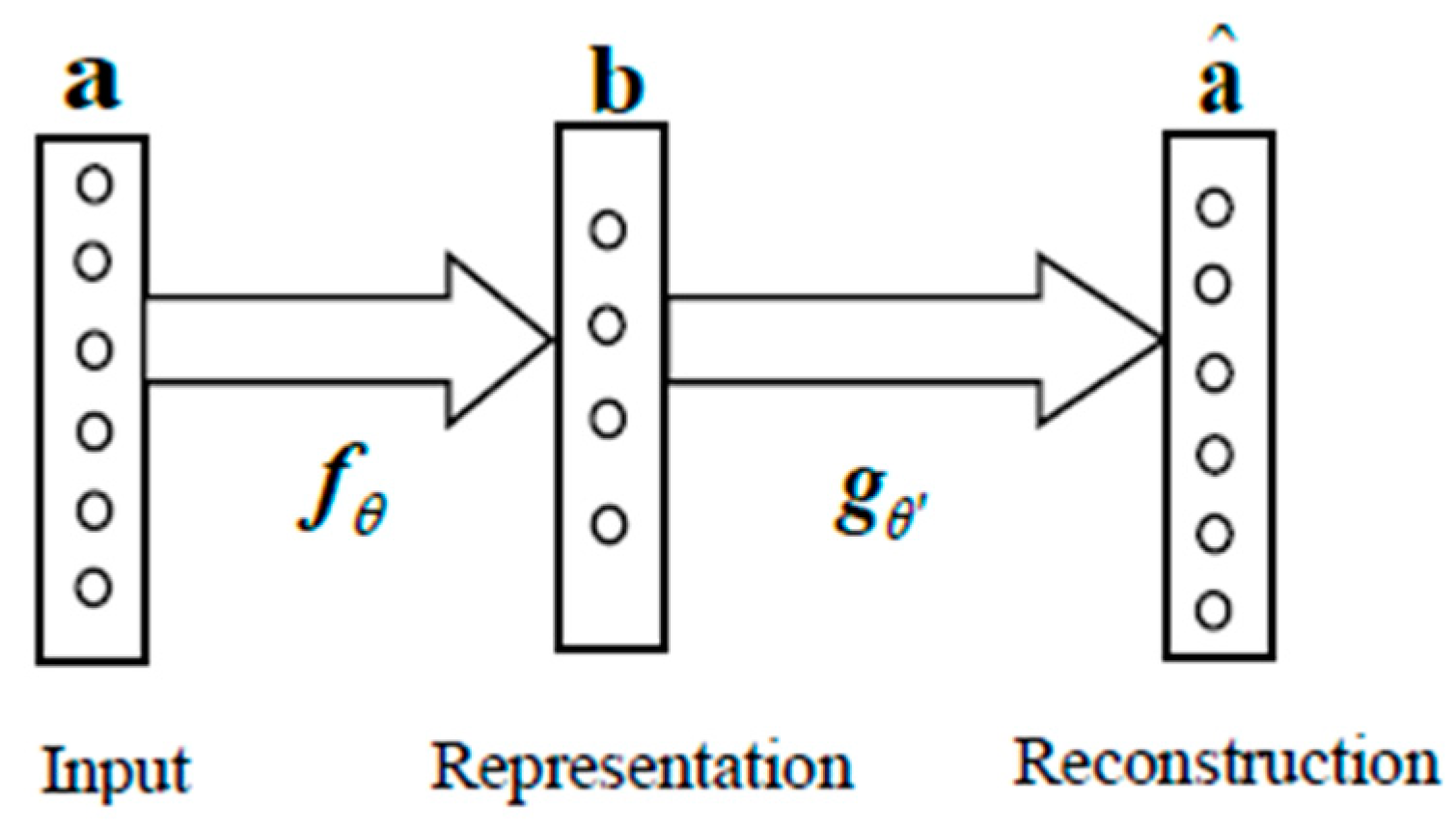
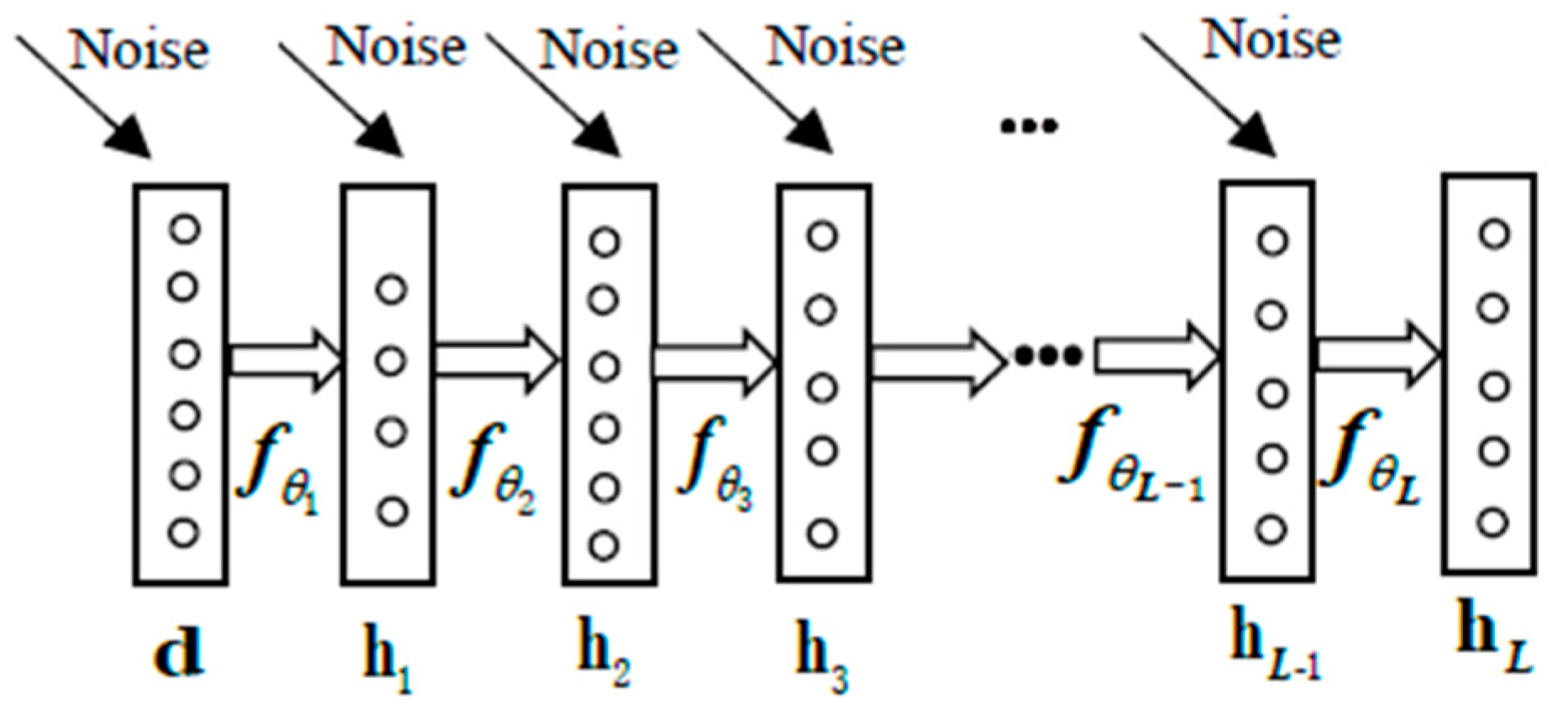
3.2. Feature Extraction by Stacked Denoising Autoencoders

3.2.1. AutoEncoder (AE)

First, we introduce the principle of traditional autoencoder (AE) [44,45], which is the base of denoising autoencoder (DAE) [33]. The typical structure of autoencoder (AE) can be illustrated by Figure 2.
As shown in Figure 2, a traditional autoencoder is a simple neural network with three layers containing an input layer, representation layer, and reconstruction layer. Different from the common neural network, the output of AE is the reconstruction of input data, with the training objective to minimize the reconstruction error.
Let a denote input vector of a data object, which can be encoded to a feature representation b by a nonlinear activation function f θ , as shown in (3).
b = f θ ( a )
Then, another nonlinear function g θ can be employed to decode the feature representation b to a vector a ^ , the reconstruction of the input vector a , as illustrated in (4).
a ^ = g θ ( b )
The parameters θ and θ are optimized according to the principle of minimizing the sum of reconstruction error of all data objects.

3.2.2. Stacked Denoising Autoencoders (SDAE)

A denoising autoencoder (DAE) [33], a simple variant of AE, was designed to acquire more robust representations by learning from a corrupted input with adding some noise into initial input, such as Gaussian noise, or some values being setting to zeros. Stacked denoising autoencoders (SDAE), has succeeded in a variety of application domains, such as the user response prediction based on encoded categorical attributes by one-hot technique [43] and acoustic object recognition [46]. Let d ˜ denote a corrupted version of an initial input vector d . Similar to AE, d ˜ can be encoded to a representation h by f θ , then the reconstruction vector d ^ of the uncorrupted input vector can be obtained from h by g θ .
Giving the initial values at random, the parameters θ and θ can be optimized with adaptive gradient algorithm (Adagrad) [47] by minimizing the sum of reconstruction error between reconstructed vector d ^ i and corresponding uncorrupted input vector d i over entire dataset, as shown in (5).
E = d i d ^ i 2 2 = d i g θ ( f θ ( d ˜ i ) ) 2 2
With optimized parameters θ , we can calculate the first feature representation h 1 of each input vector d by f θ .Then, by taking h 1 as the input of second DAE and discarding the reconstruction layer, the second feature representation h 2 can be acquired using optimized parameters. In this way, stacked denoising autoencoders (SDAE) can be constructed by stacking some DAEs, with taking the feature representation vector of previous DAE as the input vector of the next DAE and discarding the reconstruction layer of previous DAE after layer-wise training. In the SDAE, each feature representation layer is corresponding to a hidden layer of common neural network. A typical structure of SDAE can be illustrated as Figure 3.
By adding noise to the uncorrupted input vector d , the vector d is transformed into corrupted input d ˜ , which can be mapped into the first feature representation h 1 by training the first DAE. By taking h 1 as the uncorrupted input vector of the second DAE, the second feature representation h 2 can be acquired in a similar way. Similarly, feature representations h 3 , , h L can also be obtained, where L is the number of feature representation layers, i.e., the number of hidden layers. As Zhang et al. suggested in [43], the optimal number of hidden layers in SDAE can be set at three, which is also validated by our experiment. The feature representations extracted by SDAE will deteriorate when the number of hidden layers is too big or too small.
In the SDAE, besides the optimization layer by layer, the parameters θ i ( 1 i L ) can be fine-tuned simultaneously to minimize the sum of reconstruction error between the uncorrupted preprocessed data vectors and corresponding representation vectors in the L th representation layer using the back propagation algorithm [48], where L is the number of representation layers. In addition, dropout noise [49] is used to prevent our SDAE from overfitting. By reconstructing a repaired input from an input with noise, the feature representations extracted by SDAE become more robust to noise [33].

3.2.3. Feature Construction for Clustering

After layer-wise optimization and fine-tuning of SDAE mentioned above, the optimal values of parameter θ i ( 1 i L ) can be acquired. For each data object x i , we can calculate its corresponding representation vectors of L layers, h 1 i , h 2 i , , h L i , based on these optimal values of parameters θ i ( 1 i L ) .
As Shelhamer et al. illustrated in [50], we can concatenate the representation vectors of L layers and express the clustering features of data object i as f i in (6),
f i = ( h 1 i , h 2 i , , h L i )
where i = 1 , 2 , , N .
Consequently, the original mixed dataset X can be converted to a real feature matrix F , as shown in (7).
F = ( f 1 , f 2 , , f N ) T
After preprocessing and feature extraction, the original mixed data space are transformed into a real Euclidean space, in which traditional numerical clustering algorithms can be employed to cluster mixed data objects. In this paper, due to its effectivity and insensitivity to data distribution, the modified density peaks clustering (DPC) method was chosen to perform our clustering tasks.

3.3. Density Peak Clustering and Its Improvement

The core of density peaks clustering (DPC) [20] is the determination of the cluster centers, which are data objects with high density and large local distance from other data objects having higher density. For each data object, we firstly define the distance between two data objects so as to calculate the density and local distances from other data objects with higher density. Let f i and f j denote clustering features of data object x i and data object x j respectively, then distance d i j ( 1 i N , 1 j N ) can be defined by (8).
d i j = f i f j 2
Giving a neighborhood ratio t in DPC, the cutoff distance d c can be found from sorted distances of all object pairs. Then, we calculate the local density ρ i of data object x i ( 1 i N ) by (9).
ρ i = j i exp ( d i j 2 d c 2 )
The relative distance δ i of data object x i can be defined by (10).
δ i = { min j : ρ j > ρ i { d i j } , if   { j : ρ j > ρ i } ϕ max j { δ j } , otherwise
After calculating local densities and relative distances of all data objects, we can identify the cluster centers manually with the help of a decision graph in DPC [20], a scatter plot of local density vs. relative distance. Usually, the data objects with anomalously large local densities and relative distances are recognized as cluster centers, which always locate at the upper right hand corner of the decision graph. For some complex datasets, DPC can draw a γ graph of γ i ( = ρ i δ i ) (in descending order) vs. i to aid users to select cluster centers. However, this human-based selection of cluster centers is a tremendous barrier in intelligent analysis of data [51]. Thus, we present an automatic parameter-free selecting cluster centers to improve DPC.
In order to eliminate the effect of the local density and relative distance in different magnitudes, we normalize them by (11) and (12), respectively.
μ i = ρ i max 1 j N { ρ j }
ν i = δ i max 1 j N { δ j }
To facilitate determination of the cluster number automatically, we introduce γ i , which can be calculated by (13),
γ i = μ i ν i
Generally speaking, the larger the value of γ i is, the more likely the data object x i becomes a cluster center. Thus, we can sort all data objects by γ i in descending order and draw an evaluation graph of sorted γ i vs. i , then choose the first k data objects sorted in descending order according to γ as cluster centers, which k is determined by L-method [52,53] automatically.
The L-method is an approach to finding the knee point from a series of points by fitting two straight lines with the points on the left side of candidate knee and on the right side of it respectively according to the principle of minimizing the total root mean squared error. The intersection point of two straight lines fitted most closely can be viewed as the knee point, which can be used to determine the number of cluster centers. For data points with a long tail, the knee point found by L-method may be inconsistent with the true knee due to the serious imbalance on two sides of candidate knee point in the number of data points. To overcome this issue, a method for iterative refinement of the knee point [39] was proposed to adjust focus region iteratively so that L-method could find the true knee point in a few iterations.
To overcome the drawback of selecting the number of cluster centers by decision graph manually in DPC-based algorithms, we employed the L-method with iterative refinement to determine the cluster number automatically based on sorted γ values of all data objects. For example, iterative refinement of the knee point requires only 3 iterations to obtain the final cluster number on Credit dataset with 653 data points in our experiment, as shown in Figure 4, Figure 5 and Figure 6, respectively.
After determination of the cluster centers, each remaining data object can be assigned to a cluster, whose cluster center is nearest to the corresponding data object.

3.4. Algorithm Summarization and Time Complexity Analysis

The proposed DPC-SDAE algorithm can be summarized as the following Algorithm 1.
Algorithm 1. DPC-SDAE algorithm
Inputs:mixed dataset X consisting of N data objects, the initial value of encoding parameters θ and decoding parameters θ , and cutoff distance d c .
Outputs:cluster label vector c = [ c 1 , c 2 , , c N ] .
Steps: 1.Transform categorical attributes into a binary matrix Z by one-hot encoding.
2.Normalize numerical attributes by (2) and concatenate with the binary matrix Z to obtain a matrix D = ( d 1 , d 2 , , d N ) T .
3.Input D to SDAE with the initial value of θ and θ to extract clustering features and construct a normalized feature matrix F = ( f 1 , f 2 , , f N ) T .
4.Calculate distances between objects based on F by (8).
5.Calculate and normalize the local densities of data objects based on cutoff distance d c by (9) and (11).
6.Calculate and normalize the relative distances of data objects by (10) and (12).
7.Calculate γ by (13) and sort data objects by γ in descending order.
8.Determine the number of clusters k with L-method and select k data objects with larger γ as cluster centers.
9.Assign each remaining data object a cluster label as the same as its nearest cluster center.
10.Return the cluster label vector c = [ c 1 , c 2 , , c N ] .
The time complexity of our proposed DPC-SDAE algorithm is illustrated as follows. To keep consistency of notations with Algorithm 1, we let N denote the number of data objects, p is the number of categorical attributes, m p is the number of numerical attributes, s is the average number of distinct categorical attribute values, L is the number of hidden layers in SDAE, and N 0 , N 1 , N 2 , , N L represent the number of the neural units in input layer and L hidden layers, and I m a x denotes the maximum number of iterations for adaptive gradient algorithm in each layer. The cost of data preprocessing is O ( N ( p s + m p ) ) and extracting features by SDAE requires O ( N I m a x l = 1 L N l 1 N l ) . There are O ( N 2 ) to calculate distances between data objects, local densities, and relative distances of all data objects. The quick sorting of local densities needs O ( N log N ) and the cost of using L-method to determine the cluster number and assignment of remaining data objects to their clusters is O ( N ) . Therefore, the total time cost of our proposed DPC-SDAE algorithm in this paper is O ( N ( p s + m p ) ) + O ( N I m a x l = 1 L N l 1 N l ) + O ( N 2 ) + O ( N log N ) + O ( N ) . As it usually has p s + m p N , the overall time complexity of our DPC-SDAE algorithm can be viewed as O ( N I m a x l = 1 L N l 1 N l ) + O ( N 2 ) .

4. Results and Discussion

In this section, we show our experiments on some datasets from UCI machine learning repository [54] to validate our proposed DPC-SDAE algorithm by comparing with OCIL [13], k-prototypes [12], and DPC-M [22]. In addition, the evaluation indexes adopted and the impact of five hyperparameters on clustering quality are also introduced. All experiments were conducted on a laptop with Intel Core i5-5257U 2.7 GHz CPU and 8 GB RAM implementing MATLAB 2013a with Windows 8 operating system.

4.1. Datasets

To illustrate the extensive applications of our proposed method, the datasets in our experiments contain one pure numerical attribute dataset, one pure categorical dataset, and four mixed datasets, whose basic information are shown in Table 1.
Among six datasets, Iris is a pure numerical attribute dataset and Vote is a pure categorical attribute dataset, whereas the other four datasets are composed of mixed data with both categorical attributes and numerical attributes. Before performing experiments, the data objects containing missing values were removed from corresponding datasets, for example, eight data objects with missing values are eliminated from 366 data objects in Dermatology dataset. In Abalone dataset, nine data objects are deleted as outliers due to that they belong to the classes consisting of only one or two data objects. Adult_10,000 is a subset of Adult containing 10,000 data objects selected randomly after the removal of data objects containing missing values.

4.2. Evaluation Indexes

In order to evaluate the clustering quality, we introduced two evaluation indexes for clustering: clustering accuracy (ACC) [13,14,55] and the rand index (RI) [39,56]. These two indexes are used extensively to validate the clustering algorithms.
Let N stand for the number of data objects in the dataset, c = ( c 1 , c 2 , , c N ) denotes the cluster label vector acquired from the clustering algorithm, and b = ( b 1 , b 2 , , b N ) represents the ground truth label vector of all data objects. The ACC can be calculated by (14).
ACC = j = 1 N δ ( b j , map ( c j ) ) N
where map ( ) is the optimal mapping function obtained by Hungarian algorithm [57], which maps each cluster label into a ground truth label, and δ ( x , y ) is the Kronecker delta function, whose value equals 1 if x = y and 0 otherwise. In general, the larger the value of ACC is, the higher the clustering quality.
The second index to measure the clustering quality is rand index (RI) based on the relations between pairwise data objects from two partitions of the same dataset. Let P and Q be the ground truth partition and a clustering partition of a dataset with N data objects, respectively. Let a 1 denote the number of pairs of data objects that belong to the same class in P and the same cluster in Q , a 2 stands for the number of pairs of data objects that are placed in the different classes in P and the different clusters in Q , a 3 denotes the number of pairs of data objects that are in the same class in P and belong to the different clusters in Q , and a 4 represents the number of pairs of data objects that belong to the different classes in P and are in the same cluster in Q . RI can be calculated by (15).
RI = a 1 + a 2 j = 1 N a j
Similar to ACC, the larger the RI is, the better the clustering result.

4.3. Clustering Results and Analysis

In the experiments, the clustering performance of our proposed DPC-SDAE clustering algorithm is compared with k-prototypes [12], OCIL [13], and DPC-M [22] algorithms on six different datasets. Among them, k-prototypes is the most classical clustering algorithm for mixed data, and OCIL is an efficient partition-based clustering algorithm being free of certain parameters, while DPC-M proposed in 2017 is an algorithm based on DPC for clustering mixed data by defining a united distance for categorical and numerical attributes. With the exception of the DPC-M algorithm, the clustering performance of the remaining three algorithms was affected by the initial cluster prototypes or initial parameters selected randomly. To eliminate the impact of random initialization, we executed each algorithm thirty times on each dataset and investigated them statistically except DPC-M, i.e., took into account the mean and standard deviation of evaluation index values. In k-prototypes and OCIL, the cluster number k was set at the number of actual classes. The adjustment parameter γ in k-prototypes was set at a half of the average standard deviation of numerical attribute values, as the same as in [13]. The k-means was conducted on pure numerical attribute Iris dataset instead of k-prototypes, whereas k-prototypes was replaced by k-modes on pure categorical attribute Vote dataset. In DPC-M algorithm, the cutoff distance d c was calculated based on the neighborhood ratio t being 1.5% [22].
In our proposed DPC-SDAE algorithm, the structure of SDAE and hyperparameters are set as identically as possible on all datasets in our experiments. Specifically, three denoising autoencoders with the same number of hidden neural units were stacked to constitute SDAE to extract clustering features of each dataset. As each denoising autoencoder contains only one hidden layer, the number of hidden layers adopted in our DPC-SDAE algorithm is three unless otherwise stated. The sigmoid function was adopted as encoding and decoding functions, whose parameters was optimized by adaptive gradient algorithm (Adagrad) [47]. The important hyperparameters in DPC-SDAE algorithm were set as follows. The neighborhood ratio in DPC, the epsilon in Adagrad and the number of optimization epochs were set respectively at 4%, 10−8, and 100 on all datasets. The dropout ratio, the learning rate, and the number of neural units in the hidden layer were set at 0.2, 0.1, and the same as the size of input data on four small sample datasets, respectively. On Abalone and Adult_10000, the dropout ratio and the learning rate were set at 0.1 and 0.03, respectively. The number of neural units in hidden layer on these two datasets were set at 10 and 55, respectively.
Table 2 and Table 3 provide the main results of our experiments. The values of ACC and RI corresponding to the algorithm with the best performance are accentuated in bold for each dataset.
As shown in Table 2, it is obvious that our proposed DPC-SDAE algorithm is much superior to other three clustering algorithms on five datasets in terms of ACC from the viewpoint of statistics. It can be observed that our proposed DPC-SDAE algorithm acquires a larger mean of ACC values than three benchmark algorithms on six datasets. For instance, the mean of ACC was improved by 21.7%, 12.6%, and 12.3% on the Dermatology dataset compared with k-prototypes, OCIL, and DPC-M, respectively. In addition, the standard deviation of ACC generated by the DPC-SDAE algorithm is much smaller on most of datasets, which means that the DPC-SDAE algorithm is more robust.
It can be observed from Table 3 that our proposed DPC-SDAE algorithm statistically performs better than the other three baseline clustering algorithms on six datasets in terms of IR. It can be seen that DPC-SDAE algorithm obtains much larger mean of IR values than three baseline algorithms on six datasets. In addition, the standard deviation of IR generated by DPC-SDAE algorithm is much smaller than that resulted from k-prototypes and OCIL on most of datasets, which signifies that DPC-SDAE algorithm has greater robustness. It is noteworthy that DPC-SDAE algorithm increases the IR onsix datasets. For instance, the mean of IR is improved by 11.2%, 7.7%, and 6.8% on the Dermatology dataset compared with k-prototypes, OCIL, and DPC-M, respectively.
The main reason for the higher clustering quality and more robust results achieved by our proposed DPC-SDAE algorithm is that the feature representations extracted by SDAE are more robust and discriminating than original data attributes. Moreover, the subsequent DPC algorithm adopted by DPC-SDAE can further improve clustering performance, especially on datasets with nonspherical distribution.

4.4. Discussion on Hyperparameters in DPC-SDAE Algorithm

In this part, we discuss the relations between clustering quality and five hyperparameters in DPC-SDAE algorithm, performing on the Credit dataset as an example. In our experiment, we vary only one hyperparameter by fixing other hyperparameters every time.

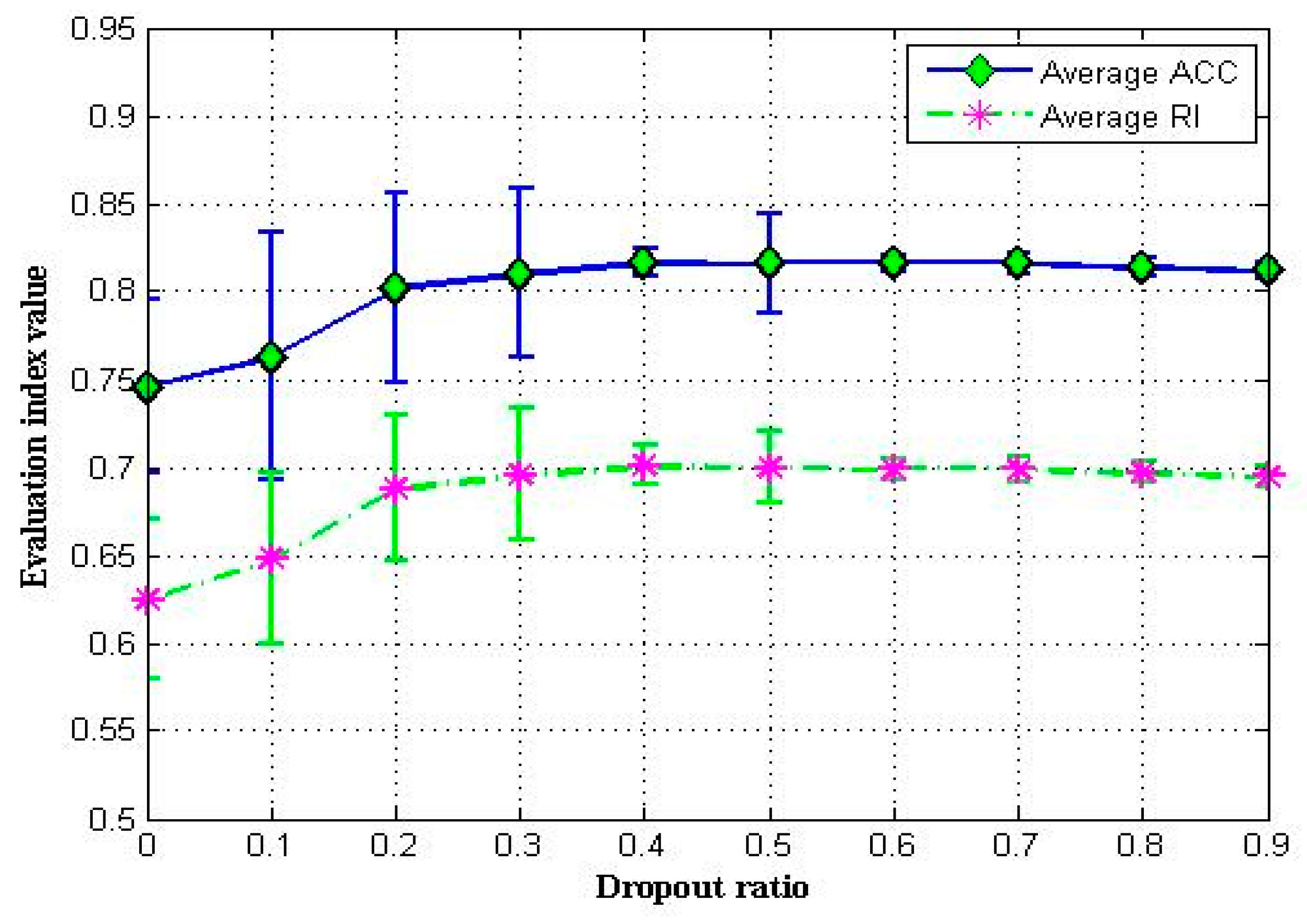
4.4.1. Dropout Ratio

Dropout is a technique to address overfitting of stacked denoising autoencoders by randomly dropping units (along with their connections) from the deep neural network during training [49]. As an important index for describing the degree of dropout, the dropout ratio plays a key role in the DPC-SDAE algorithm.
We varied the dropout ratio from 0 to 0.9 with an increment of 0.1 on the condition that the learning rate, the number of neural units in each hidden layer, and the neighbor ratio were set at 0.1, 46, and 4%, respectively. As shown in Figure 7, we can observed that both average ACC and RI firstly go up significantly with the increasing of dropout ratio when dropout ratio is less than 0.3, then reach the maximum value point when the dropout ratio is at 0.4. Both the average ACC and RI deteriorated slightly when the dropout ratio was greater than 0.4. Thus, 0.4 can be viewed as the optimal dropout ratio on the Credit dataset.

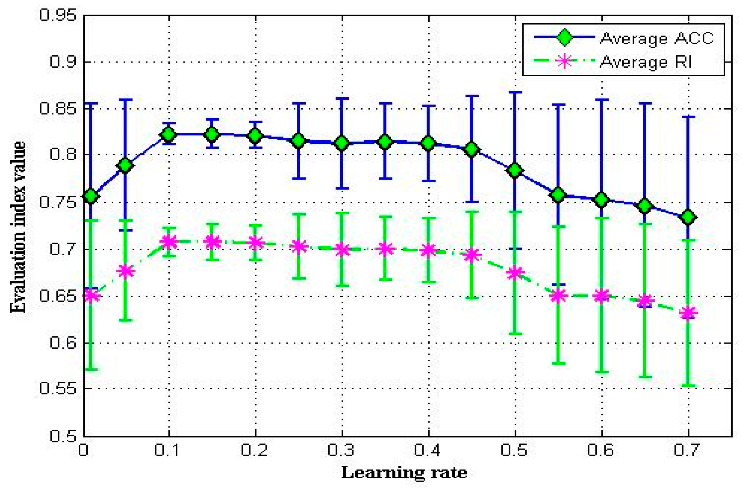
4.4.2. Learning Rate

The learning rate is a hyperparameter to affect the speed of weights updating in optimization of encoding and decoding functions in SDAE. To investigate the impact of learning rate, we fixed the dropout ratio, the number of neural units in each hidden layer, and the neighbor ratio at 0.2, 46, and 4%, respectively. We investigated the relationship between evaluation indexes of DPC-SDAE algorithm and the learning rate.
From Figure 8, it can be obviously seen that the average ACC and RI improve dramatically when the learning rate is less than 0.1. When the learning rate lies between 0.1 and 0.4, average ACC and RI are almost unchanged. If we continued to increase the learning rate, both the average ACC and RI would go down significantly and have larger standard deviations when the learning rate is greater than 0.4. Taking into account the larger average value and the lower deviations in terms of ACC and RI, the optimal learning rate can be set at 0.1 on the Credit dataset.

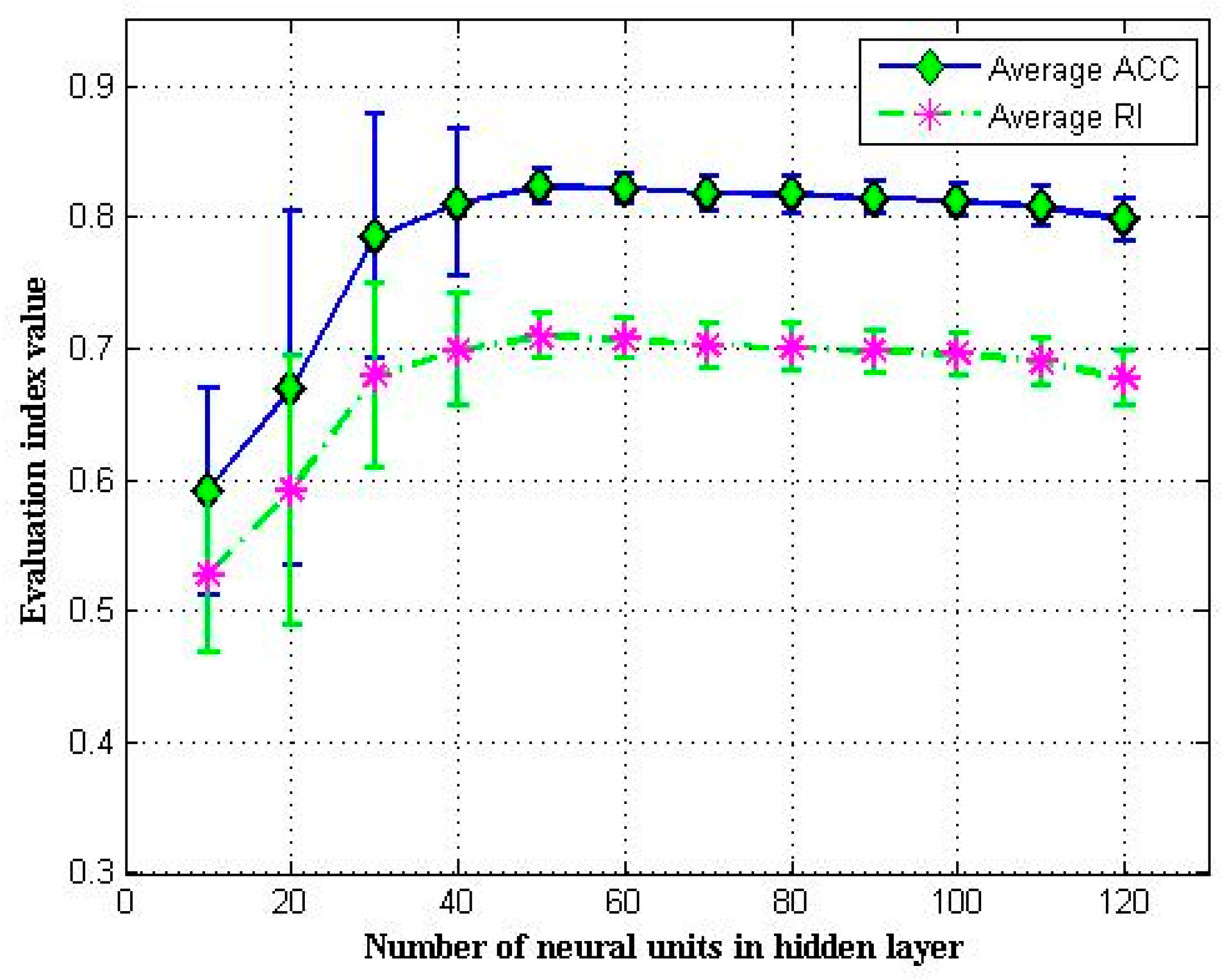
4.4.3. Number of Neural Units in Hidden Layer

The hidden layer architecture is an important factor for extracting useful clustering features. According to the suggestion from [43], the SDAE consisting of three hidden layers with equal number of neural units was employed in our experiment. Thus, we need only take into account the impact of the number of neural units in hidden layer. Fixing the dropout ratio, the learning rate, and the neighbor ratio at 0.2, 0.1, and 4%, respectively, we can observe how ACC and RI change with different numbers of neural units in the hidden layer.
As illustrated in Figure 9, both average ACC and RI rise significantly with the increasing of the number of neural units in hidden layer at first, then change little when the number of neural units in hidden layer is greater than about 50. Thus, choosing 50 as the optimal number of neural units in hidden layer is appropriate on Credit dataset by jointly considering about evaluation indexes and computational complexity.

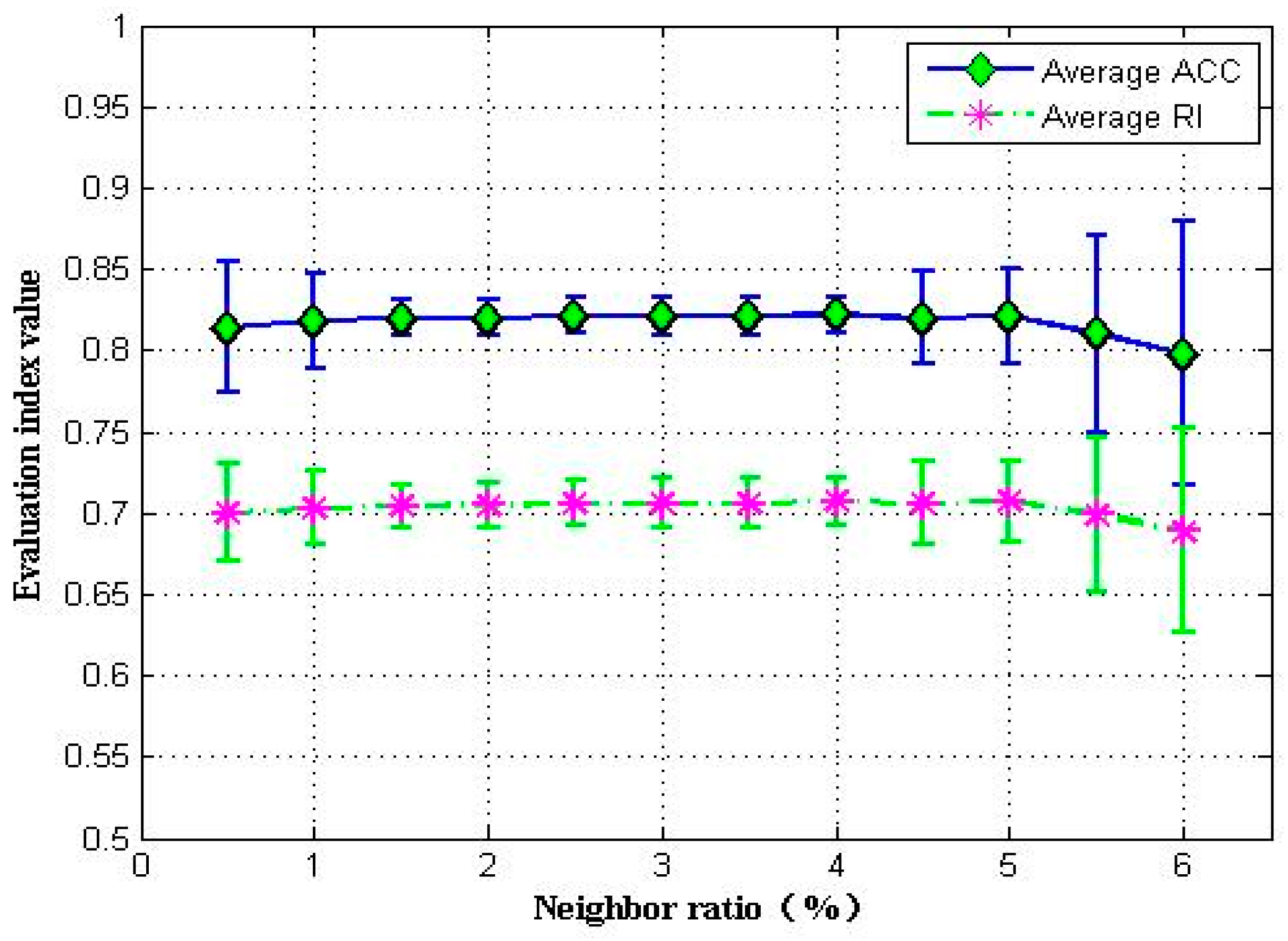
4.4.4. Neighbor Ratio

The cutoff distance—the important parameter in DPC-SDAE determined by the neighbor ratio—significantly affects the clustering quality. As before, we fixed the dropout ratio, the learning rate, and the number of neural units in each hidden layer at 0.2, 0.1, and 46, respectively.
By varying the percent of neighbors from 0.5% to 6% with an increment 0.5%, we can observe from Figure 10 that both the average ACC and RI change little when the neighbor ratio is less than 5% whereas they go down sharply with large deviation when the neighbor ratio is greater than 5%. Taking into account the larger average value and the lower deviations in terms of ACC and RI, the optimal neighbor ratio can be set at 4% on Credit dataset.

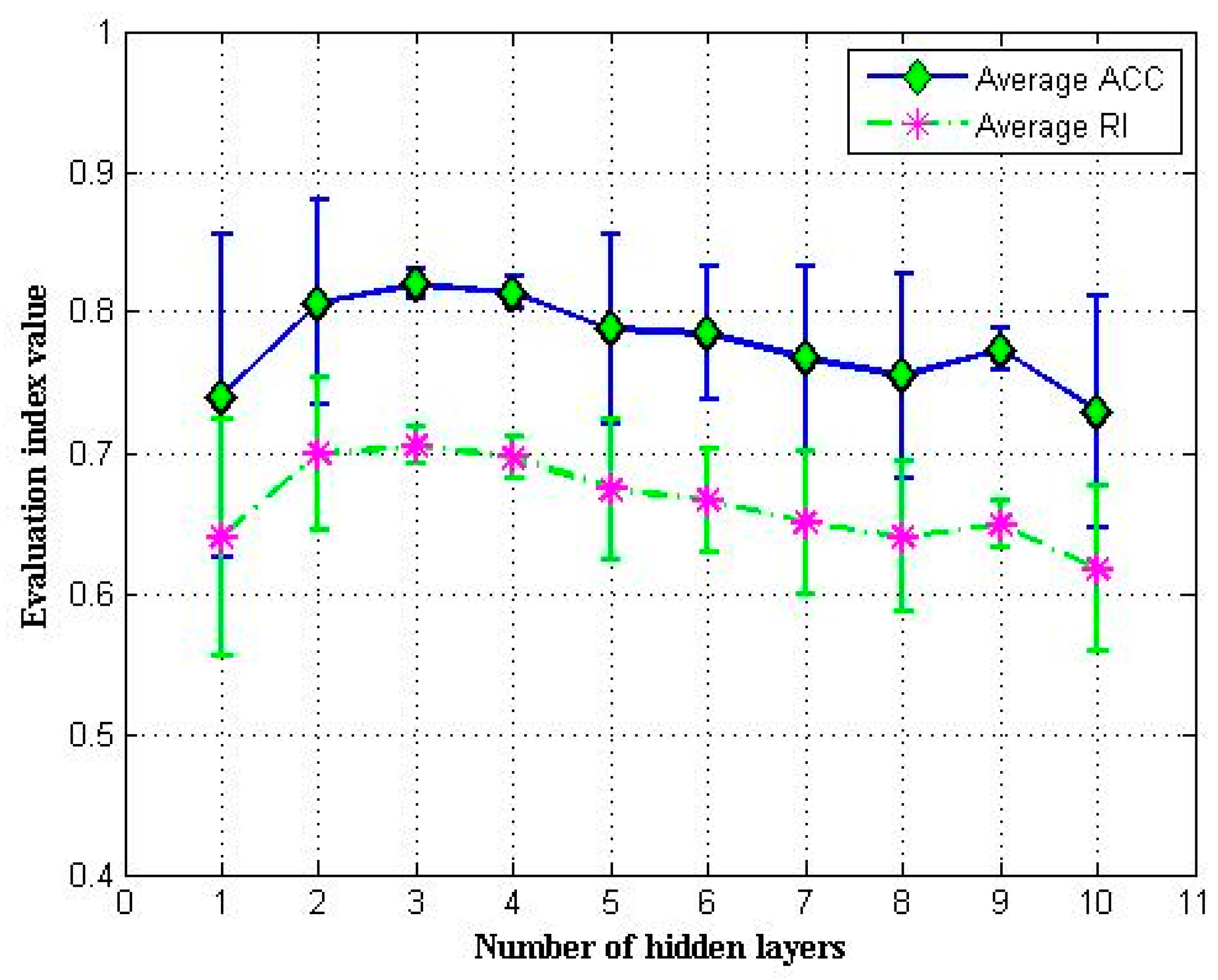
4.4.5. Number of Hidden Layers

The number of hidden layers also plays an important role in our DPC-SDAE algorithm. To investigate the impact of the number of hidden layers, we fixed the learning rate, the dropout ratio, the number of neural units in each hidden layer, and the neighbor ratio at 0.1, 0.2, 46, and 4%, respectively. We investigated the relationship between evaluation indexes of DPC-SDAE algorithm and the number of hidden layers.
As shown in Figure 11, with the number of hidden layers being changed from 1 to 10 with an increment 1, both average ACC and RI increase at first and then deteriorate slowly when the number of hidden layers is greater than three. Thus, the optimal number of hidden layers can be set at three on Credit dataset.

4.5. Discussion on the Generalization of the Results

Our proposed DPC-SDAE framework applies to not only clustering objects with mixed attributes, but also to clustering pure categorical attribute objects or pure numerical attribute objects. The SDAE in the framework can be generalized to other common deep learning structures, such as variational autoencoder (VAE), generative adversarial network (GAN). In our experiments, the data objects with missing attribute values are deleted directly before employing DPC-SDAE. In data preprocessing stage, we can fill in missing attribute values by utilizing imputation methods of missing values. For example, we can use the mean value of each numerical attribute on entire dataset to replace the corresponding missing values or take the mode value of each categorical attribute on entire dataset as the imputation values of corresponding missing categorical attribute values. Thus, our DPC-SDAE framework can be generalized to perform clustering mixed data with missing attribute values.

4.6. Discussion on the Methodological and Practical Implications

Our proposed DPC-SDAE algorithm provides an effective method for clustering mixed data, it improves the traditional density peaks clustering, which extends its clustering objects from numerical attribute data to mixed data with both numerical attributes and categorical attributes. L-method with iterative refinement of the knee point can also be applied to determining the number of clusters automatically for other clustering methods for mixed data by replacing the sorted γ values with corresponding clustering quality index of all data objects.
Our proposed DPC-SDAE algorithm also makes better decisions in practical problems. For example, by clustering credit card applicants in Credit dataset with DPC-SDAE algorithm, bank credit officer can obtain two clusters and corresponding cluster centers, which represent the prototypes of approval applicants and denial applicants, respectively. When the attribute values of a new credit card applicant are submitted, the distances between this credit card applicant and each cluster center can be calculated. Consequently, a bank credit officer can decide to approve or reject the credit card application by the principle of the nearest neighbor. In clinical medicine, patients with heart disease can also be recognized from healthy persons by employing DPC-SDAE algorithm.

4.7. Discussion on the Limitations of DPC-SDAE

In our proposed DPC-SDAE algorithm, the improved density peaks clustering is employed to conduct clustering on mixed data objects based on the feature representations extracted by SDAE. The cutoff distance, or corresponding neighbor ratio, plays an important role in clustering mixed data, but it is usually prespecified manually and incapable of determining automatically on each dataset. In the future research, we will investigate the methods for adaptively determining the cutoff distance or neighbor ratio on different datasets.

5. Conclusions

In this paper, we have proposed a clustering algorithm named DPC-SDAE, which integrates stacked denoising autoencoders and density peaks clustering algorithm to perform clustering for various data types. Based on the robust clustering features learned from SDAE instead of the original attributes, the DPC-SDAE algorithm can acquire more accurate and robust clustering results, which have been experimentally validated in comparison with three baseline algorithms. In addition, density peaks clustering algorithm has been improved by employing L-method to determine the number of cluster centers automatically, which overcomes the drawback of selecting the number of cluster centers by decision graph manually in original DPC algorithm. We also experimentally investigated the effect of some hyperparameters on clustering quality in DPC-SDAE. We found that each hyperparameter has a relatively large range of values, in which the evaluation indexes of DPC-SDAE keep almost unchanged. This is vitally important since it is unfeasible to optimize hyperparameters by cross validation method in most of clustering tasks due to the lack of ground truth labels of data objects. Our experiment results have also demonstrated that stacked denoising autoencoders can be applied to clustering small sample data effectively besides extensive applications in clustering large scale data.
In the future, we aim to investigate the integration of DPC algorithm and deep generative model, such as variational autoencoder (VAE), generative adversarial network (GAN), to improve the clustering quality even more. Future research will also include the methods for adaptively determining cutoff distance in DPC.

Author Contributions

Conceptualization, B.D. and Z.G.; Methodology, B.D. and L.H.; Formal Analysis, B.D. and Y.Y.; Resources, B.D.; Data Curation, B.D.; Writing—Original Draft Preparation, B.D.; Writing—Review and Editing, L.H. and Z.G.; Visualization, S.C.; Supervision, L.H.; Project Administration, B.D. and L.H.; Funding Acquisition, B.D.

Funding

This work was partially supported by the Key Natural Science Foundation of the Colleges and Universities in Anhui Province of China under Grant No. KJ2016A592, KJ2017A547, and KJ2018A0564, the Outstanding Youth Talent Foundation of Hefei University under Grant No. 16YQ11RC, the Fostering Master’s Degree Empowerment Point Project of Hefei University under grant No. 2018xs03, the Postgraduate Research&Practice Innovation Program of Jiangsu Province of China under Grant No. KYCX17_0486, the Fundamental Research Funds for the Central Universities under Grant No. 2017B708X14, the Research Project of Human Resources and Social Security in Hebei Province of China under Grant No. JRSHZ-2018-08018, the Natural Science Foundation of the Colleges and Universities in Anhui Province of China under Grant No. KJ2017B016, the Jiangsu Provincial Key Constructive Laboratory for Big Data of Psychology and Cognitive Science under Grant No. PDLAB201807, and the Natural Science Project of the Higher Education Institutions of Jiangsu Province of China under Grant No. 18KJD520005.

Acknowledgments

The authors thank Kyunghyun Cho for sharing his deepmat toolbox that provided convenience for this work, and also thank the reviewers and editors for giving us constructive suggestions which help us to improve the quality of this paper.

Conflicts of Interest

The authors declare no conflicts of interest.

References

  1. Ushakov, A.; Klimentova, X.; Vasilyev, I. Bi-level and Bi-objective p-Median Type Problems for Integrative Clustering: Application to Analysis of Cancer Gene-Expression and Drug-Response Data. IEEE/ACM Trans. Comput. Biol. Bioinform. 2018, 15, 46–59. [Google Scholar] [CrossRef] [PubMed]
  2. Wang, Q.; Chen, G. Fuzzy soft subspace clustering method for gene co-expression network analysis. Int. J. Mach. Learn. Cybern. 2017, 8, 1157–1165. [Google Scholar] [CrossRef]
  3. Subudhi, S.; Panigrahi, S. A hybrid mobile call fraud detection model using optimized fuzzy C-means clustering and group method of data handling-based network. Vietnam J. Comput. Sci. 2018, 5, 205–217. [Google Scholar] [CrossRef]
  4. Han, C.Y. Improved SLIC imagine segmentation algorithm based on K-means. Clust. Comput. 2017, 20, 1017–1023. [Google Scholar] [CrossRef]
  5. Ahmadi, P.; Gholampour, I.; Tabandeh, M. Cluster-based sparse topical coding for topic mining and document clustering. Adv. Data Anal. Classif. 2018, 12, 537–558. [Google Scholar] [CrossRef]
  6. Sutanto, T.; Nayak, R. Fine-grained document clustering via ranking and its application to social media analytics. Soc. Netw. Anal. Min. 2018, 8, 1–19. [Google Scholar] [CrossRef]
  7. MacQueen, J. Some methods for classification and analysis of multivariate observations. In Proceedings of the Fifth Berkeley Symposium on Mathematical Statistics and Probability, Berkeley, CA, USA, 21 June–18 July 1965; Volume 1, pp. 281–297. [Google Scholar]
  8. Ester, M.; Kriegel, H.P.; Xu, X. A density-based algorithm for discovering clusters in large spatial databases with noise. In Proceedings of the Second International Conference on Knowledge Discovery and Data Mining(KDD’96), Portland, OR, USA, 2–4 August 1996; pp. 226–231. [Google Scholar]
  9. Donath, W.E.; Hoffman, A.J. Lower Bounds for the Partitioning of Graphs. IBM J. Res. Dev. 1973, 17, 420–425. [Google Scholar] [CrossRef]
  10. Wang, Y.; Duan, X.; Liu, X.; Wang, C.; Li, Z. A spectral clustering method with semantic interpretation based on axiomatic fuzzy set theory. Appl. Soft Comput. 2018, 64, 59–74. [Google Scholar] [CrossRef]
  11. Bianchi, G.; Bruni, R.; Reale, A.; Sforzi, F. A min-cut approach to functional regionalization, with a case study of the Italian local labour market areas. Optim. Lett. 2016, 10, 955–973. [Google Scholar] [CrossRef]
  12. Huang, Z. Clustering Large Data Sets with Mixed Numeric and Categorical Values. In Proceedings of the Pacific-Asia Conference on Knowledge Discovery and Data Mining (PAKDD’97), Singapore, 22–23 February 1997; pp. 21–34. [Google Scholar]
  13. Cheung, Y.M.; Jia, H. Categorical-and-numerical-attribute data clustering based on a unified similarity metric without knowing cluster number. Pattern Recognit. 2013, 46, 2228–2238. [Google Scholar] [CrossRef]
  14. Ding, S.; Du, M.; Sun, T.; Xu, X.; Xue, Y. An entropy-based density peaks clustering algorithm for mixed type data employing fuzzy neighborhood. Knowl. Based Syst. 2017, 133, 294–313. [Google Scholar] [CrossRef]
  15. Ralambondrainy, H. A conceptual version of the K-means algorithm. Pattern Recognit. Lett. 1995, 16, 1147–1157. [Google Scholar] [CrossRef]
  16. He, Z.; Xu, X.; Deng, S. Scalable algorithms for clustering large datasets with mixed type attributes. Int. J. Intell. Syst. 2010, 20, 1077–1089. [Google Scholar] [CrossRef]
  17. Huang, Z. A Fast Clustering Algorithm to Cluster Very Large Categorical Data Sets in Data Mining. In Proceedings of the the SIGMOD Workshop on Research Issues on Data Mining and Knowledge Discovery (DMKD’97), Tucson, AZ, USA, 11 May 1997. [Google Scholar]
  18. Ji, J.; Pang, W.; Zhou, C.; Han, X.; Wang, Z. A fuzzy k-prototype clustering algorithm for mixed numeric and categorical data. Knowl. Based Syst. 2012, 30, 129–135. [Google Scholar] [CrossRef]
  19. Chatzis, S.P. A fuzzy c-means-type algorithm for clustering of data with mixed numeric and categorical attributes employing a probabilistic dissimilarity functional. Exp. Syst. Appl. 2011, 38, 8684–8689. [Google Scholar] [CrossRef]
  20. Rodriguez, A.; Laio, A. Clustering by fast search and find of density peaks. Science 2014, 344, 1492–1496. [Google Scholar] [CrossRef] [PubMed]
  21. Du, M.; Ding, S.; Xue, Y. A novel density peaks clustering algorithm for mixed data. Pattern Recognit. Lett. 2017, 97, 46–53. [Google Scholar] [CrossRef]
  22. Liu, S.; Zhou, B.; Huang, D.; Shen, L. Clustering Mixed Data by Fast Search and Find of Density Peaks. Math. Probl. Eng. 2017, 2017, 5060842. [Google Scholar] [CrossRef]
  23. Xie, J.; Girshick, R.; Farhadi, A. Unsupervised Deep Embedding for Clustering Analysis. In Proceedings of the 33nd International Conference on Machine Learning (ICML 2016), New York, NY, USA, 19–24 June 2016; pp. 478–487. [Google Scholar]
  24. Li, F.; Qiao, H.; Zhang, B. Discriminatively boosted image clustering with fully convolutional auto-encoders. Pattern Recognit. 2018, 83, 161–173. [Google Scholar] [CrossRef]
  25. Chen, G. Deep Learning with Nonparametric Clustering. Available online: http://arxiv.org/abs/1501.03084 (accessed on 13 January 2015).
  26. Hsu, C.C.; Huang, Y.P. Incremental clustering of mixed data based on distance hierarchy. Expert Syst. Appl. 2008, 35, 1177–1185. [Google Scholar] [CrossRef]
  27. Zhang, K.; Wang, Q.; Chen, Z.; Marsic, I.; Kumar, V.; Jiang, G.; Zhang, J. From Categorical to Numerical: Multiple Transitive Distance Learning and Embedding. In Proceedings of the 2015 SIAM International Conference on Data Mining (SIAM 2015), Vancouver, BC, Canada, 30 April–2 May 2015; pp. 46–54. [Google Scholar]
  28. David, G.; Averbuch, A. SpectralCAT: Categorical spectral clustering of numerical and nominal data. Pattern Recognit. 2012, 45, 416–433. [Google Scholar] [CrossRef]
  29. Jia, H.; Cheung, Y.M. Subspace Clustering of Categorical and Numerical Data with an Unknown Number of Clusters. IEEE Trans. Neural. Netw. Learn. Syst. 2018, 29, 3308–3325. [Google Scholar] [PubMed]
  30. Zheng, Z.; Gong, M.; Ma, J.; Jiao, L.; Wu, Q. Unsupervised evolutionary clustering algorithm for mixed type data. In Proceedings of the IEEE Congress on Evolutionary Computation (CEC 2010), Barcelona, Spain, 18–23 July 2010; pp. 1–8. [Google Scholar]
  31. Liu, X.; Yang, Q.; He, L. A novel DBSCAN with entropy and probability for mixed data. Clust. Comput. 2017, 20, 1313. [Google Scholar] [CrossRef]
  32. Behzadi, S.; Ibrahim, M.A.; Plant, C. Parameter Free Mixed-Type Density-Based Clustering. In Proceedings of the 29th International Conference Database and Expert Systems Applications (DEXA 2018), Regensburg, Germany, 3–6 September 2018; pp. 19–34. [Google Scholar]
  33. Vincent, P.; Larochelle, H.; Lajoie, I.; Bengio, Y.; Manzagol, P.A. Stacked Denoising Autoencoders: Learning Useful Representations in a Deep Network with a Local Denoising Criterion. J. Mach. Learn. Res. 2010, 11, 3371–3408. [Google Scholar]
  34. Hsu, C.; Lin, C. CNN-Based Joint Clustering and Representation Learning with Feature Drift Compensation for Large-Scale Image Data. IEEE Trans. Multimed. 2018, 20, 421–429. [Google Scholar] [CrossRef]
  35. Kingma, D.P.; Welling, M. Auto-Encoding Variational Bayes. Available online: http://arxiv.org/abs/1312.6114 (accessed on 1 May 2014).
  36. Goodfellow, I.; Pouget-Abadie, J.; Mirza, M.; Xu, B.; Warde-Farley, D.; Ozair, S.; Courville, A.; Bengio, Y. Generative Adversarial Nets. In Proceedings of the Advances in Neural Information Processing Systems 27 (NIPS’14), Montreal, QC, Canada, 8–13 December 2014; pp. 2672–2680. [Google Scholar]
  37. Jiang, Z.; Zheng, Y.; Tan, H.; Tang, B.; Zhou, H. Variational Deep Embedding: An Unsupervised and Generative Approach to Clustering. In Proceedings of the Twenty-Sixth International Joint Conference on Artificial Intelligence (IJCAI 2017), Melbourne, Australia, 19–25 August 2017; pp. 1965–1972. [Google Scholar]
  38. Chen, X.; Duan, Y.; Houthooft, R.; Schulman, J.; Sutskever, I.; Abbeel, P. InfoGAN: Interpretable Representation Learning by Information Maximizing Generative Adversarial Nets. In Proceedings of the Advances in Neural Information Processing Systems 29 (NIPS’16), Barcelona, Spain, 5–10 December 2016; pp. 2172–2180. [Google Scholar]
  39. Lam, D.; Wei, M.Z.; Wunsch, D. Clustering Data of Mixed Categorical and Numerical Type with Unsupervised Feature Learning. IEEE Access 2015, 3, 1605–1613. [Google Scholar] [CrossRef]
  40. Bu, F. A High-Order Clustering Algorithm Based on Dropout Deep Learning for Heterogeneous Data in Cyber-Physical-Social Systems. IEEE Access 2018, 6, 11687–11693. [Google Scholar] [CrossRef]
  41. Aljalbout, E.; Golkov, V.; Siddiqui, Y.; Cremers, D. Clustering with Deep Learning: Taxonomy and New Methods. Available online: http://arxiv.org/abs/1801.07648 (accessed on 13 September 2018).
  42. Min, E.; Guo, X.; Liu, Q.; Zhang, G.; Cui, J.; Long, J. A Survey of Clustering with Deep Learning: From the Perspective of Network Architecture. IEEE Access 2018, 6, 39501–39514. [Google Scholar] [CrossRef]
  43. Zhang, W.; Du, T.; Wang, J. Deep Learning over Multi-field Categorical Data: A Case Study on User Response Prediction. In Proceedings of the European Conference on Information Retrieval (ECIR 2016), Padua, Italy, 20–23 March 2016; pp. 45–57. [Google Scholar]
  44. Bengio, Y.; Lamblin, P.; Dan, P.; Larochelle, H. Greedy layer-wise training of deep networks. In Proceedings of the Advances in Neural Information Processing Systems 19 (NIPS’06), Vancouver, BC, Canada, 4–7 December 2006; pp. 153–160. [Google Scholar]
  45. Ranzato, M.A.; Poultney, C.S.; Chopra, S.; LeCun, Y. Efficient Learning of Sparse Representations with an Energy-Based Model. In Proceedings of the Advances in Neural Information Processing Systems 19 (NIPS’06), Vancouver, BC, Canada, 4–7 December 2006; pp. 1137–1144. [Google Scholar]
  46. Luo, S.; Zhu, L.; Althoefer, K.; Liu, H. Knock-Knock: Acoustic object recognition by using stacked denoising autoencoders. Neurocomputing 2017, 267, 18–24. [Google Scholar] [CrossRef]
  47. Duchi, J.; Hazan, E.; Singer, Y. Adaptive Subgradient Methods for Online Learning and Stochastic Optimization. J. Mach. Learn. Res. 2011, 12, 257–269. [Google Scholar]
  48. Rumelhart, E.D.; Hinton, E.G.; Williams, J.R. Learning representations by back-propagating errors. Nature 1986, 323, 533–536. [Google Scholar] [CrossRef]
  49. Srivastava, N.; Hinton, G.; Krizhevsky, A.; Sutskever, I.; Salakhutdinov, R. Dropout: A Simple Way to Prevent Neural Networks from Overfitting. J. Mach. Learn. Res. 2014, 15, 1929–1958. [Google Scholar]
  50. Shelhamer, E.; Long, J.; Darrell, T. Fully Convolutional Networks for Semantic Segmentation. IEEE Trans. Pattern Anal. Mach. Intell. 2017, 39, 640–651. [Google Scholar] [CrossRef] [PubMed]
  51. Bie, R.; Mehmood, R.; Ruan, S.S.; Sun, Y.C.; Dawood, H. Adaptive fuzzy clustering by fast search and find of density peaks. Personal Ubiquitous Comput. 2016, 20, 785–793. [Google Scholar] [CrossRef]
  52. Salvador, S.; Chan, P. Determining the number of clusters/segments in hierarchical clustering/segmentation algorithms. In Proceedings of the 2004 IEEE 16th International Conference on Tools with Artificial Intelligence (ICTAI 2004), Boca Raton, FL, USA, 15–17 November 2004; pp. 576–584. [Google Scholar]
  53. Zagouras, A.; Inman, R.H.; Coimbra, C.F.M. On the determination of coherent solar microclimates for utility planning and operations. Sol. Energy 2014, 102, 173–188. [Google Scholar] [CrossRef]
  54. Dua, D.; Taniskidou, E.K. UCI Machine Learning Repository. Available online: http://archive.ics.uci.edu/ml (accessed on 5 January 2019).
  55. Qian, Y.; Li, F.; Liang, J.; Liu, B.; Dang, C. Space Structure and Clustering of Categorical Data. IEEE Trans. Neural Netw. Learn. Syst. 2017, 27, 2047–2059. [Google Scholar] [CrossRef]
  56. Rand, W.M. Objective Criteria for the Evaluation of Clustering Methods. J. Am. Stat. Assoc. 1971, 66, 846–850. [Google Scholar] [CrossRef]
  57. Kuhn, H.W. The Hungarian method for the assignment problem. Nav. Res. Logist. 1955, 2, 83–97. [Google Scholar] [CrossRef]
Figure 1. The DPC-SDAE clustering framework.
Symmetry 11 00163 g001
Figure 2. Autoencoder (AE) structure.
Symmetry 11 00163 g002
Figure 3. Stacked denoising autoencoder (SDAE) structure.
Symmetry 11 00163 g003
Figure 4. The first iteration of refinement with the L-method.
Symmetry 11 00163 g004
Figure 5. The second iteration of refinement with the L-method.
Symmetry 11 00163 g005
Figure 6. The third iteration of refinement with the L-method.
Symmetry 11 00163 g006
Figure 7. Effect of dropout.
Symmetry 11 00163 g007
Figure 8. Effect of learning rate.
Symmetry 11 00163 g008
Figure 9. Effect of number of neural units in hidden layer.
Symmetry 11 00163 g009
Figure 10. Effect of cutoff distance.
Symmetry 11 00163 g010
Figure 11. Effect of number of hidden layers.
Symmetry 11 00163 g011
Table 1. Basic information about datasets 1.
DatasetNMcMrC
Iris150043
Vote435-2031602
Credit690-37962
Abalone4177-91721
Dermatology366-83316
Adult_1000010000862
1N’ denotes the number of data objects; ‘Mc’ represents the number of categorical attributes; ‘Mr’ signifies the number of numerical attributes; ‘C’ indicates the number of classes.
Table 2. Clustering accuracy (ACC) 1.
DatasetDPC-SDAEk-prototypesOCILDPC-M
Iris0.899 ± 0.0780.793 ± 0.1460.806 ± 0.0940.860
Vote0.891 ± 0.0050.866 ± 0.0040.887 ± 0.0010.867
Credit0.820 ± 0.0100.748 ± 0.0900.798 ± 0.1010.809
Abalone0.199 ± 0.0090.165 ± 0.0060.169 ± 0.0070.194
Dermatology0.806 ± 0.0560.589 ± 0.0790.680 ± 0.0970.683
Adult_100000.716 ± 0.0040.650 ± 0.0470.709 ± 0.0060.715
1 the best performance are accentuated in bold.
Table 3. Clustering rand index (RI) 1.
DatasetDPC-SDAEk-prototypesOCILDPC-M
Iris0.894 ± 0.0490.828 ± 0.0720.832 ± 0.0410.852
Vote0.806 ± 0.0080.767 ± 0.0050.804 ± 0.0020.797
Credit0.705 ± 0.0130.638 ± 0.0660.673 ± 0.0710.690
Abalone0.812 ± 0.0120.754 ± 0.0040.778 ± 0.0050.799
Dermatology0.933 ± 0.0170.821 ± 0.0510.856 ± 0.0460.865
Adult_100000.593 ± 0.0030.549 ± 0.0230.589 ± 0.0040.592
1 the best performance are accentuated in bold.

