Face Recognition with Symmetrical Face Training Samples Based on Local Binary Patterns and the Gabor Filter

Abstract

In the practical reality of face recognition applications, the human face can have only a limited number of training images. However, it is known that, in general, increasing the number of training images also increases the performance of face recognition systems. In this case, a new set of training samples can be generated from the original samples, using the symmetry property of the face. Although many face recognition methods have been proposed in the literature, a robust face recognition system is still a challenging task. In this paper, recognition performance was improved by using the property of face symmetry. Moreover, the effects of illumination and pose variations were reduced. A Two-Dimensional Discrete Wavelet Transform, based on the Local Binary Pattern, which is a new approach for face recognition using symmetry, has been presented. The method has three main stages, preprocessing, feature extraction, and classification. A Two-Dimensional Discrete Wavelet Transform with Single-Level and Gaussian Low-Pass Filter were used, separately, for preprocessing. The Local Binary Pattern, Gray Level Co-Occurrence Matrix, and the Gabor filter were used for feature extraction, and the Euclidean Distance was used for classification. The proposed method was implemented and evaluated using the Olivetti Research Laboratory (ORL) and Yale datasets. This study also examined the importance of the preprocessing stage in a face recognition system. The experimental results showed that the proposed method had a recognition accuracy of 100%, for both the ORL and Yale datasets, and these recognition rates were higher than the methods in the literature.

1. Introduction

Robust and accurate face recognition (FR) is one of the most important problems in computer vision applications. In the literature, there are several methods used for FR, including holistic, local, and hybrid methods [1,2]. However, recent research has revealed that a symmetry-based dataset for FR is a useful method to increase the performance of the FR system; thus, it is possible to realize FR using the property of face symmetry [3].

The property of face symmetry is useful for solving two main problems in FR that are still prevalent—the limited number of face training samples and the variations in poses and facial expressions, in addition to the lighting conditions. The proposed method uses the property of face symmetry to reduce the effect of these two problems.

In this study, the Local Binary Pattern (LBP) [4,5,6], the Gray Level Co-Occurrence Matrix (GLCM) [7], and the Gabor Filter [8] were used for feature extraction, since these methods performed well for a texture feature extraction that could be used for the FR [9,10,11]. Moreover, any two methods from the list could be combined [8,12], such as LBP with GLCM, in order to make the feature extraction operation more robust. The images of the face were enhanced, before extracting their features. This enhancement operation was accomplished by a preprocessing step using well-known techniques, namely the Gaussian low-pass filter (GLPF) [13], Difference of Gaussian (DoG) [14], and the Discrete Wavelet Transform (DWT) [15]. The proposed method was analyzed using two benchmark facial datasets, namely the Olivetti Research Laboratory (ORL) [16] and Yale [17] datasets. These datasets were widely used to test the performance of the FR methods [3,18,19]. The method had three main stages: Preprocessing, Feature Extraction, and Classification. The Two-Dimensional Discrete Wavelet Transform (2-D DWT), GLPF, and DoG, were used for preprocessing. The LBP, GLCM, and Gabor filter were used for feature extraction. Finally, the Euclidean Distance was used for classification, as shown in Figure 1.

2. Literature Review

FR is among the most important and well-studied problems in computer vision [20]. However, illumination and pose variations are still some open problems that need to be solved. Facial images are taken in environments that are usually not under control, which contain variations in viewpoint and illumination; therefore, these two factors play a vital role in the efficiency of recognition. Developing an algorithm that can handle variations in illumination, pose, facial expression, and occlusion, etc., altogether, still seems to be a very challenging task.

There are many studies related to FR, such as the authors of Reference [21], who have presented a robust method for FR, using a sparse representation-based classification (SRC). Although the results were good, the method had a high computational cost. Zhang et al. in Reference [22] proposed an SRC-based classification algorithm, based on the Gabor feature, by combining the features from SRC and Gabor. Furthermore, they succeeded in reducing the complexity of computation and improving the FR rate. Mairal et al. [23] added a new step to SRC for signals, by successfully using their method to recognize a handwritten digit and to classify the textures. In Reference [24], the authors mapped the facial images to the so-called face subspace. Here, Locality Preserving Projections (LPP) were used to calculate a basis set, called Laplacian Faces. Linear Discriminant Analysis (LDA) has been used in Reference [25] to construct a subspace on which the inter-person variance was optimally large, while the intra-person variance was efficiently small. The main disadvantage of this technique, the same as that of Principal Component Analysis (PCA) [26], was the data-space Euclidean consideration, since the method fails when data points lie in a nonlinear subspace, which is usually true with multimodally distributed facial images.

Although there exists many studies [14,27,28] on invariant representations for handling certain variations, apparently, a generic approach to model different variations at once, has not yet come to light. It has been known for a long time that feature-based methods, such as elastic bunch graph matching, are promisingly successful against many factors, including variations of illumination and viewpoint [29]. Nevertheless, their extreme sensitivity to feature extraction and the measurement of extracted features makes them unreliable [30]. Many authors have studied the effect of variations in illumination conditions on FR [14,28,30,31,32,33]. As a result, appearance-based methods have dominated the literature.

FR with LBP has been proposed by Ahonen et al. [6], in which the algorithm was not sensitive to light, and accordingly, this point was considered to be the robustness of their study. The authors of Reference [34] used discriminative dictionary learning and SRC, along with the Gabor filter bank and the LBP, for feature extraction, and reduced the influences of illumination changes. One of the milestones for FR under variations, could be stated as the Fisherfaces and Eigenfaces [25] technique, which is insensitive to illumination variations. A good improvement has been recommended in Reference [35], in which local linear transformations were used instead of one global transformation. Although the technique suggests different mapping functions for different pose classes, it could not treat the case of critical variations. Facial images with different poses, facial expressions, and illumination conditions were studied and the performances of the recognition were shown to be higher, compared to the Fisherfaces or Eigenfaces [36].

Pose variation has also been studied in Reference [37], by using view-based Eigenfaces. For each view, Eigenfaces were calculated and applied as separate transformations into a standard lower-dimensional subspace. The authors in Reference [38] introduced Eigen features, in which a feature-based scheme was incorporated. In fact, their performance highly depended on discretization, where the Eigen light-field technique was used to define the subspace of poses. Moreover, uncommon poses could be treated by this technique.

The authors of Reference [39] combined the generalized photometric stereo and Eigen light field concept to generate a generic method which was also insensitive to illumination changes. The authors of Reference [40] presented a method to arrange the variation of poses and illumination, including shadows and reflections; however, the computational cost in their method decreased the efficiency of the recognition system, since they generated 3D models from 2D images.

Shashua et al. proposed a method in Reference [31], based on the illumination invariant signature image, since they showed that it was possible, even in bad conditions, to use a small dataset to generate more images with varying illumination. However, their method was not appropriate when the images included some shadows. Then, Zhou et al. in Reference [32] reduced the effect of the shadow issued, by utilizing extra limitations on the albedo.

Georghiades et al. showed that in Reference [30], when the pose was fixed, all possibilities of illumination in the image space had a convex cone. In addition, they used their method to reconstruct the shape and albedo of the face by training the system using only a few images, with different directions of light. The authors proved in Reference [41] that all possible illumination variations were accomplished using only a nine-dimensional linear subspace, by using spherical harmonics. The authors of Reference [42] examined different illumination conditions and also hypothetically analyzed the subspace for images of a convex Lambertian object.

The authors of Reference [43] proposed a nonlinear subspace approach using the tensor representation of faces in different cases, including facial expressions, illuminations, and poses, since they used the n mode tensor Singular Value Decomposition (SVD), to generate an image base. Even though this technique gave good results, it still requires several images under different variations, for each training identity.

Another nonlinear subspace analysis has been proposed in Reference [44], using the manifold assumption in which a gallery manifold for each identity was stored in the database. To define a test identity with several new poses, first its probe manifold was constructed, by its identity being defined using a manifold-to-manifold distance. The method was fairly good, but the necessity for various images of the test person, could be considered a disadvantage.

In Reference [45], the illumination invariance was analyzed, using a ridge regression technique to overcome the matrix inversion that was required in the symmetric bilinear model. The authors of Reference [46] introduced a modified asymmetric model to overcome pose variations. However, the performance of their method was affected by the discretization resolution of the pose space.

One of the most important properties in nature, and particularly in human faces, is that of symmetry. Many authors have noticed its role [47,48]. It has been observed that the human face is almost symmetrical, so the use of this property for face detection (FD) and FR has been previously studied [49], where the authors have developed a technique to automatically compute bilateral symmetry axis and use it in their research.

Zhao and Chellappa in Reference [50] used the symmetry of the face to reduce the effects of illumination in FD. It has been shown that symmetry was also useful for extracting the facial profile in facial recognition techniques [51,52]. The authors of Reference [53] successfully applied the symmetry property to FD, and they concluded that the expressions of the face were also symmetrical. Thus, the benefit of this property has been used for FR, in our study.

The FR algorithms suffer from two problems. First, in general, there is only a limited number of training images. Second, the existence of variations in illumination and poses, in addition to facial expressions, complicates the task. Although there have been a number of proposed methods to overcome these problems using the property of symmetry in face, such problems are still considered open and are not yet solved. A recent method has been proposed by the authors of References [3,54], wherein, they improve the rate of FR recognition accuracy by using the symmetry property of the face, to using Symmetry for Collaborative Representation-Based Classification (SCRC).

3. Preprocessing Methods

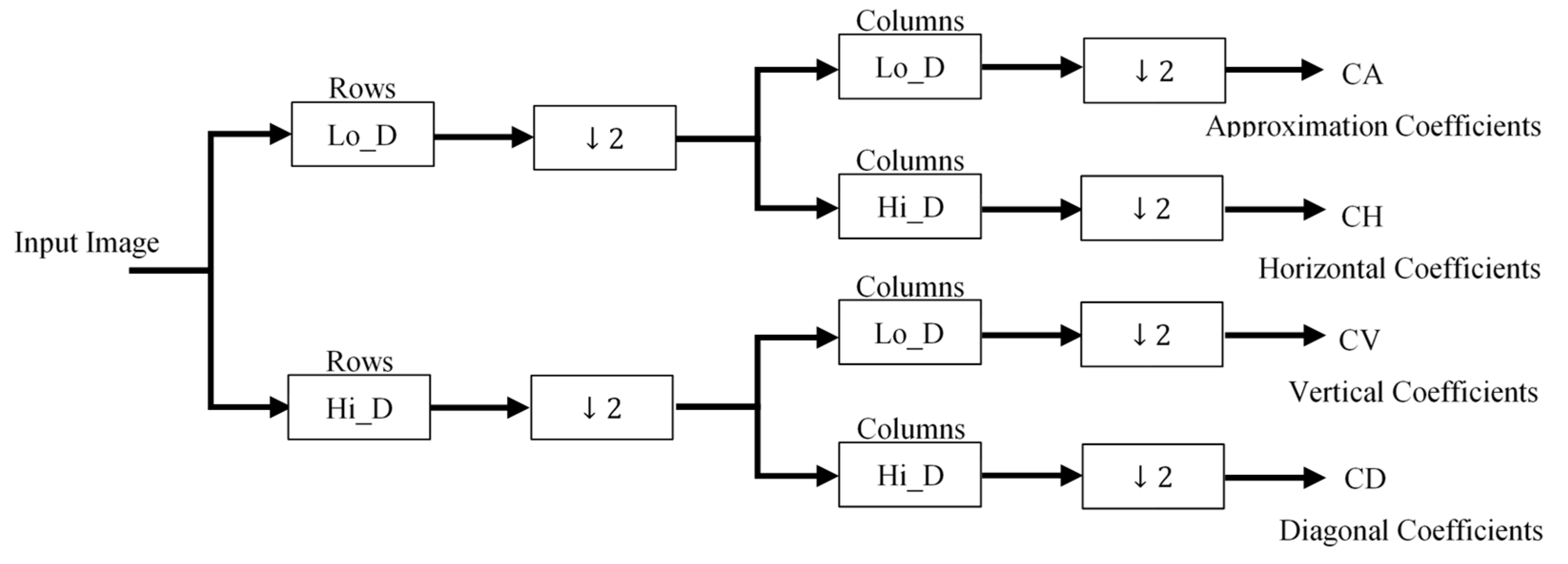
3.1. Wavelet Transforms

Wavelet Transforms were selected for preprocessing, since they examine images in a time–frequency localization, which helps to implement many methods, based on the wavelet for image processing [55]. The image was dismantled into two parts, using an LP filter and an HP filter, and each of these parts was down-sampled by two [56], as illustrated in Figure 2.

where Lo_D is a low-pass filter, Hi_D is a high-pass filter, $\downarrow 2$ denotes a down-sampling with a factor of two (keeping the even indexed rows or columns).

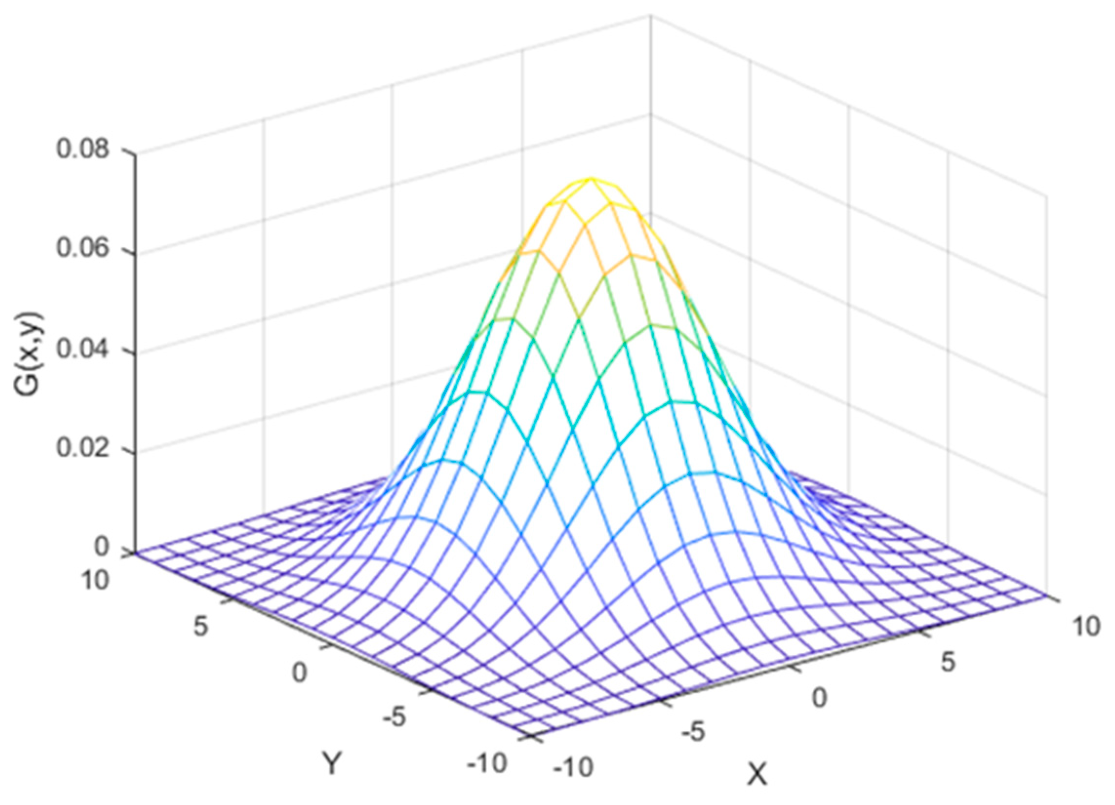
3.2. Gaussian Low-Pass Filter (GLPF)

The Gaussian Low-Pass filter or Gaussian smoothing is a filter that results in the smoothing of an image, by using a Gaussian function. It is used to filter images and reduce image noise [57].

The GLPF is used in many image processing systems that require a pre-preparing for their inputs, since it reduces the image noise [58] and allows only the lower-frequency components of the image to pass [13]. The equation of a Gaussian function in two dimensions is given by the following formula:

$$\begin{array}{cc}& G\left(x,y\right)=\frac{1}{2\pi {\sigma }^2}{e}^{-\frac{x^2+y^2}{2{\sigma }^2}}\end{array}$$

(1)

where, x and y are, respectively, the distance from the origin, in the horizontal and vertical axes, $\sigma$ represents the standard deviation of the Gaussian distribution. Figure 3 shows the Gaussian Low-Pass Filter for ($\sigma =2)$.

3.3. Difference of Gaussians (DoG)

If there are two copies of the same image and these two copies are being filtered using two Gaussian filters with different variances ${\sigma }_1^2$ and ${\sigma }_2^2$ (where ${\sigma }_2>{\sigma }_1$), to produce two new images, the result of subtracting these two new images is the DoG [59]. The filtering process is the convolution of the image with the filter kernel. Filtering the image keeps only the low-frequency spatial information. Therefore, subtracting one result from the other becomes a bandpass operation [60]. If ${\sigma }_1=\sigma$ and ${\sigma }_2=K\sigma$, then the DoG of image I, for the two-dimensional case, is the function:

$${\Gamma }_{\sigma ,K\sigma }\left(x,y\right)=I\ast \frac{1}{2\pi {\sigma }^2}{e}^{-\frac{-\left(x^2+y^2\right)}{2{\sigma }^2}}-I\ast \frac{1}{2\pi K^2{\sigma }^2}{e}^{-\frac{-\left(x^2+y^2\right)}{2K^2{\sigma }^2}}$$

(2)

where $\Gamma$ is the DoG function, I is the original image.

4. Feature Extraction Methods

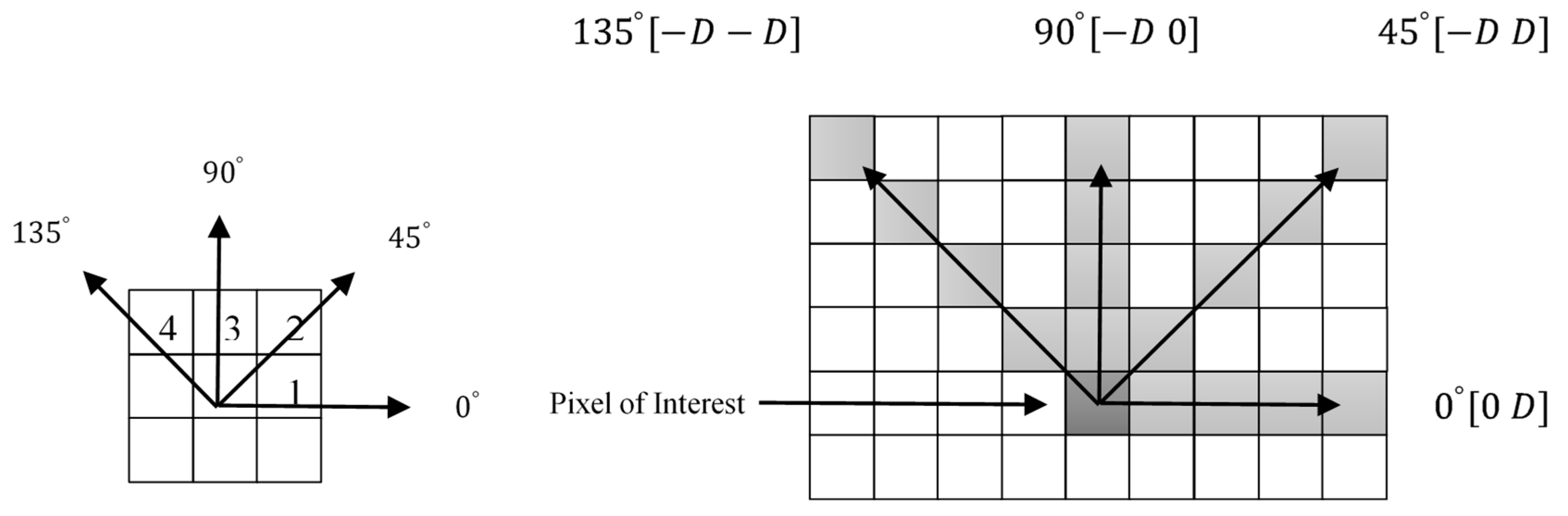
4.1. Feature Extraction Using GLCM

The GLCM is one of the methods used for feature extraction. Its concept was introduced by Harlick et al. [61]. In GLCM, the extracted features depend on the direction (angle θ) and the distance (D) from the pixel of interest [7], as illustrated in Figure 4.

In this study, a number of values (D = 1, 2, and 3 and θ = 0°, 45°, 90°, and 135°) were examined to calculate the best scenario. The used features were the correlations, contrast, maximum probability, angular second moment, mean, homogeneity, entropy, and dissimilarity [61]. These features were calculated using the following formulae:

1. Correlation:

$$f_1={\displaystyle \sum }_i{\displaystyle \sum }_j\frac{\left(i-{\mu }_x\right)\left(j-{\mu }_y\right)p\left(x,y\right)}{{\sigma }_x{\sigma }_y}$$

(3)

2. Contrast:

$$f_2={\displaystyle \sum }_i{\displaystyle \sum }_j{\left(i-j\right)}^{2}p\left(x,y\right)$$

(4)

3. Maximum probability:

$$f_3=max\left(\frac{p\left(x,y\right)}{\left|i\times j\right|}\right)$$

(5)

4. Angular Second Moment:

$$f_4={\displaystyle \sum }_i{\displaystyle \sum }_{j}p{\left(x,y\right)}^2$$

(6)

5. Mean:

$$f_5=\frac{\sum p\left(x,y\right)}{i\times j}$$

(7)

6. Homogeneity:

$$f_6={\displaystyle \sum }_i{\displaystyle \sum }_j\left(\frac{p\left(x,y\right)}{1+\left|i-j\right|}\right)$$

(8)

7. Entropy:

$$f_7={\displaystyle \sum }_i{\displaystyle \sum }_j\left(\frac{p\left(x,y\right)}{\log p\left(x,y\right)}\right)$$

(9)

8. Dissimilarity:

$$f_8={\displaystyle \sum }_i{\displaystyle \sum }_j\left|i-j\right|p\left(x,y\right)$$

(10)

where ${\mu }_x$ is the mean of the column values in the image, ${\mu }_y$ is the mean of the row values in the image, p(x,y) denotes the elements of the Gray Level Co-Occurrence Matrix, i and j are, respectively, the lengths of the row and column of the image [61].

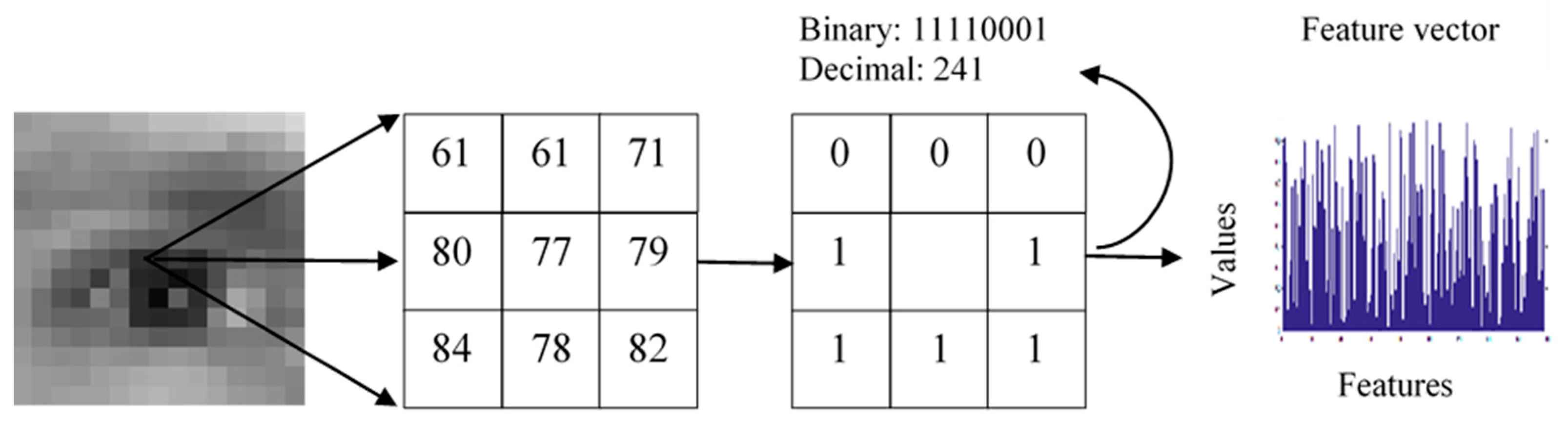
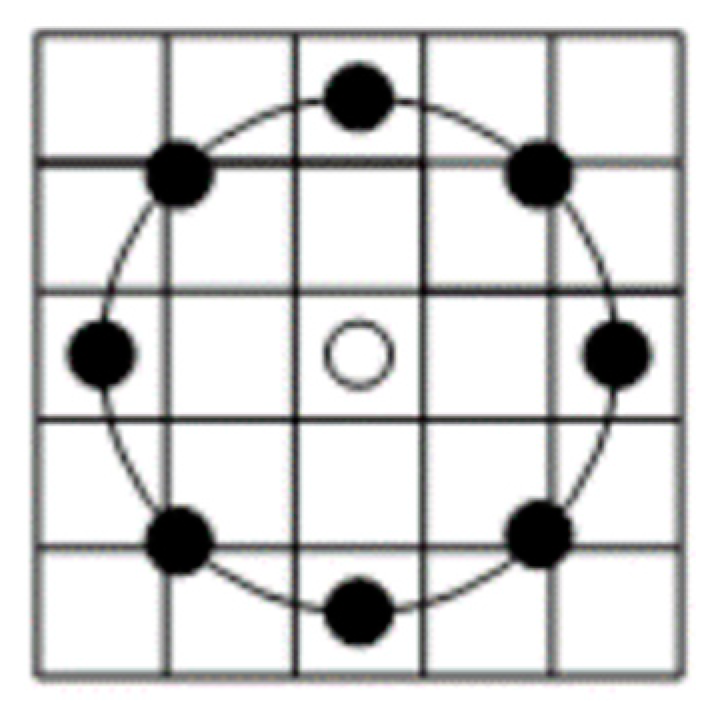
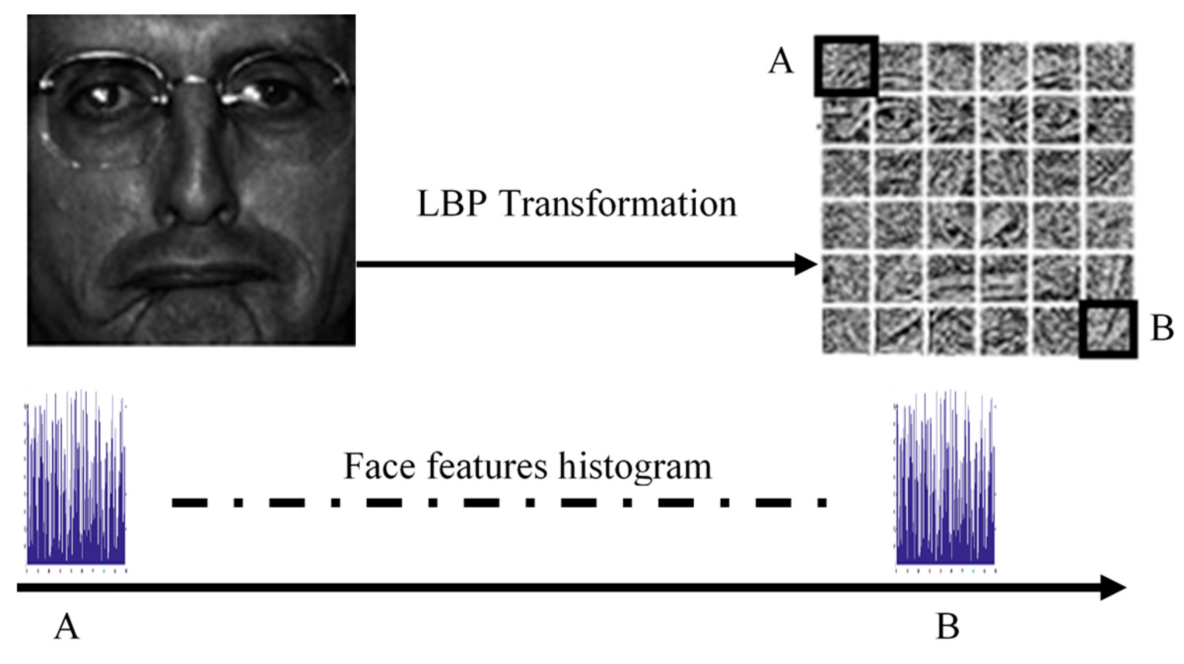
4.2. Feature Extraction Using LBP

One of the most widely used methods to analyze and model texture is the LBP method [9]. It could be basically described as a 3 × 3 square operator. In each square, the eight‑neighborhood pixels were compared with the one in the center. If the pixel values of the neighbors were greater than or equal to the pixel value at the center, they were replaced by 1. If not, then their values were replaced by 0. Then, the new binary values of the neighbors were concatenated to produce one decimal value that was considered to be a new value for the pixel in the center. The window was passed to the next pixel and the same operation was repeated. These new decimal values represented the histogram of the input texture. Equation (11) described the algorithm of the LBP operation:

$${\mathrm{LBP}}_{{\mathrm{N}}_P,\mathrm{R}\left(x,y\right)}={{\displaystyle \sum }}_{{\mathrm{N}}_P=0}^{{\mathrm{N}}_P-1}\mathrm{s}\left({\mathrm{g}}_{\mathrm{p}}-{\mathrm{g}}_{\mathrm{c}}\right)2^{{\mathrm{N}}_P}$$

(11)

where s is the sign function, ${\mathrm{N}}_P$ is the number of neighborhood pixels, g_p represents the gray level value of the neighboring pixels, and g_c represents the gray level value of the central pixels. 2^P is required to produce decimal values.

The traditional LBP [6] analyzes the texture of the image and thresholds a 3 × 3 square neighborhood as the center pixel value. It only uses the sign information to produce the LBP, as illustrated in Figure 5 [4].

In a newer implementation, the LBP operation has been upgraded to deal with any neighborhood size, by replacing the square with a circle [9]. This can be described by (${\mathrm{N}}_P$,R), where R is the radius of the circle used. Figure 6 illustrates an (8, 2) neighborhood. Additionally, there are a number of other modifications to the LBP [4].

The term $LB{P}_{P,R}^{u^2}$ is used to describe the LBP operation, where u² denotes the use of a uniform pattern. The resulting histogram results in the necessary information distributed in the image, such as edges, corners, uniform areas, etc. The effective operation must take care of the spatial information in the image, during the representation. One strategy to accomplish this is to partition the image into a number of small areas $R_0,R_1,\dots , R_{m-1}$ [6], where $m$ is the number of areas. If the size of the histogram is B, then the length of the feature vector is mB. It is obvious from this relation that the number of areas m determines the length of the feature vector, which means selecting small areas results in long feature vectors, leading to extreme use of memory and a slow classification processing. Selecting large areas causes a loss of spatial information. An example of a preprocessed face image partitioned into thirty-six windows and the resulting face feature histogram are illustrated in Figure 7 [62].

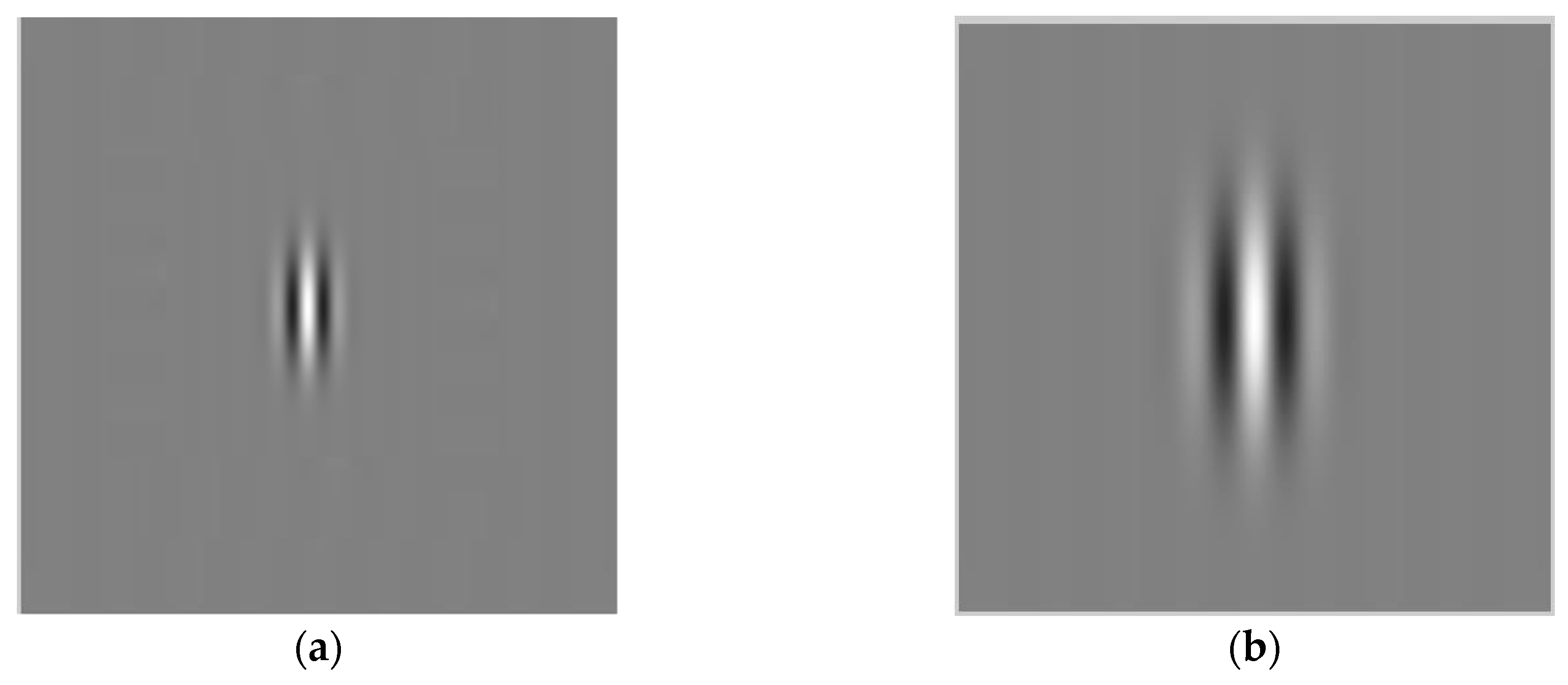
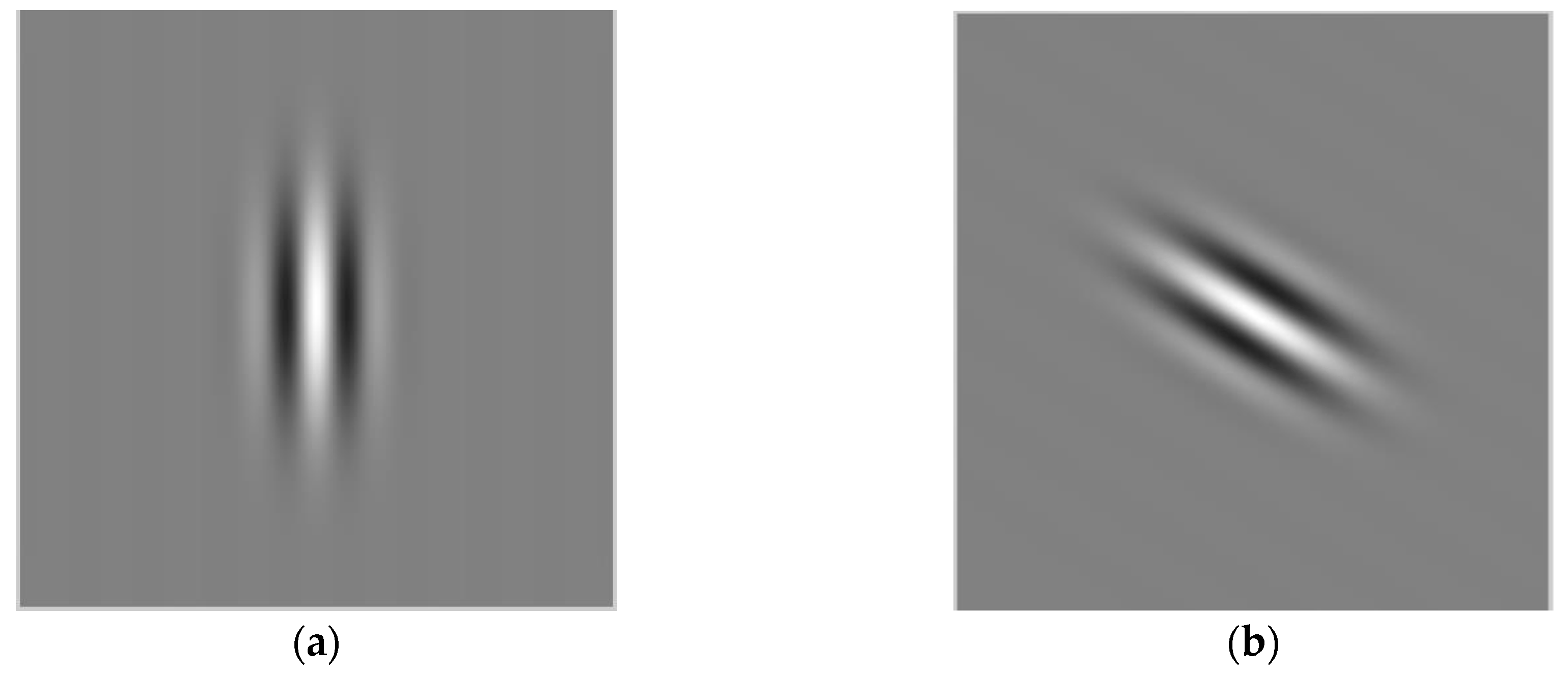
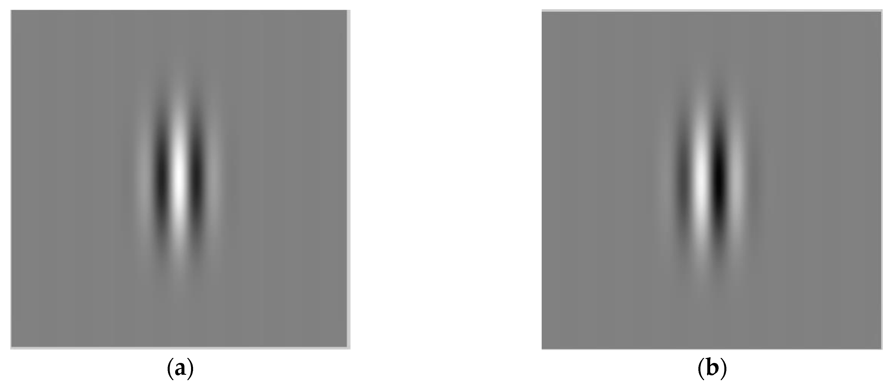
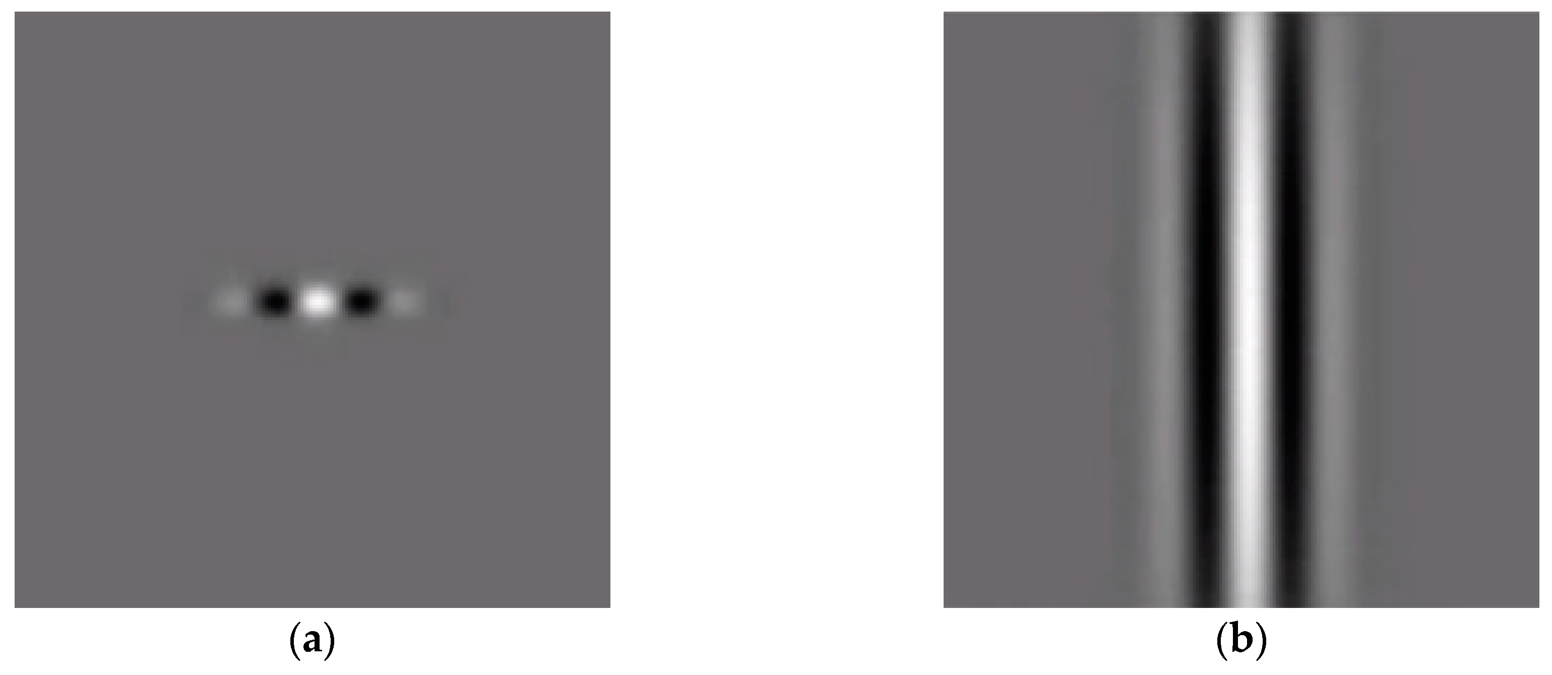
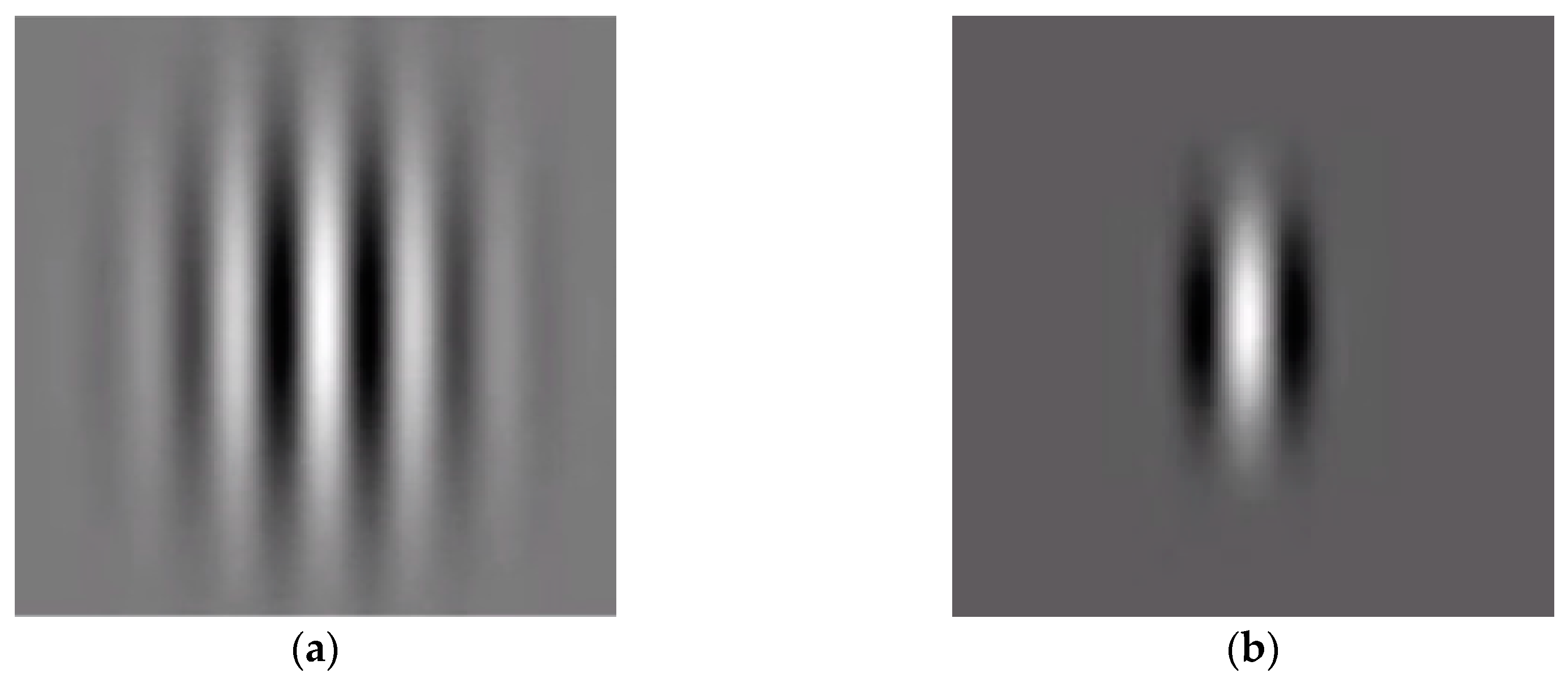
4.3. Feature Extraction Using the Gabor Filter

The Gabor filter is a very helpful tool in image processing, especially in FR [63]. In the spatial domain, the Gabor filter with two dimensions is the modulation of a Gaussian kernel function, by a complex sinusoidal plane wave with a center frequency f and orientation θ [64], and is defined as:

$$\begin{gathered} G\left(x,y\right)=\frac{f^2}{\pi \gamma \eta }{e}^{\left(-\frac{x^{\prime 2}+{\gamma }^2{y}^{\prime 2}}{2{\sigma }^2}\right)}{e}^{\left(j2\pi f{x}^{\prime }+\varphi \right)} \\ {x}^{\prime }=x\cos \theta +y\sin \theta \\ {y}^{\prime }=-x\sin \theta +y\cos \theta \end{gathered}$$

(12)

where γ and η denote the ratio between the envelope of the Gaussian function with standard deviation σ and the center frequency, and ϕ defines the phase offset.

The frequency (or wavelength) governs the width of the stripes in the function, and by increasing the frequency, the stripes become thinner. The orientation governs the rotation of the Gabor envelope and the aspect ratio controls the height of the function. For a very large aspect ratio, the envelope approaches a height of one pixel, and for a very small aspect ratio, the height stretches across the image. The bandwidth controls the overall size of the Gabor envelope, such that for a large bandwidth, the envelope increases, allowing more stripes [65].

Figure 8, Figure 9, Figure 10, Figure 11 and Figure 12 show the effect of changing some parameters for the function of a Gabor.

Gabor filters have many advantages, such as invariance to rotation, scale, and translation. Moreover, they are robust against disturbances in images, such as change in illumination [66,67], and they have been found to be particularly appropriate to extract many features from an image, using different frequencies and orientation for Gabor filters [65].

They are useful, especially in feature extraction for texture analysis and segmentation. The varying orientation observes the texture that is oriented in a particular direction, while the varying Gaussian envelope standard deviation controls the region size of the image that is being analyzed [68].

5. Classification

Although there were many classifiers used for the classification, such as the Euclidean Distance, the Cosine Distance, Linear Discriminant Analysis, Quadratic Discriminant Analysis, Learning Vector Quantization, and Support Vector Machines [69]. The Minimum Euclidean Distance classifier was considered to be one of the most popular classifiers that could be easily designed [70] and widely used [71,72]. In general, it was used to examine the similarities between objects. In this study, we used the k-nearest neighbor classifier (for k = 1) with a Euclidean distance function as a distance metric.

5.1. Euclidean Distance

The Euclidean distance d between two points i and j, where I = (i₁, i₂,..., i_n) and j = (j₁, j₂,..., j_n), in Cartesian coordinates, is the length of the straightest line between them. This distance is given by the formula:

$$d\left(i,j\right)=\sqrt{{\left(i_1-j_1\right)}^2+{\left(i_2-j_2\right)}^2+\dots +{\left(i_n-j_n\right)}^2}=\sqrt{{\displaystyle \sum }_{k=1}^n{\left(i_k-j_k\right)}^2}$$

(13)

Therefore, if the two points are close to each other, then the value of d is small; otherwise, it is large. The Euclidean vector is the location of a point in a Euclidean n‑space, where the length of this vector is measured by the formula of the Euclidean norm, given by:

$$\Vert I\Vert =\sqrt{i_1^2+i_2^2+\dots +i_n^2}$$

(14)

This tool is used to test how similar one object (face) is to another, by testing the similarities between their respective feature vectors.

6. Dataset

The dataset in this study was taken from the ORL and Yale datasets.

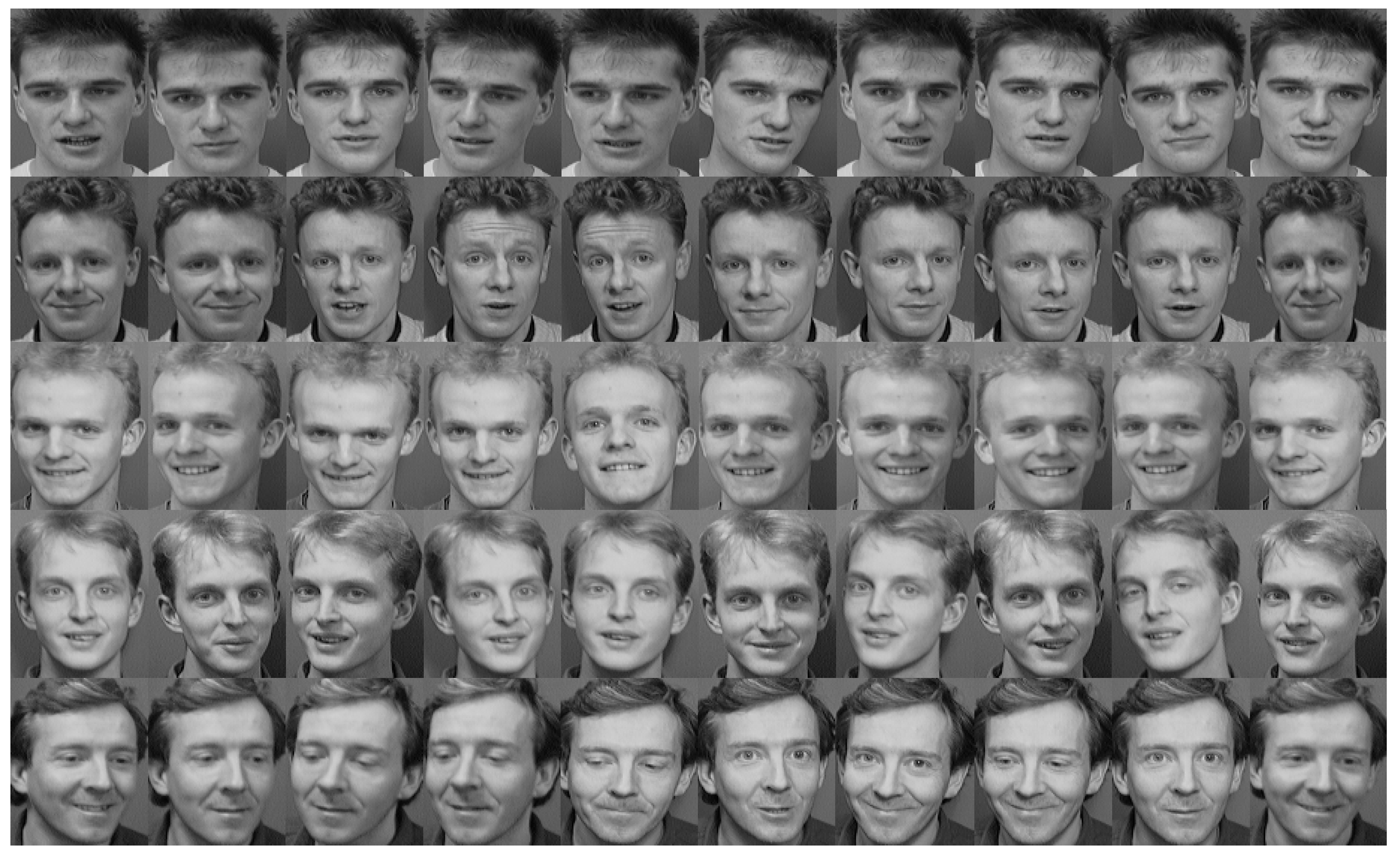
6.1. The ORL Dataset

The ORL is a well-known face dataset that is used to test FR algorithms. It has 400 images of 40 distinct persons, 10 images for each person. The dataset is varied in many aspects. First, the images are taken at different times during the lives of the people. Second, the images include different variations and different facial expressions, such as closed or open eyes. Some of the people are smiling, others are not. In addition, there are a number of people wearing spectacles while others are not wearing spectacles. Furthermore, a number of the images include up to twenty degrees of tilting and rotation of the face [3].

A number of face images from the ORL dataset are illustrated in Figure 13.

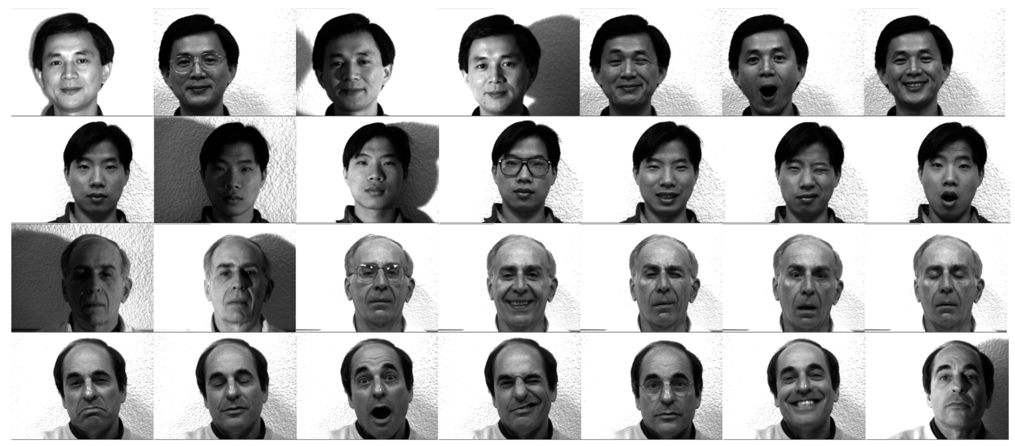
6.2. The Yale Dataset

In this dataset, there exists 165 images for 15 unique people, 11 images for each person with different cases, such as normal, sad, sleepy, etc. The dataset includes many variations of pose, illumination, and expression [3]. A number of images from the Yale dataset are illustrated in Figure 14.

7. Experiments and Results

This section shows some results obtained from simulations using MATLAB 2015b. The experiments were implemented on images from the ORL and Yale datasets, using the proposed method. The proposed method was compared with the performance of PCA [26], Collaborative Representation-Based Classification (CRC) [73], SRC [21], and SCRC [3,54].

The FR system consisted of three stages. The first stage was the Preprocessing Stage, in which the 2‑D DWT, the GLPF, and the DoG were used separately. The second stage was the Feature Extraction Stage, where the LBP, the GLCM, and the Gabor Filter were examined; all these algorithms were first tested separately, then, the two methods from the list were combined in the Feature Extraction Stage. In the final stage (the Classification Stage), the Euclidean distance was used as a classifier. The procedure was carried out and tested using the Original Training Samples (OTS) and the Original with Symmetrical Training Samples (OSTS) from the ORL and the Yale datasets.

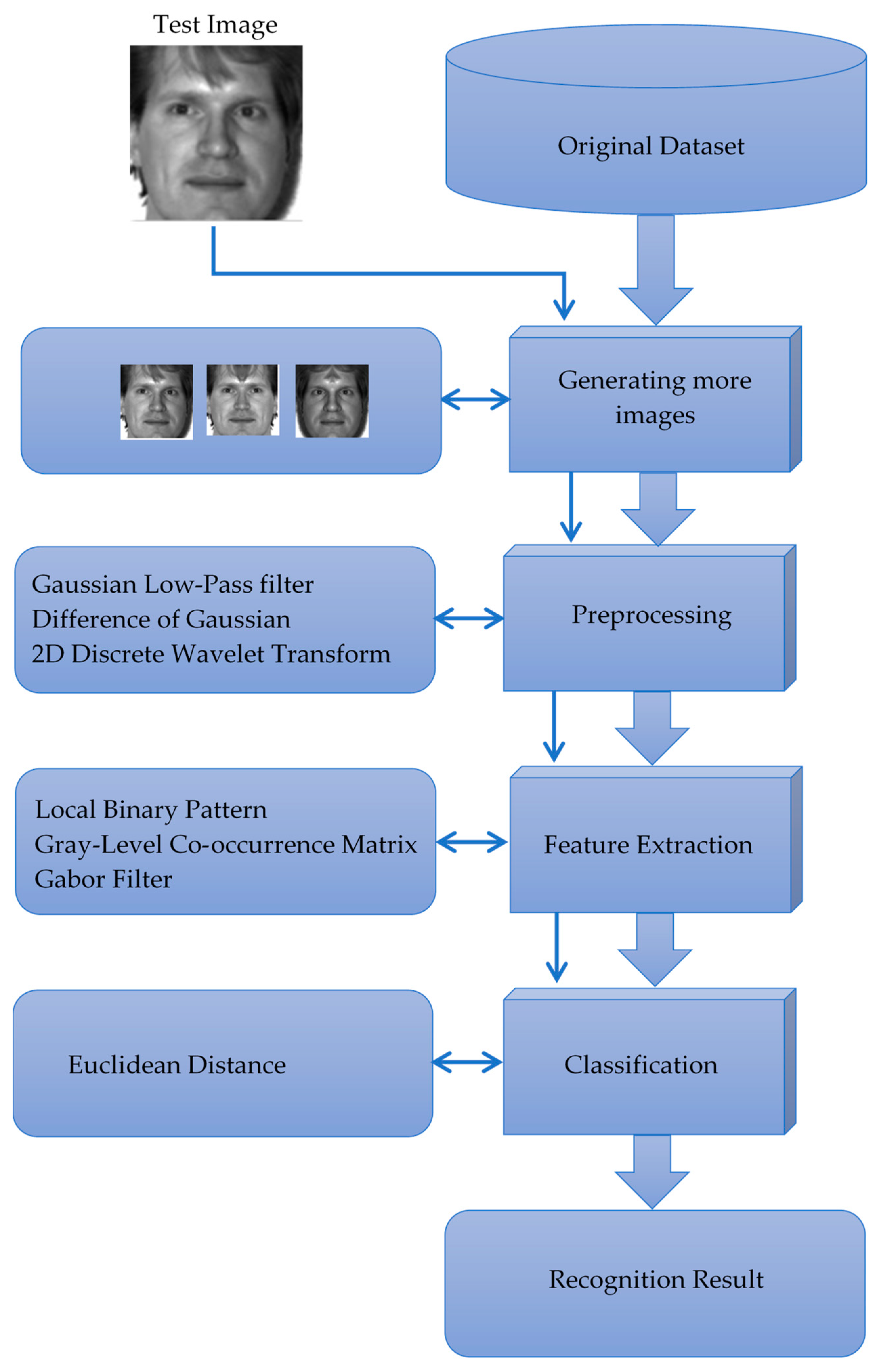
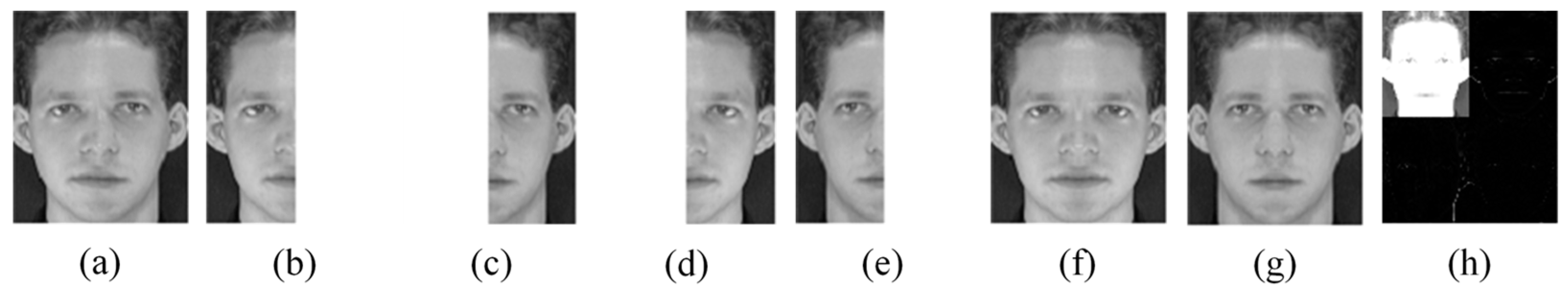
7.1. Generating New Images

In order to increase the size of the training data, new training images were generated using the property of face symmetry, since those images reflect some part of the face that is not shown by the original images, as illustrated in Figure 15.

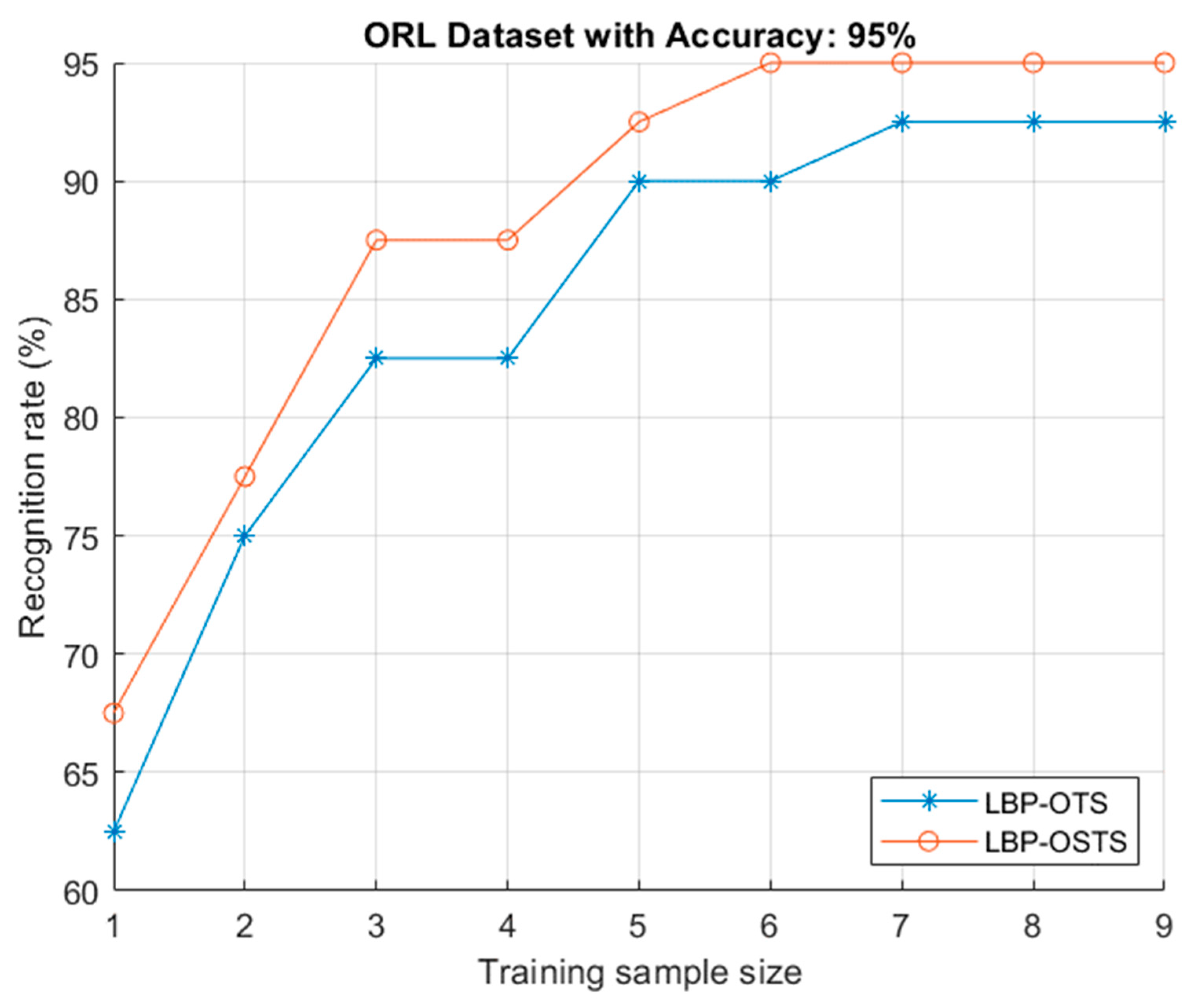
7.2. Experiments on the ORL Dataset

In the experiment, one, two, up to nine face images of each person from the ORL dataset with size 112 × 92 were used, respectively, as the training samples and the rest of images were used as the testing samples. The features of the training and testing images were extracted using the LBP, the GLCM, and the Gabor Filter. Each image had one feature vector,$f=\left[f_1, f_2\cdots f_m\right]$, where m is the number of one-image features.

The feature vector of the test image was compared with the feature vectors of the training images, using the Euclidean distance classifier. The person who had a training image feature vector with a minimum Euclidean distance was considered to be the result of recognition. The experiments were run ten times, with random image selection in each experiment. The recognition rate was calculated as the average of each set of these experiments.

7.3. Experiments on Symmetrical ORL Dataset

In this experiment, the original and symmetrical images were used for training. The experiment revealed the use of symmetrical images, along with the original images, improved the accuracy of FR, as compared to only using the original images as training samples. Figure 16 shows the results of using the LBP for feature extraction with OTS and OSTS.

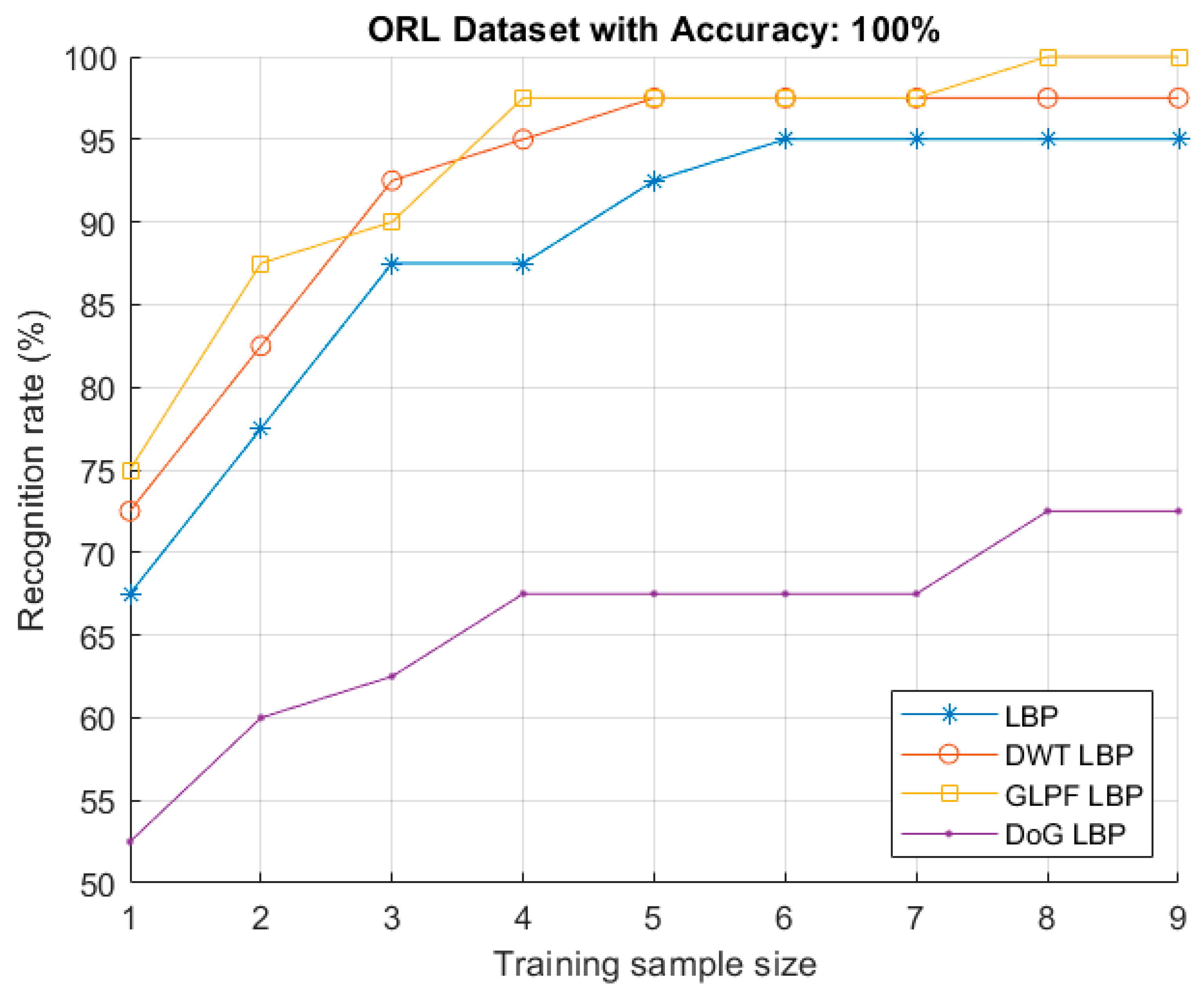
7.4. Using a Preprocessing Stage

In this experiment, three different methods for preprocessing were separately examined with LBP. First, LBP was used without any preprocessing stage, followed by the GLPF being used for the preprocessing stage, with a standard deviation of σ = 1 and a window size of 5 pixels. Then the DoG with σ₁ = 0.1, σ₂ = 2.0, and a window size of 5 pixels was used for the preprocessing stage. Finally, the 2‑D DWT was also used for the preprocessing stage.

The results showed that the use of GLPF or 2‑D DWT as a preprocessing stage improved the accuracy of FR, as compared to not using any of the preprocessing stages, as in Figure 17. The experiments were implemented using OSTS.

7.5. The GLCM Method

In this experiment, the GLCM method was used to extract the features. The parameters of the GLCM method were selected to be D = 1 and θ = 0°.

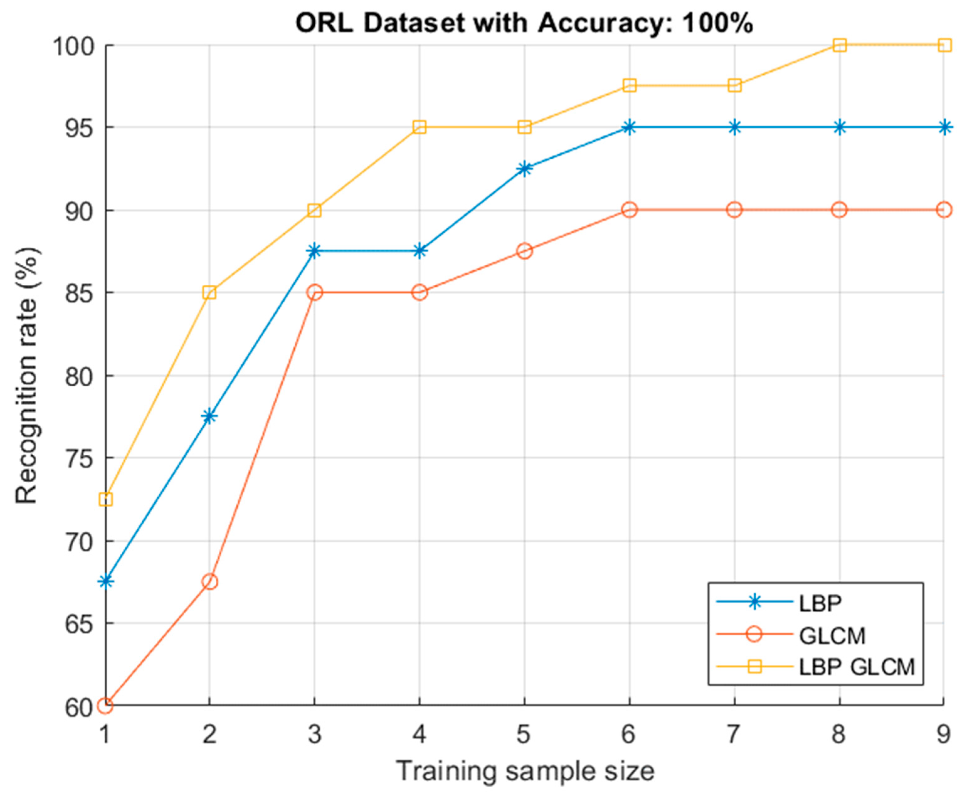
7.6. Combining Feature Extraction Methods

In this experiment, two methods were used separately for feature extraction—the LBP and the GLCM. Then, the two feature vectors obtained from these two methods were normalized and concatenated to produce one longer feature vector, which was used for training and testing. The results showed that the combination of the two methods could help to improve the accuracy of FR, as compared to using one method for feature extraction, as shown in Figure 18. The experiments were implemented using OSTS.

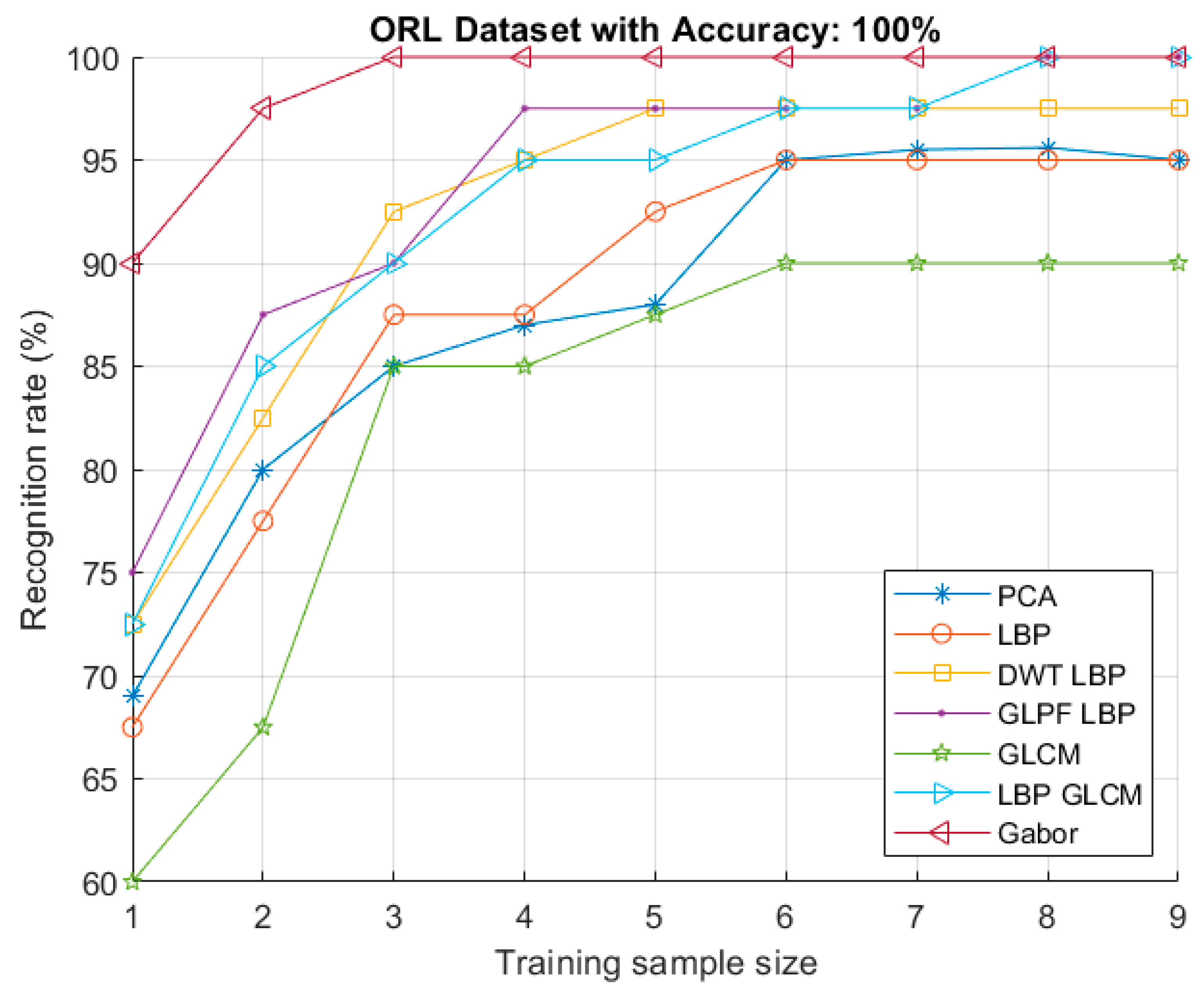
7.7. The Gabor Filter Method

In this experiment, the Gabor Filter was examined to extract the features. The parameters of the Gabor filter bank were set as following. The number of scales was set to 5, the number of orientations was set to 8, and the number of rows and columns in a 2-D Gabor filter were each set to 39. Additionally, the parameter of the Gabor function was set as following. The factor of down-sampling along the rows was set to 4 and the factor of down-sampling along the columns was set to 4. The experiment revealed that the best results were obtained using the Gabor Filter, as compared to the other methods. Figure 19 shows the results of the recognition rates for different methods on the OSTS–ORL dataset. These methods were—the LBP without any preprocessing stage (LBP), the LBP with DWT as a preprocessing stage (DWT-LBP), the LBP with GLPF as a preprocessing stage (GLPF-LBP), the GLCM, the LBP combined with the GLCM and the Gabor. For the sake of comparison, the performance of the PCA has also been shown in the figure.

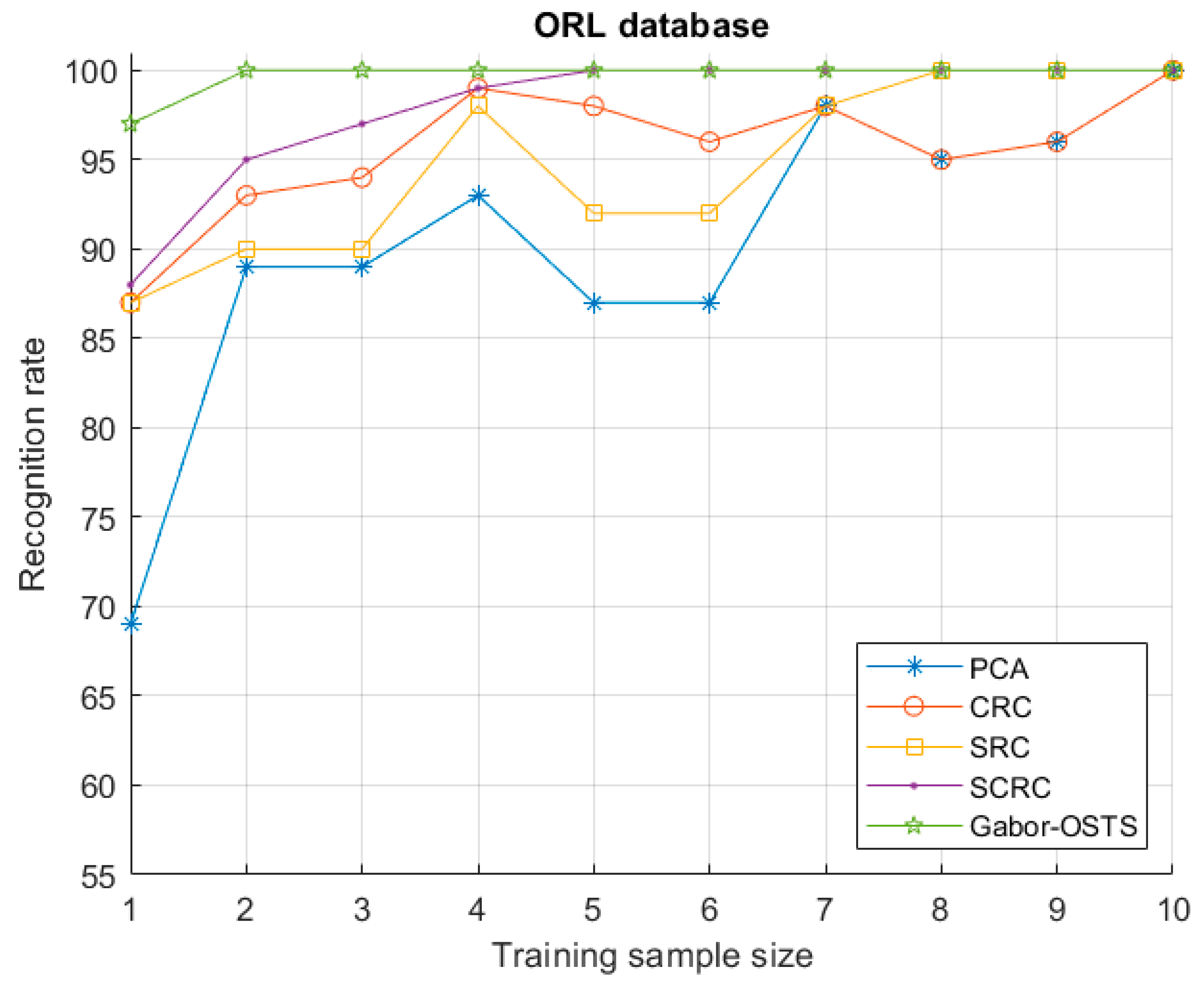
7.8. Other Experiments

In order to generalize the proposed method, various cases and situations were examined and studied. For this purpose, different experiments were carried out, using different preprocessing techniques and different feature extraction methods. These experiments were implemented to compare the performance of the FR system when the original training samples (OTS) was used alone and when the original training samples were used, along with the symmetrical training samples (OSTS). For the sake of completeness, the results were compared with the methods in the literature. All obtained results have been summarized in

Table 1. The recognition rates of the different methods on the ORL dataset, using the OTS compared with the OSTS.

Preprocessing Method	Feature Extraction Method		No. of Training Images
			1	2	3	4	5	6	7	8	9
			Recognition Rate %
No	LBP	OTS	62.5	75	82.5	82.5	90	90	92.5	92.5	92.5
		OSTS	67.5	77.5	87.5	87.5	92.5	95	95	95	95
DWT	LBP	OTS	70	80	90	92.5	95	95	95	97.5	97.5
		OSTS	72.5	82.5	92.5	95	97.5	97.5	97.5	97.5	97.5
GLPF	LBP	OTS	72.5	80	87.5	92.5	95	95	97.5	97.5	97.5
		OSTS	75	87.5	90	97.5	97.5	97.5	97.5	100	100
DoG	LBP	OTS	50	55	62.5	62.5	65	65	65	67.5	70
		OSTS	52.5	60	62.5	67.5	67.5	67.5	67.5	72.5	72.5
No	GLCM	OTS	55	65	77.5	77.5	80	87.5	87.5	87.5	90
		OSTS	60	67.5	85	85	87.5	90	90	90	90
DWT	GLCM	OTS	50	55	60	60	62.5	62.5	62.5	65	62.5
		OSTS	57.5	70	70	80	77.5	75	80	80	82.5
DoG	GLCM	OTS	37.5	40	40	40	42.5	42.5	45	45	45
		OSTS	40	42.5	50	50	50	50	50	52.5	55
GLPF	GLCM	OTS	57.5	67.5	80	80	80	82.5	82.5	82.5	82.5
		OSTS	57.5	75	82.5	82.5	87.5	90	90	90	90
No	LBP–GLCM	OTS	70	82.5	87.5	92.5	92.5	95	95	95	95
		OSTS	72.5	85	90	95	95	97.5	97.5	100	100
No	Gabor	OTS	87.5	95	100	100	100	100	100	100	100
		OSTS	90	97.5	100	100	100	100	100	100	100
No	PCA	OTS	69	79	84	87	89	95	96	96	95
No	CRC	OTS	72	84	86	91	91	94	93	94	93
No	SRC	OTS	76	89	90	94	94	94	95	96	95
No	SCRC	OSTS	76	90	92	94	94	95	96	96	95

.

7.9. Experiments on the Yale Dataset

In this experiment, from the Yale dataset, either one, two, or up to ten facial images of size 154 × 154, were chosen for each person, which were then used as the training samples, and the rest of images were used as the testing samples. These experiments were similar in procedure to those in the ORL dataset, where a variety of methods were tested for preprocessing and feature extraction. These methods were tested and examined using the OTS and the OSTS. Many results were obtained using the different cases, these results have been summarized in

Table 2. The recognition rates of the different methods on the Yale dataset, using the OTS and the OSTS.

Preprocessing Method	Feature Extraction Method		No. of Training Images
			1	2	3	4	5	6	7	8	9	10
			Recognition Rate %
No	LBP	OTS	90	93	96	98	100	100	100	100	100	100
		OSTS	95	98	100	100	100	100	100	100	100	100
No	GLCM	OTS	70	75	87	87	87	87	87	87	87	87
		OSTS	75	80	93	93	93	93	93	93	93	93
DWT	GLCM	OTS	12	15	18	20	20	20	20	20	20	20
		OSTS	20	23	27	30	33	33	33	33	33	33
DoG	GLCM	OTS	60	60	73	73	73	73	80	80	80	80
		OSTS	65	67	87	87	87	87	87	87	87	87
GLPF	GLCM	OTS	80	85	87	87	87	87	87	87	87	87
		OSTS	80	93	93	93	93	93	93	93	93	93
No	Gabor	OTS	95	97	100	100	100	100	100	100	100	100
		OSTS	97	100	100	100	100	100	100	100	100	100
No	PCA	OTS	69	89	89	93	87	87	98	95	96	100
No	CRC	OTS	87	93	94	99	98	96	98	95	96	100
No	SRC	OTS	87	90	90	98	92	92	98	100	100	100
No	SCRC	OSTS	88	95	97	99	100	100	100	100	100	100

and Figure 20, along with the performance of the methods in the literature.

8. Conclusions

This paper presents an effective method to overcome the restricted number of training sets using the property of face symmetry. The use of this property also reduced the effect of illumination and pose variations. First, a new set of face images was generated using the left and right halves of each face. Second, the original and generated samples were preprocessed using the 2‑D DWT, GLPF, and DoG; then the features of these samples were extracted using the LBP, the GLCM, and the Gabor filter methods. Finally, the Euclidean classifier was used to obtain the results of the recognition. The use of the GLCM alone is not recommended, but it could support the performance of the LBP by using the combined features from both methods. It could be well-observed that combining features from different methods provided a better performance, as opposed to using a single method. The Gabor filter was indeed a very helpful tool in FR. This paper also showed that the use of the preprocessing stage in the recognition system improved the accuracy of FR, as compared to not using any of the preprocessing stages. Although the method was especially effective when the set of training samples was small, it took more time to process the increased number of training samples.

References

1. Ahonen, T.; Hadid, A.; Pietikainen, M. Face description with local binary patterns: Application to face recognition. IEEE Trans. Pattern Anal. Mach. Intell. 2006, 28, 2037–2041. [Google Scholar] [CrossRef] [PubMed]
2. Tan, X.; Chen, S.; Zhou, Z.-H.; Zhang, F. Face recognition from a single image per person: A survey. Pattern Recognit. 2006, 39, 1725–1745. [Google Scholar] [CrossRef] [Green Version]
3. Liu, Z.; Pu, J.; Wu, Q.; Zhao, X. Using the original and symmetrical face training samples to perform collaborative representation for face recognition. Optik 2016, 127, 1900–1904. [Google Scholar] [CrossRef]
4. Liu, L.; Fieguth, P.; Guo, Y.; Wang, X.; Pietikäinen, M. Local binary features for texture classification: Taxonomy and experimental study. Pattern Recognit. 2017, 62, 135–160. [Google Scholar] [CrossRef]
5. Julsing, B. Face Recognition with Local Binary Patterns; Research No. SAS008-07; University of Twente: Enschede, The Netherlands, 2007. [Google Scholar]
6. Ahonen, T.; Hadid, A.; Pietikäinen, M. Face recognition with local binary patterns. In Computer Vision-Eccv 2004, 2nd ed.; Springer: Berlin, Germany, 2004; pp. 469–481. [Google Scholar]
7. Yang, P.; Yang, G. Feature extraction using dual-tree complex wavelet transform and gray level co-occurrence matrix. Neurocomputing 2016, 197, 212–220. [Google Scholar] [CrossRef]
8. Sun, Y.; Yu, J. Facial Expression Recognition by Fusing Gabor and Local Binary Pattern Features. In Proceedings of the International Conference on Multimedia Modeling, Reykjavik, Iceland, 4–6 January 2017; pp. 209–220. [Google Scholar]
9. Ojala, T.; Pietikäinen, M.; Mäenpää, T. Multiresolution gray-scale and rotation invariant texture classification with local binary patterns. IEEE Trans. Pattern Anal. Mach. Intell. 2002, 24, 971–987. [Google Scholar] [CrossRef] [Green Version]
10. Arabi, P.M.; Joshi, G.; Deepa, N.V. Performance evaluation of glcm and pixel intensity matrix for skin texture analysis. Perspect. Sci. 2016, 8, 203–206. [Google Scholar] [CrossRef]
11. Li, W.; Mao, K.; Zhang, H.; Chai, T. Designing compact gabor filter banks for efficient texture feature extraction. In Proceedings of the 2010 11th International Conference on Control Automation Robotics & Vision, Singapore, 7–10 December 2010; pp. 1193–1197. [Google Scholar]
12. Tan, X.; Triggs, B. Fusing gabor and lbp feature sets for kernel-based face recognition. In Proceedings of the International Workshop on Analysis and Modeling of Faces and Gestures, Rio de Janeiro, Brazil, 20 October 2007; pp. 235–249. [Google Scholar]
13. Makandar, A.; Halalli, B. Image enhancement techniques using highpass and lowpass filters. Int. J. Comput. Appl. 2015, 109, 21–27. [Google Scholar] [CrossRef]
14. Anila, S.; Devarajan, N. Preprocessing technique for face recognition applications under varying illumination conditions. Glob. J. Comput. Sci. Technol. 2012, 12, 12–18. [Google Scholar]
15. Jadhav, D.V.; Holambe, R.S. Feature extraction using radon and wavelet transforms with application to face recognition. Neurocomputing 2009, 72, 1951–1959. [Google Scholar] [CrossRef]
16. Samaria, F.S.; Harter, A.C. Parameterisation of a stochastic model for human face identification. In Proceedings of the Second IEEE Workshop on Applications of Computer Vision, Sarasota, FL, USA, 5–7 December 1994; pp. 138–142. [Google Scholar] [Green Version]
17. Georghiades, A.; Belhumeur, P.; Kriegman, D. Yale Face Database. Center for Computational Vision and Control at Yale University, 1997. Available online: http://cvc.cs.yale.edu/cvc/projects/yalefaces/yalefaces.html (accessed on 31 October 2016).
18. Azeem, A.; Sharif, M.; Raza, M.; Murtaza, M. A survey: Face recognition techniques under partial occlusion. Int. Arab J. Inf. Technol. 2014, 11, 1–10. [Google Scholar]
19. Mehta, G.; Vatta, S. An introduction to a face recognition system using pca, flda and artificial neural networks. Int. J. Adv. Res. Comput. Sci. Softw. Eng. 2013, 3, 1418–1420. [Google Scholar]
20. Zhao, W.; Chellappa, R.; Phillips, P.J.; Rosenfeld, A. Face recognition: A literature survey. ACM Comput. Surv. (CSUR) 2003, 35, 399–458. [Google Scholar] [CrossRef]
21. Wright, J.; Yang, A.Y.; Ganesh, A.; Sastry, S.S.; Ma, Y. Robust face recognition via sparse representation. IEEE Trans. Pattern Anal. Mach. Intell. 2009, 31, 210–227. [Google Scholar] [CrossRef] [PubMed]
22. Yang, M.; Zhang, L. Gabor feature based sparse representation for face recognition with gabor occlusion dictionary. In Computer Vision–Eccv 2010; Springer: Berlin, Germany, 2010; pp. 448–461. [Google Scholar]
23. Mairal, J.; Ponce, J.; Sapiro, G.; Zisserman, A.; Bach, F.R. Supervised dictionary learning. In Proceedings of the Advances in Neural Information Processing Systems, Vancouver, BC, Canada, 7–10 December 2009; pp. 1033–1040. [Google Scholar]
24. He, X.; Yan, S.; Hu, Y.; Niyogi, P.; Zhang, H.-J. Face recognition using laplacianfaces. IEEE Trans. Pattern Anal. Mach. Intell. 2005, 27, 328–340. [Google Scholar] [PubMed]
25. Belhumeur, P.N.; Hespanha, J.P.; Kriegman, D.J. Eigenfaces vs. Fisherfaces: Recognition using class specific linear projection. IEEE Trans. Pattern Anal. Mach. Intell. 1997, 19, 711–720. [Google Scholar] [CrossRef]
26. Turk, M.A.; Pentland, A.P. Face recognition using eigenfaces. In Proceedings of the IEEE Computer Society Conference on Computer Vision and Pattern Recognition, Maui, HI, USA, 3 June 1991; pp. 586–591. [Google Scholar]
27. Tunç, B.; Gökmen, M. Manifold learning for face recognition under changing illumination. Telecommun. Syst. 2011, 47, 185–195. [Google Scholar] [CrossRef]
28. Tran, C.K.; Tseng, C.D.; Lee, T.F. In Improving the face recognition accuracy under varying illumination conditions for local binary patterns and local ternary patterns based on weber-face and singular value decomposition. In Proceedings of the 2016 3rd International Conference on Green Technology and Sustainable Development (GTSD), Kaohsiung, Taiwan, 24–25 November 2016; pp. 5–9. [Google Scholar]
29. Wiskott, L.; Fellous, J.-M.; Kuiger, N.; Von Der Malsburg, C. Face recognition by elastic bunch graph matching. IEEE Trans. Pattern Anal. Mach. Intell. 1997, 19, 775–779. [Google Scholar] [CrossRef] [Green Version]
30. Georghiades, A.S.; Belhumeur, P.N.; Kriegman, D.J. From few to many: Illumination cone models for face recognition under variable lighting and pose. IEEE Trans. Pattern Anal. Mach. Intell. 2001, 23, 643–660. [Google Scholar] [CrossRef]
31. Shashua, A.; Riklin-Raviv, T. The quotient image: Class-based re-rendering and recognition with varying illuminations. IEEE Trans. Pattern Anal. Mach. Intell. 2001, 23, 129–139. [Google Scholar] [CrossRef]
32. Zhou, S.; Chellappa, R. Rank constrained recognition under unknown illuminations. In Proceedings of the IEEE International Workshop on Analysis and Modeling of Faces and Gestures, Nice, France, 17 October 2003; pp. 11–18. [Google Scholar]
33. Zhang, L.; Samaras, D. Face recognition from a single training image under arbitrary unknown lighting using spherical harmonics. IEEE Trans. Pattern Anal. Mach. Intell. 2006, 28, 351–363. [Google Scholar] [CrossRef] [PubMed] [Green Version]
34. Lu, Z.; Zhang, L. Face recognition algorithm based on discriminative dictionary learning and sparse representation. Neurocomputing 2016, 174, 749–755. [Google Scholar] [CrossRef]
35. Kim, T.-K.; Kittler, J. Locally linear discriminant analysis for multimodally distributed classes for face recognition with a single model image. IEEE Trans. Pattern Anal. Mach. Intell. 2005, 27, 318–327. [Google Scholar] [PubMed] [Green Version]
36. Jaiswal, S. Comparison between face recognition algorithm-eigenfaces, fisherfaces and elastic bunch graph matching. Int. J. Glob. Res. Comput. Sci. 2011, 2, 187–193. [Google Scholar]
37. Pentland, A.; Moghaddam, B.; Starner, T. View-based and modular eigenspaces for face recognition. In Proceedings of the 1994 IEEE Computer Society Conference on Computer Vision and Pattern Recognition, Seattle, WA, USA, 21–23 June 1994; pp. 84–91. [Google Scholar]
38. Gross, R.; Matthews, I.; Baker, S. Eigen light-fields and face recognition across pose. In Proceedings of the Fifth IEEE International Conference on Automatic Face and Gesture Recognition, Washington, DC, USA, 21 May 2002; pp. 1–7. [Google Scholar]
39. Zhou, S.K.; Chellappa, R. Illuminating light field: Image-based face recognition across illuminations and poses. In Proceedings of the Sixth IEEE International Conference on Automatic Face and Gesture Recognition, Seoul, Korea, 17–19 May 2004; pp. 229–234. [Google Scholar]
40. Blanz, V.; Vetter, T. Face recognition based on fitting a 3d morphable model. IEEE Trans. Pattern Anal. Mach. Intell. 2003, 25, 1063–1074. [Google Scholar] [CrossRef]
41. Basri, R.; Jacobs, D.W. Lambertian reflectance and linear subspaces. IEEE Trans. Pattern Anal. Mach. Intell. 2003, 25, 218–233. [Google Scholar] [CrossRef] [Green Version]
42. Ramamoorthi, R. Analytic pca construction for theoretical analysis of lighting variability in images of a lambertian object. IEEE Trans. Pattern Anal. Mach. Intell. 2002, 24, 1322–1333. [Google Scholar] [CrossRef]
43. Vasilescu, M.A.O.; Terzopoulos, D. Multilinear subspace analysis of image ensembles. In Proceedings of the 2003 IEEE Computer Society Conference on Computer Vision and Pattern Recognition, Madison, WI, USA, 16–22 June 2003. [Google Scholar]
44. Wang, R.; Shan, S.; Chen, X.; Gao, W. Manifold-manifold distance with application to face recognition based on image set. In Proceedings of the IEEE Conference on Computer Vision and Pattern Recognition, Anchorage, AK, USA, 23–28 June 2008; pp. 1–8. [Google Scholar]
45. Shin, D.; Lee, H.-S.; Kim, D. Illumination-robust face recognition using ridge regressive bilinear models. Pattern Recognit. Lett. 2008, 29, 49–58. [Google Scholar] [CrossRef]
46. Prince, S.J.; Warrell, J.; Elder, J.H.; Felisberti, F.M. Tied factor analysis for face recognition across large pose differences. IEEE Trans. Pattern Anal. Mach. Intell. 2008, 30, 970–984. [Google Scholar] [CrossRef] [PubMed]
47. Davis, T.A.; Ramanujacharyulu, C. Statistical analysis of bilateral symmetry in plant organs. Sankhyā Indian J. Stat. Ser. B 1971, 33, 259–290. [Google Scholar]
48. Endress, P.K. Symmetry in flowers: Diversity and evolution. Int. J. Plant Sci. 1999, 160, S3–S23. [Google Scholar] [CrossRef] [PubMed]
49. Chen, X.; Flynn, P.J.; Bowyer, K.W. Fully automated facial symmetry axis detection in frontal color images. In Proceedings of the Fourth IEEE Workshop on Automatic Identification Advanced Technologies, Buffalo, NY, USA, 16–18 October 2005; pp. 106–111. [Google Scholar]
50. Zhao, W.Y.; Chellappa, R. Illumination-insensitive face recognition using symmetric shape-from-shading. In Proceedings of the IEEE Conference on Computer Vision and Pattern Recognition, Hilton Head Island, SC, USA, 15 June 2000; pp. 286–293. [Google Scholar]
51. Pan, G.; Wu, Z. 3d face recognition from range data. Int. J. Image Graph. 2005, 5, 573–593. [Google Scholar] [CrossRef]
52. Farin, G.; Femiani, J.; Bae, M.; Lockwood, C. 3D face authentication and recognition based on bilateral symmetry analysis. Vis. Comput. 2005, 22, 43–55. [Google Scholar] [Green Version]
53. Saha, S.; Bandyopadhyay, S. A symmetry based face detection technique. In Proceedings of the IEEE WIE National Symposium on Emerging Technologies, Kolkata, India, 29–30 June 2007; pp. 1–4. [Google Scholar]
54. Peng, Y.; Li, L.; Liu, S.; Lei, T.; Wu, J. A new virtual samples-based crc method for face recognition. Neural Proc. Lett. 2018, 48, 313–327. [Google Scholar] [CrossRef]
55. Swarnalatha, S.; Satyanarayana, P.; Babu, B.S. Wavelet transforms, contourlet transforms and block matching transforms for denoising of corrupted images via bi-shrink filter. Indian J. Sci. Technol. 2016, 9. [Google Scholar] [CrossRef]
56. Dalali, S.; Suresh, L. Daubechives wavelet based face recognition using modified lbp. Procedia Comput. Sci. 2016, 93, 344–350. [Google Scholar] [CrossRef]
57. Woods, G. Digital Image Processing, 2nd ed.; Prentice Hall: Upper Saddle River, NJ, USA, 2002. [Google Scholar]
58. Liu, D.-H.; Lam, K.-M.; Shen, L.-S. Illumination invariant face recognition. Pattern Recognit. 2005, 38, 1705–1716. [Google Scholar] [CrossRef]
59. Winnemöller, H.; Kyprianidis, J.E.; Olsen, S.C. Xdog: An extended difference-of-gaussians compendium including advanced image stylization. Comput. Graph. 2012, 36, 740–753. [Google Scholar] [CrossRef]
60. Davidson, M.W.; Abramowitz, M. Molecular Expressions Microscopy Primer: Digital Image Processing-Difference of Gaussians Edge Enhancement Algorithm; Olympus America Inc.; Florida State University: Miami, FL, USA, 2006. [Google Scholar]
61. Haralick, R.M.; Shanmugam, K.; Dinstein, I.H. Textural features for image classification. IEEE Trans. Syst. Man Cybern. 1973, 3, 610–621. [Google Scholar] [CrossRef]
62. Nikisins, O.; Greitans, M. Local binary patterns and neural network based technique for robust face detection and localization. In Proceedings of the 2012 BIOSIG International Conference of Biometrics Special Interest Group (BIOSIG), Darmstadt, Germany, 6–7 September 2012; pp. 1–6. [Google Scholar]
63. Thomas, L.L.; Gopakumar, C.; Thomas, A.A. Face recognition based on gabor wavelet and backpropagation neural network. J. Sci. Eng. Res. 2013, 4, 2114–2119. [Google Scholar]
64. Dobrisek, S.; Struc, V.; Krizaj, J.; Mihelic, F. Face recognition in the wild with the probabilistic gabor-fisher classifier. In Proceedings of the 2015 11th IEEE International Conference and Workshops on Automatic Face and Gesture Recognition (FG), Ljubljana, Slovenia, 4–8 May 2015. [Google Scholar]
65. Haghighat, M.; Zonouz, S.; Abdel-Mottaleb, M. Identification using encrypted biometrics. In Proceedings of the International Conference on Computer Analysis of Images and Patterns, York, UK, 27–29 August 2013; pp. 440–448. [Google Scholar]
66. Kamarainen, J.-K.; Kyrki, V.; Kalviainen, H. Invariance properties of gabor filter-based features-overview and applications. IEEE Trans. Image Proc. 2006, 15, 1088–1099. [Google Scholar] [CrossRef]
67. Meshgini, S.; Aghagolzadeh, A.; Seyedarabi, H. Face recognition using gabor-based direct linear discriminant analysis and support vector machine. Comput. Electr. Eng. 2013, 39, 727–745. [Google Scholar] [CrossRef]
68. Rahma, A.S.; Bisono, E.F.; Arifin, A.Z.; Navastara, D.A.; Indraswari, R. Generating automatic marker based on combined directional images from frequency domain for dental panoramic radiograph segmentation. In Proceedings of the 2017 Second International Conference on Informatics and Computing (ICIC), Papua, Indonesia, 2 November 2017; pp. 1–6. [Google Scholar]
69. Dixon, S.J.; Brereton, R.G. Comparison of performance of five common classifiers represented as boundary methods: Euclidean distance to centroids, linear discriminant analysis, quadratic discriminant analysis, learning vector quantization and support vector machines, as dependent on data structure. Chemom. Intell. Lab. Syst. 2009, 95, 1–17. [Google Scholar]
70. Nicolini, C.A.; Vakula, S. From Neural Networks and Biomolecular Engineering to Bioelectronics; Plenum Press: New York, NY, USA, 2013. [Google Scholar]
71. Xiang, Z.; Tan, H.; Ye, W. The excellent properties of a dense grid-based hog feature on face recognition compared to gabor and lbp. IEEE Access 2018, 6, 29306–29319. [Google Scholar] [CrossRef]
72. Ravat, C.; Solanki, S.A. Survey on different methods to improve accuracy of the facial expression recognition using artificial neural networks. Int. J. Sci. Res. Sci. Eng. Technol. 2018, 4, 151–158. [Google Scholar]
73. Zhang, L.; Yang, M.; Feng, X. Sparse representation or collaborative representation: Which helps face recognition? In Proceedings of the 2011 IEEE International Conference on Computer Vision (ICCV), Barcelona, Spain, 6–13 November 2011; pp. 471–478. [Google Scholar]
Figure 1. Face Recognition System (example image from the Yale Dataset).
Symmetry 11 00157 g001
Figure 2. Two-dimensional Discrete Wavelet Transform (DWT).
Symmetry 11 00157 g002
Figure 3. Gaussian Low-Pass Filter for ( σ = 2 ) .
Symmetry 11 00157 g003
Figure 4. The representation of Gray Level Co-Occurrence Matrix (GLCM) with different angles (θ) and different distances (D) from the pixel of interest.
Symmetry 11 00157 g004
Figure 5. The Local Binary Pattern (LBP) architecture.
Symmetry 11 00157 g005
Figure 6. Circular (8, 2) neighborhood.
Symmetry 11 00157 g006
Figure 7. Example of a preprocessed face image partitioned into thirty-six windows and its feature histogram using the Local Binary Pattern (LBP).
Symmetry 11 00157 g007
Figure 8. Different wavelength values: (a) 25; (b) 50.
Symmetry 11 00157 g008
Figure 9. Different orientation: (a) 0; (b) 45.
Symmetry 11 00157 g009
Figure 10. Changing the phase shift values: (a) 180; (b) 90.
Symmetry 11 00157 g010
Figure 11. Aspect ratio: (a) Very large; (b) very small.
Symmetry 11 00157 g011
Figure 12. Different bandwidth values: (a) Large; (b) small.
Symmetry 11 00157 g012
Figure 13. Sample images from the Olivetti Research Laboratory (ORL) Dataset.
Symmetry 11 00157 g013
Figure 14. Sample images from the Yale Face Dataset.
Symmetry 11 00157 g014
Figure 15. (a) Original image; (b) left side; (c) right side; (d) mirror of left side; (e) mirror of right side; (f) integrating left side with mirror; (g) integrating right side with mirror; and (h) Discrete Wavelet Transform (DWT) of the original image in the first level.
Symmetry 11 00157 g015
Figure 16. Recognition rates using LBP with original training sample (LBP-OTS) compared with LBP with original and symmetrical training samples (LBP-OSTS).
Symmetry 11 00157 g016
Figure 17. Recognition rates using LBP, LBP with Discrete Wavelet Transform (DWT‑LBP), LBP with Gaussian Low-Pass filter (GLPF‑LBP), and LBP with Difference of Gaussian (DoG‑LBP) methods, versus size of the training set of the ORL dataset (OSTS).
Symmetry 11 00157 g017
Figure 18. Recognition rates using the LBP, the Gray Level Co-Occurrence Matrix (GLCM), and the combination of the LBP with the GLCM (LBP–GLCM) methods versus the size of the training set of the ORL dataset (OSTS).
Symmetry 11 00157 g018
Figure 19. Recognition rates using different methods: Principal Component Analysis (PCA), Local Binary Pattern (LBP), LBP with Discrete Wavelet Transform (DWT LBP), LBP with Gaussian Low-Pass filter (GLPF–LBP) Gray Level Co-Occurrence Matrix (GLCM), combination of LBP with GLCM (LBP–GLCM), and the Gabor versus size of the training set of the ORL dataset (OSTS).
Symmetry 11 00157 g019
Figure 20. Rates of recognition using different methods: Principal Component Analysis (PCA), Collaborative Representation-Based Classification (CRC), Sparse Representation-Based Classification (SRC), Collaborative Representation-Based Classification Using Symmetry (SCRC), and the Gabor Method Using Original and Symmetrical Training Samples (Gabor–OSTS), versus the size of the training set on the Yale dataset.
Symmetry 11 00157 g020