A MAGDM Algorithm with Multi-Granular Probabilistic Linguistic Information

Abstract

The traditional multi-attribute group decision making (MAGDM) method needs to be improved to the integration of assessment information under multi-granular probabilistic linguistic environments. Some novel distance measures between two multi-granular probabilistic linguistic term sets (PLTSs) are proposed, and distance measures are proved to be reasonable. To calculate the weights of the alternative attributes, the extended cross-entropy method for multi-granular probabilistic linguistic term sets is proposed. Then, a novel extended MAGDM algorithm based on prospect theory (PT) is proposed. Two case studies of decision making (DM) on purchasing a car is provided to illustrate the application of the extended MAGDM algorithm. The case analyses are proposed to illustrate the novelty, feasibility, and application of the proposed MAGDM algorithm by comparing the other three algorithms based on TOPSIS, VIKOR, and Pang Qi et al.’s method. The analyses results demonstrate that the proposed algorithm based on PT is superior.

1. Introduction

MAGDM is a hot issue, which aims at finding the optimal alternative with multi-attributes [1]. MAGDM is applied in the real world widely, such as in enterprise strategy planning [2], in the choosing of appropriate hospitals [3], in quality assessments [4], in the selection of investment strategies [5], and so on. Integrating decision makers’ (DMs’) preferences information on different attributes is an important prerequisite [6]. Since Zadeh proposed the fuzzy set as the basic fuzzy decision-making model first in 1965 [7], more and more authors have focused on fuzzy MAGDM. In practical DM problems, the DMs express their preferences on the considered alternatives by linguistic terms, such as “bad”, “medium”, or “good”, and so on. Then they make the optimal decision by some appropriate DM methods.

In practice, the same object may be assessed on different platforms, or the same object is described on the same platform by different granular fuzzy linguistic information in the real world. The traditional method of group decision making (GDM) under only the same granular linguistic information cannot be used to integrate hybrid assessment information. Therefore, multi-granular linguistic term sets need to be described efficiently. Then, the basic distance measures of probabilistic linguistic term sets (PLTSs) with multi-granular probabilistic linguistic information are proposed firstly. Under the distance measures methods, a novel algorithm of MAGDM based on prospect theory (PT) is given in this paper. Then, two practical case studies on purchasing a car are employed to illustrate the application of the extended algorithm based on PT. The three other algorithms based on TOPSIS and VIKOR are given to compare.

Until now, there has been lots of research on linguistic decision making (LDM) [8]. For example, Herrera and Verdegay [9] proposed the linguistic assessments in GDM in 1993. Then, Herrera et al. [10,11] made some GDM models with linguistic settings. Later, Xu proposed the goal programming model for multi-attribute decision making (MADM) under a linguistic environment [12]. Ben-Arieh and Chen [13] gave the aggregation of opinions and consensus measures in linguistic GDM. Xu [14] gave a method based on the uncertain linguistic ordered weighted geometric (LOWG) and the uncertain LOWG operators to GDM with uncertain multiplicative linguistic preference relations. Liu et al. [15] gave a MAGDM approach based on a prioritized aggregation operator with hesitant intuitionistic fuzzy linguistic environments. Liao et al. [16] proposed another MAGDM approach under two intuitionistic multiplicative distance measures.

However, DMs express their preferences inaccurately under linguistic environment because of fuzziness and uncertainties of human beings’ thinking. DMs may be hesitant between some possible linguistic terms. Then, Rodriguez et al. [17] gave hesitant fuzzy linguistic term sets (HFLTSs) under hesitant fuzzy sets (HFSs) [18] and linguistic term sets (LTSs) [19], which allows a DM to give several possible values for a linguistic variable. In most of the current research of HFLTSs, the DMs give all possible values with equal importance or weight. Obviously, it is different from the real world. In the problems of both individual DM and GDM, the DMs can prefer some of the possible linguistic terms leading to the set of possible values with different importance degrees. Then, the assessment information includes both several possible linguistic terms and the associated probabilistic information. This information can be described as probabilistic distribution [20,21,22], importance degree [23], belief degree [24,25], and so on. The ignorance of this information may lead to erroneous decision results. We can get accurate preference information of the DMs under the probabilistic linguistic term sets (PLTSs). Then, Wang and Hao [26] proposed two proportional linguistic terms. Under a general form of probabilistic distributions, Zhang et al. [22] and Wu and Xu [21] improved the model. Moreover, Yang and Xu [25] proposed partial ignorance as well with the framework of evidential reasoning. Therefore, lots of research results of PLTSs in MAGDM have been proposed now [27,28]. Xu and Zhou [29,30] improved a group of DMs under the hesitant probabilistic fuzzy environment. Kobina et al. [31] made the operators of probabilistic linguistic power aggregation for Multi-Criteria Group Decision Making (MCGDM).

Some methods have been proposed with multi-granularity linguistic information in GDM [32,33]. However, there are few researches on MAGDM with multi-granular probabilistic linguistic information. Then, how do we measure two PLTSs? Although, there have been lots of research about the distance measures, such as fuzzy sets [6], interval-valued fuzzy sets [34], intuitionistic fuzzy sets [35], interval-valued intuitionistic fuzzy sets [36], hesitant fuzzy sets [18], interval-valued hesitant fuzzy sets [37], hesitant fuzzy linguistic term sets [17], and so on, there are still few researches on the distance measures of the PLTSs with multi-granular linguistic information. In order to solve these problems, distance measures of PLTSs with multi-granular linguistic information are proposed. Based on the feasibility of prospect theory, many scholars use prospect theory (PT) to solve practical problems. For example, Wang et al. [38] proposed a GDM method based on PT for emergency situations. Yao et al. [39] solved the GDM problem for the green supply chain. In this paper, a novel algorithm for MAGDM based on PT is proposed.

2. Preliminaries

DMs can use LTSs to express their preferences on the considered objects. The additive LTS is used most widely, which is defined as follows [40]:

$$S=\left\{S_{\alpha }|\alpha =0,1,\dots ,g-1\right\},$$

where $S$ is a $g$-granular fuzzy linguistic set, $S_{\alpha }$ is a linguistic variable with $S_0$ and $S_g$ denoting the lower and upper limits of the linguistic terms, and $g$ is a positive integer. The linguistic term $S_{\alpha }$ has the characteristics as follows:

The ordered set is defined if $\alpha >\beta$, $S_{\alpha }>S_{\beta }$; the negation operator is defined neg$(S_{\alpha })=S_{\beta }$, where $\alpha +\beta =g-1$.

Because the DMs may hesitate in several possible values in DM, Rodriguez et al. [23] proposed the definitions of HFLTSs as follows.

Definition 1.

Let $S=\left\{S_0,S_1,\dots ,S_{g-1}\right\}$ be an LTS; then, a HFLTs $b_S$ is an ordered finite subset of the consecutive linguistic terms of S [41].

Definition 2.

Let $S=\left\{S_0,S_1,\dots ,S_{g-1}\right\}$ be an LTS. A PLTS can be defined as

$$L(P)=\left\{L^{(k)}(P^{(k)})|L^{(k)}\in S,P^{(k)}\ge 0.k=1,2,\dots ,\#L(P),{{\displaystyle \sum }}_{k=1}^{\#L(P)}{P}^{(k)}\le 1\right\},$$

(1)

where $L^{(k)}(P^{(k)})$ is the linguistic term $L^{(k)}$ associated with the probability $P^{(k)}$ and $\#L(P)$ is the number of all the different linguistic terms in $L(P)$ [27].

If ${{\displaystyle \sum }}_{k=1}^{\#L(P)}{P}^{(k)}=1$, then we get the complete information on the probabilistic distribution with all the possible linguistic terms; if ${{\displaystyle \sum }}_{k=1}^{\#L(P)}{P}^{(k)}<1$, then partial ignorance exists because of current insufficient assessment information. Especially, ${{\displaystyle \sum }}_{k=1}^{\#L(P)}{P}^{(k)}=0$ means complete ignorance. Therefore, handling the ignorance of $L(P)$ is crucial research for the application of PLTSs.

Definition 3.

Given a PLTS $L(P)$ with ${{\displaystyle \sum }}_{k=1}^{\#L(P)}{P}^{(k)}<1$, then the associated PLTS $\dot{L}(P)$ is defined by

$$\dot{L}(P)=\left\{L^{(k)}({\dot{P}}^{(k)})|k=1,2,\dots ,\#L(P)\right\},$$

(2)

where ${\dot{P}}^{(k)}=P^{(k)}/{{\displaystyle \sum }}_{k=1}^{\#L(P)}{P}^{(k)}$ for all $k=1,2,\dots ,\#L(P)$ [27].

The numbers of linguistic terms in PLTSs are usually different for a DM. Therefore, the number of linguistic terms for the PLTSs need to be added, which numbers are relatively small. Then, the numbers of linguistic terms are the same.

3. Main Results

3.1. Definitions of Multi-Granular Probabilistic Linguistic Term Sets

Inspired by Reference [27], some definitions of multi-granular probabilistic linguistic term sets are proposed as follows.

Definition 4.

Let $S=\left\{S_0,S_1,\dots ,S_{g-1}\right\}$ be $g$-granular LTS and $S^{\prime }=\left\{S_0,S_1,\dots ,S_{g^{\prime }-1}\right\}$ be $g^{\prime }$-granular LTS. $L_1(P)$ and $L_2(P)$ are two different granular PLTSs on the attribute set $X=\left\{x_1,x_2,\dots ,x_n\right\}$; multi-granular PLTSs can be defined as

$$L_1(P)=\left\{L_1{}^{(k_1)}(P_1{}^{(k_1)})|L_1{}^{(k_1)}\in S,P_1{}^{(k_1)}\ge 0.k_1=1,2,\dots ,\#L_1(P_1),{{\displaystyle \sum }}_{k_1=1}^{\#L_1(P)}{P}_1{}^{(k_1)}\le 1\right\},$$

(3)

$$L_2(P)=\left\{L_2{}^{(k_2)}(P_2{}^{(k_2)})|L_2{}^{(k_2)}\in S^{\prime },P_2{}^{(k_2)}\ge 0.k_2=1,2,\dots ,\#L_2(P_2),{{\displaystyle \sum }}_{k_2=1}^{\#L_2(P)}{P}_2{}^{(k_2)}\le 1\right\}$$

(4)

where $L_1{}^{(k_1)}(P_1{}^{(k_1)})$ is the linguistic term $L_1{}^{(k_1)}$ associated with the probability $P_1{}^{(k_1)}$ $and{L}_2{}^{(k_2)}(P_2{}^{(k_2)})$ is the linguistic term $L_2{}^{(k_2)}$ associated with the probability $P_2{}^{(k_2)}$.

The numbers of $L_1(P)and{L}_2(P)$ are denoted as $\#L_1(P)and\#L_2(P)$ respectively. If $\#L_1(P)>\#L_2(P)$, then $\#L_1(P)-\#L_2(P)$ linguistic terms are added to $L_2(P)$, leading to the numbers of $L_1(P)$ and $L_2(P)$ to be equal. The added linguistic terms are the smallest ones in $L_2(P)$, and the probabilities of all the linguistic terms are zero.

Definition 5.

Let $L_1(P)$ and $L_2(P)$ be two multi-granular PLTSs, then the normalization processes are as follows:

(1) 

If ${{\displaystyle \sum }}_{k_i=1}^{\#L_i(P)}{P}_i{}^{(k_i)}<1$, then by Equation (2), we calculate $\dot{L_i}(P), i=1,2.$

(2) 

If $\#L_1(P)\ne \#L_2(P)$, then by Definition 4, we add some elements to the one with the smaller number of elements.

The PLTSs obtained by Definition 5 are named by the normalized PLTSs. Conveniently, the normalized PLTSs are denoted by $L_1(P)\mathrm{and}{L}_2(P)$ as well.

Because the positions of elements in a PLTS are arbitrary, we need to get the ordered PLTSs first, which leads to the operational results in PLTSs being determined directly.

Definition 6.

Let $S=\left\{S_0,S_1,\dots ,S_{g-1}\right\}$ be $g$-granular LTS. Given a PLTS, $L(P)=\left\{L^{(k)}(P^{(k)})|L^{(k)}\in S,{{\displaystyle \sum }}_{k=1}^{\#L(P)}{P}^{(k)}\le 1k=1,2,\dots ,\#L(P)\right\}$, and $r^{(k)}$($L^{(k)}$) is the subscript of linguistic term $L^{(k)}$. $L(P)$ is named an ordered multi-granular PLTS if the linguistic terms $L^{(k)}(P^{(k)})(k=1,2,\dots ,\#L(P))$ are arranged by the values of $\frac{r^{(k)}(L^{(k)})}{g}\times P^{(k)}(k=1,2,\dots ,\#L(P))$ in descending order.

3.2. Distance Measures between Multi-Granular PLTSs

According to the normalized distance measures, the normalized distance measures are extended and the generalized distance measures between two multi-granular PLTSs in discrete cases are proposed as follows.

Definition 7.

Let $L_1(P)$ and $L_2(P)$ be two PLTSs, then the distance measures between them is defined as $d(L_1(P),L_2(P))$ [27], which satisfies the following three conditions:

(1) 

0 $\le$ $d(L_1(P),L_2(P))\le$ 1;

(2) 

$d(L_1(P),L_2(P))=$ 0, if and only if $L_1(P)=L_2(P)$; and

(3) 

$d(L_1(P),L_2(P))=d(L_2(P),L_1(P))$.

If $L_1(P)$ and $L_2(P)$ are normalized ordered PLTSs as in Definition 5 and Definition 6, then the distance measured between two multi-granular PLTSs are defined as follows.

Definition 8.

Let $L_1{}^{(k)}(P_1{}^{(k)})\in L_1(P),$ and $L_2{}^{(k)}(P_2{}^{(k)})\in L_2(P)$ be two PLTEs as in Definition 4, then the distance measured between them is defined as

$$d(L_1{}^{(k)}(P_1{}^{(k)}),L_2{}^{(k)}(P_2{}^{(k)}))=\left|\frac{r(L_1{}^{(k)})}{g}\times P_1{}^{(k)}-\frac{r(L_2{}^{(k)})}{g^{\prime }}\times P_2{}^{(k)}\right|,$$

(5)

where $r(L_1{}^{(k)})$ is the subscript of linguistic term $L_1{}^{(k)}$ and $r(L_2{}^{(k)})$ is the subscript of linguistic term $L_2{}^{(k)}$.

Obviously, Definition 8 satisfies the three conditions of the distance definition as in Definition 7.

Definition 9.

Let $L_1{}^{(k)}(P_1{}^{(k)})\in L_1(P)$ and $L_2{}^{(k)}(P_2{}^{(k)})\in L_2(P)$ be two PLTEs on the attribute set $X=\left\{x_1,x_2,\dots ,x_n\right\}$, where $x_j$ is the $j$th attribute of the alternatives and $j=1,2\dots ,n$; then, the generalized Hamming distance measured between $L_1(P)$ and $L_2(P)$ is defined as

$$d_{hd}(L_1(P),L_2(P))=\frac{1}{L}{\displaystyle \sum }_{k=1}^{L}d(L_1{}^{(k)}(P_1{}^{(k)}),L_2{}^{(k)}(P_2{}^{(k)})),$$

(6)

where $\#L_1(P)=\#L_2(P)=L$.

The generalized Euclidean distance between $L_1(P)$ and $L_2(P)$ can be given as

$$d_{ed}(L_1(P),L_2(P))={\left[\frac{1}{L}{{\displaystyle \sum }}_{k=1}^L{(d(L_1{}^{(k)}(P_1{}^{(k)}),L_2{}^{(k)}(P_2{}^{(k)})))}^2\right]}^{1/2}.$$

(7)

Inspired by the generalized idea proposed by Yager [42], this paper gives the generalized distance as

$$d_{gd}(L_1(P),L_2(P))={\left[\frac{1}{L}{{\displaystyle \sum }}_{k=1}^L{(d(L_1{}^{(k)}(P_1{}^{(k)}),L_2{}^{(k)}(P_2{}^{(k)})))}^{\lambda }\right]}^{1/\lambda },$$

(8)

where $\lambda >0.$

Especially if $\lambda =1$, then the generalized distance reduces to the generalized Hamming distance. If $\lambda =2$, then it reduces to the generalized Euclidean distance. Then, Definition 9 extends the normalized Hamming distance and Euclidean distance.

3.3. A MAGDM Algorithm Based on PT

A MAGDM problem with multi-granular probabilistic linguistic information is described as follows.

There are a set of $m$ alternatives, $A=\left\{A_1,A_2,\dots ,A_m\right\}$, and the weight vector $w={(w_1,w_2,\dots ,w_n)}^T$ of $n$ attributes $X={(x_1,x_2,\dots ,x_n)}^T$, where $x_j$ is the $j$th attribute of the alternatives and where $0\le w_j\le 1$ and ${{\displaystyle \sum }}_{j=1}^n{w}_j=1$. The DMs assess $m$ alternatives on $n$ attributes by utilizing linguistic term set to get a set of linguistic decision matrices.

Then, the assessment linguistic information is used to make up a multi-granular probabilistic linguistic decision matrix as follows:

$$R={\left[L_{ij}(P)\right]}_{m\times n}=\left[\begin{array}{cccc}{L}_{11}(P)& L_{12}(P)& \cdots & L_{1n}(P)\\ L_{21}(P)& L_{22}(P)& \cdots & L_{2n}(P)\\ ⋮& ⋮& \ddots & ⋮\\ L_{m1}(P)& L_{m2}(P)& \cdots & L_{mn}(P)\end{array}\right],$$

(9)

where $L_{ij}(P)=\left\{L_{ij}^{(k_{ij})}(P_{ij}^{(k_{ij})})\right|L_{ij}^{(k_{ij})}\in S_i,P_{ij}^{(k_{ij})}\ge 0,{{\displaystyle \sum }}_{k_{ij}=1}^{\#L_{ij}(P)}{P}_{ij}^{(k_{ij})}\le 1,k_{ij}=1,2,\dots ,\#L_{ij}(P)\}$ is a multi-granular PLTS denoting the degree of the alternative $A_i$ on the attribute $x_j$, $S_i=\left\{S_0,S_1,\dots ,S_{g_i-1}\right\}$ is a $g_i$-granular fuzzy linguistic set, and $r_{ij}^{(k_{ij})}$ is the subscript of the linguistic term $L_{ij}^{(k_{ij})}(P_{ij}^{(k_{ij})})$, which is associated with the probability $P_{ij}^{(k_{ij})}$, $i=1,2\dots ,m$, $j=1,2\dots ,n$.

Since all the numbers of the probabilistic linguistic elements of the PLTSs in $R$ are different usually, the PLTSs should be normalized by Definition 5. Then, suppose $L_{ij}^{(k_{ij})}(P_{ij}^{(k_{ij})})$ is an ordered PLTS as in Definition 6.

In MAGDM problems, the attributes can be classified into two types: benefits and costs. The higher a benefit attribute is, the better the situation is, while a cost attribute is the reverse [43]. In this paper, we suppose the attributes are benefits.

Definition 10.

Prospect Theory [44]: $\Delta x$ implies the gain ($\Delta x\ge 0$) or the loss ($\Delta x<0$) of the outcome relative to the reference point (RP). The prospect value function V($\Delta x$) is given by

$$V(\Delta x)=\{\begin{array}{c}\Delta x^{\alpha },\Delta x\ge 0;\\ -\theta {(-\Delta x)}^{\beta },\Delta x<0,\end{array}$$

(10)

where $\alpha$ is a parameter that represents the decision maker’s sensitivity degree on gain, $\beta$ is a parameter that represents the decision maker’s sensitivity degree on loss, and $0\le \alpha ,\beta \le 1$, $\theta (\theta >1)$ is a parameter that represents the decision maker’s loss aversion degree.

Inspired by the definition of RP, the theory of TOPSIS is extended as follows.

Definition 11.

Generalized prospect value function $V(L_1$) based on TOPSIS is given by

$$V(L_1)=\{\begin{array}{c}{(d(L_1(P),L_2(P)))}^{\alpha },L_1(P)\ge L_2(P);\\ -\theta {(d(L_1(P),L_2(P)))}^{\beta },L_1(P)<L_2(P),\end{array}$$

(11)

where $L_1(P)$ and $L_2(P)$ are normalized ordered multi-granular PLTSs.

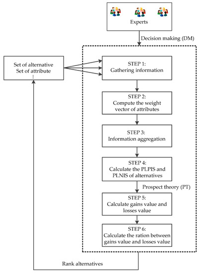
Under Definition 11, a novel MAGDM algorithm based on PT diagram is shown as follows. See Figure 1.

The specific steps of the algorithm are as follows.

Step 1. Information gathering process: individual reference points (RPs) over the alternatives on different attributes provided by experts are gathered as $\mathrm{R}={\left[{\mathrm{L}}_{\mathrm{ij}}(\mathrm{P})\right]}_{\mathrm{m}\times \mathrm{n}}$ by Equation (9).

Inspired by Reference [45], the extended cross-entry method is proposed to calculate the attributes’ weights.

Step 2. Compute the weight vector $\mathrm{w}={({\mathrm{w}}_1,{\mathrm{w}}_2,\dots ,{\mathrm{w}}_{\mathrm{n}})}^{\mathrm{T}}$ of $\mathrm{n}$ attributes $\mathrm{X}={({\mathrm{x}}_1,{\mathrm{x}}_2,\dots ,{\mathrm{x}}_{\mathrm{n}})}^{\mathrm{T}}$ as follows. See Equation (12).

$$\begin{array}{c}{E}_j=\frac{1}{m}{{\displaystyle \sum }}_{i=1}^m(1-\frac{2}{L_{j}T}{{\displaystyle \sum }}_{i=1}^{L_j}(((1+{qr}_{ij}^{(k_{ij})})ln(1+{qr}_{ij}^{(k_{ij})})+(1+q(1-\\ r_{(L_j-i+1)j}^{(k_{ij})})))Ln(1+q(1-r_{(L_j-i+1)j}^{(k_{ij})})))/2-((2+{qr}_{ij}^{(k_{ij})}+q(1-r_{(L_j-i+1)j}^{(k_{ij})}))/\\ 2)ln((2+{qr}_{ij}^{(k_{ij})}+q(1-r_{(L_j-i+1)j}^{(k_{ij})}))/2))),\\ w_j=\frac{1-E_j}{n-{{\displaystyle \sum }}_{j=1}^n{E}_j},i=1,2,\dots ,m,j=1,2,\dots ,n,L_j=\#L_{ij}(P)\end{array}$$

(12)

where $T=(1+q)ln(1+q)-(2+q)(ln(2+q)-ln2),q>0,$ $x_j$ is the $j$th attribute of the alternatives, $0\le w_j\le 1,$ and ${{\displaystyle \sum }}_{j=1}^n{w}_j=1$. In this paper, let $q=2$ [46].

Step 3. Aggregation process: get weighted DM matrix $R^{*}$. See Equation (13).

$$R^{*}={\left[L_{ij}^{*}(P)\right]}_{m\times n}=\left[\begin{array}{cccc}{L}_{11}^{*}(P)& L_{12}^{*}(P)& \cdots & L_{1n}^{*}(P)\\ L_{21}^{*}(P)& L_{22}^{*}(P)& \cdots & L_{2n}^{*}(P)\\ ⋮& ⋮& \ddots & ⋮\\ L_{m1}^{*}(P)& L_{m2}^{*}(P)& \cdots & L_{mn}^{*}(P)\end{array}\right]$$

(13)

where $L_{mn}^{*}(P)=(\frac{r_{ij}^{(k_{ij})}(L_{ij}^{(k_{ij})})}{g_i}\times P_{ij}^{(k_{ij})})\times w_j$, $i=1,2,\dots ,m,j=1,2,\dots ,n.$

Step 4. Calculate the positive ideal solution and the negative ideal solution respectively.

Then, the definitions of the probabilistic linguistic positive ideal solution (PLPIS) $L^{+}$ and the probabilistic linguistic negative ideal solution (PLNIS) $L^{-}$ are defined respectively as follows.

The PLPIS of the alternatives is

$$L^{+}=(L_1{(P)}^{+},L_2{(P)}^{+},\dots ,L_n{(P)}^{+}),$$

(14)

where $L_j{(P)}^{+}=L_{\Delta },\Delta =ma{x}_{i,j,k}\left\{\frac{r_{ij}^{(k_{ij})}(L_{ij}^{(k_{ij})})}{g_i}\times P_{ij}^{(k_{ij})}\right\}$.

The PLNIS of the alternatives is

$$L^{-}=(L_1{(P)}^{-},L_2{(P)}^{-},\dots ,L_n{(P)}^{-}),$$

(15)

where $L_j{(P)}^{-}=L_{\nabla },\nabla =mi{n}_{i,j,k}\left\{\frac{r_{ij}^{(k_{ij})}(L_{ij}^{(k_{ij})})}{g_i}\times P_{ij}^{(k_{ij})}\right\}$.

In order to select a preferred alternative or to rank all the alternatives, we should compute the distance between $A_i$ and $L^{+}$ and the distance between $A_i$ and $L^{-}$. Certainly, a better $A_i$ should be closer to $L^{+}$ and also farther from $L^{-}$.

Step 5. Calculate the gains value and the losses value: gains and losses are calculated with respect to the group reference points of the different alternatives.

Then, the prospect value is

$$V^{-}(d(L_{ij},L_j^{+}))=-\theta {(d(L_{ij},L_j^{+}))}^{\beta }.$$

(16)

$$V^{+}(d(L_{ij},L_j^{-}))={(d(L_{ij},L_j^{-}))}^{\alpha }.$$

(17)

where $\theta =$ 2.25, $\alpha =$ 0.88, and $\beta =$ 0.88 [47].

Step 6. Calculate the ration between the gains value and the losses value of each alternative.

$$C_i=\frac{\left|{{\displaystyle \sum }}_{j=1}^n{V}^{+}(d(L_{ij},L_j^{-}))\right|}{\left|{{\displaystyle \sum }}_{j=1}^n{V}^{-}(d(L_{ij},L_j^{+}))\right|},i=1,2,\dots ,m,j=1,2,\dots ,n.$$

(18)

Rank the alternatives by the values $C_i$ of $A_i$. Certainly, the bigger the closeness degree is, the better the alternative is.

4. Case Studies

With the popularity of the Internet, e-commerce has become an indispensable field in daily life. For example, if people want to purchase a car, they will be concerned with all kinds of information about cars on the Internet. People take all kinds of information into consideration to decide which car to buy, such as scoring data, word-of-mouth data, forum reviews, and so on. For example, there are seven new energy cars to choose. People collect assessment information of these cars from users by the three ways (scoring data, word-of-mouth data, and forum reviews) on eight attributes, which are space, power, manipulate, power consumption, comfort, appearance, interior decoration, and cost performance on the “Auto Home” website. Note them as $x_1,x_2,x_3,x_4,x_5,x_6,x_7,$ and $x_8$ respectively. The seven cars are ZhiXuan ($A_1$), WeiChiFS ($A_2$), LiWei ($A_3$), FeiDu ($A_4$), RuiNa RV ($A_5$), KiaK2 ($A_6$), and JinRui ($A_7$) respectively. Since scoring data online is a 5-point system, the scoring data to assessment information is operated to 5-granular linguistic term sets. The word-of-mouth data of the overall assessment for cars can be mapped to 7-granular linguistic term sets. Due to the complexity of the community review information, this information can be operated to 9-granular linguistic term sets.

4.1. The Applications of the Algorithm

The applications of the algorithm based on PT are shown as follows.

Step 1. Collect the users’ assessment information on the “Auto Home” website until May 20 in 2018. See

Table 1. The assessment information from scoring data by $S_5$.

Alternative	${\mathit{x}}_1$	${\mathit{x}}_2$	${\mathit{x}}_3$	${\mathit{x}}_4$	${\mathit{x}}_5$	${\mathit{x}}_6$	${\mathit{x}}_7$	${\mathit{x}}_8$
$A_1$	$S_5^5$	$S_5^5$	$S_5^5$	$S_4^5$	$S_5^5$	$S_5^5$	$S_4^5$	$S_5^5$
$A_2$	$S_{4.79}^5$	$S_{4.76}^5$	$S_{4.78}^5$	$S_{4.93}^5$	$S_{4.45}^5$	$S_{4.87}^5$	$S_{4.15}^5$	$S_{4.88}^5$
$A_3$	$S_{4.59}^5$	$S_{4.33}^5$	$S_{4.39}^5$	$S_{4.90}^5$	$S_{4.04}^5$	$S_{4.34}^5$	$S_{3.68}^5$	$S_{4.35}^5$
$A_4$	$S_{4.83}^5$	$S_{4.89}^5$	$S_{4.13}^5$	$S_{4.79}^5$	$S_{3.41}^5$	$S_{4.64}^5$	$S_{3.56}^5$	$S_{4.42}^5$
$A_5$	$S_{4.60}^5$	$S_{4.04}^5$	$S_{4.06}^5$	$S_{4.15}^5$	$S_{3.68}^5$	$S_{4.85}^5$	$S_{3.79}^5$	$S_{4.49}^5$
$A_6$	$S_{4.25}^5$	$S_{3.80}^5$	$S_{4.38}^5$	$S_{4.37}^5$	$S_{3.63}^5$	$S_{4.63}^5$	$S_{4.05}^5$	$S_{4.44}^5$
$A_7$	$S_{3.55}^5$	$S_{3.60}^5$	$S_{4.38}^5$	$S_{4.28}^5$	$S_{3.53}^5$	$S_{4.62}^5$	$S_{3.34}^5$	$S_{4.40}^5$

,

Table 2. The assessment information from word-of-mouth data by $S_7$.

Alternative	${\mathit{x}}_1$	${\mathit{x}}_2$	${\mathit{x}}_3$	${\mathit{x}}_4$	${\mathit{x}}_5$	${\mathit{x}}_6$	${\mathit{x}}_7$	${\mathit{x}}_8$
$A_1$	$S_6^7$	$S_3^7$	$-$	$S_5^7$	$S_2^7$	$S_7^7$	$S_2^7$	$S_4^7$
$A_2$	$S_6^7$	$S_3^7$	$S_7^7$	$S_5^7$	$S_4^7$	$S_7^7$	$S_2^7$	$S_5^7$
$A_3$	$S_5^7$	$S_3^7$	$-$	$S_5^7$	$S_4^7$	$S_6^7$	$S_4^7$	$S_6^7$
$A_4$	$S_7^7$	$S_3^7$	$S_5^7$	$S_5^7$	$S_2^7$	$S_7^7$	$-$	$S_5^7$
$A_5$	$S_5^7$	$S_4^7$	$S_6^7$	$S_5^7$	$S_3^7$	$S_7^7$	$S_2^7$	$S_6^7$
$A_6$	$S_6^7$	$S_3^7$	$S_7^7$	$S_6^7$	$S_5^7$	$S_6^7$	$S_3^7$	$S_4^7$
$A_7$	$S_5^7$	$S_5^7$	$S_4^7$	$-$	$S_3^7$	$S_5^7$	$S_3^7$	$S_5^7$

and

Table 3. The assessment information from forum reviews data by $S_9$.

Alternative	${\mathit{x}}_1$	${\mathit{x}}_2$	${\mathit{x}}_3$	${\mathit{x}}_4$	${\mathit{x}}_5$	${\mathit{x}}_6$	${\mathit{x}}_7$	${\mathit{x}}_8$
$A_1$	$S_8^9$	$S_6^9$	$S_7^9$	$S_8^9$	$S_4^9$	$S_8^9$	$S_7^9$	$S_7^9$
$A_2$	$S_7^9$	$S_7^9$	$S_7^9$	$S_8^9$	$S_6^9$	$S_7^9$	$S_6^9$	$S_9^9$
$A_3$	$S_9^9$	$S_6^9$	$S_9^9$	$S_8^9$	$S_4^9$	$S_4^9$	$S_1^9$	$S_7^9$
$A_4$	$S_9^9$	$S_4^9$	$S_4^9$	$S_9^9$	$S_3^9$	$S_6^9$	$S_1^9$	$S_6^9$
$A_5$	$S_8^9$	$S_5^9$	$S_3^9$	$S_3^9$	$S_4^9$	$S_7^9$	$S_4^9$	$S_7^9$
$A_6$	$S_4^9$	$S_6^9$	$S_9^9$	$S_9^9$	$S_2^9$	$S_8^9$	$S_4^9$	$S_8^9$
$A_7$	$S_6^9$	$S_5^9$	$S_8^9$	$S_5^9$	$S_6^9$	$S_8^9$	$S_8^9$	$S_9^9$

.

Here, the scoring data (see Table 1) are the final average values of the seven cars on eight attributes from the scoring data. The assessment information (see Table 2) is the general impression from the word-of-mouth data. The assessment information (see Table 3) is from forum reviews data. These data are obtained on the “Auto Home” website.

Then, we get the users’ overall assessment probabilistic linguistic term sets. See

Table 4. The assessment probabilistic linguistic assessment matrix.

Alternative	${\mathit{x}}_1$	${\mathit{x}}_2$	${\mathit{x}}_3$	${\mathit{x}}_4$
$A_1$	$\left\{S_5^5(\frac{1}{3}),S_6^7(\frac{1}{3}),S_8^9(\frac{1}{3})\right\}$	$\left\{S_1^5(\frac{1}{3}),S_3^7(\frac{1}{3}),S_6^9(\frac{1}{3})\right\}$	$\left\{S_5^5(\frac{1}{2}),S_7^9(\frac{1}{2})\right\}$	$\left\{S_4^5(\frac{1}{3}),S_5^7(\frac{1}{3}),S_8^9(\frac{1}{3})\right\}$
$A_2$	$\left\{S_{4.79}^5(\frac{1}{3}),S_6^7(\frac{1}{3}),S_7^9(\frac{1}{3})\right\}$	$\left\{S_{4.76}^5(\frac{1}{3}),S_3^7(\frac{1}{3}),S_7^9(\frac{1}{3})\right\}$	$\left\{S_{4.78}^5(\frac{1}{3}),S_7^7(\frac{1}{3}),S_7^9(\frac{1}{3})\right\}$	$\left\{S_{4.93}^5(\frac{1}{3}),S_5^7(\frac{1}{3}),S_8^9(\frac{1}{3})\right\}$
$A_3$	$\left\{S_{4.59}^5(\frac{1}{3}),S_5^7(\frac{1}{3}),S_9^9(\frac{1}{3})\right\}$	$\left\{S_{4.33}^5(\frac{1}{3}),S_3^7(\frac{1}{3}),S_6^9(\frac{1}{3})\right\}$	$\left\{S_{4.39}^5(\frac{1}{2}),S_9^9(\frac{1}{2})\right\}$	$\left\{S_{4.90}^5(\frac{1}{3}),S_5^7(\frac{1}{3}),S_8^9(\frac{1}{3})\right\}$
$A_4$	$\left\{S_{4.83}^5(\frac{1}{3}),S_7^7(\frac{1}{3}),S_9^9(\frac{1}{3})\right\}$	$\left\{S_{4.89}^5(\frac{1}{3}),S_3^7(\frac{1}{3}),S_4^9(\frac{1}{3})\right\}$	$\left\{S_{4.13}^5(\frac{1}{3}),S_5^7(\frac{1}{3}),S_4^9(\frac{1}{3})\right\}$	$\left\{S_{4.79}^5(\frac{1}{3}),S_5^7(\frac{1}{3}),S_9^9(\frac{1}{3})\right\}$
$A_5$	$\left\{S_{4.60}^5(\frac{1}{3}),S_5^7(\frac{1}{3}),S_8^9(\frac{1}{3})\right\}$	$\left\{S_{4.04}^5(\frac{1}{3}),S_4^7(\frac{1}{3}),S_5^9(\frac{1}{3})\right\}$	$\left\{S_{4.06}^5(\frac{1}{3}),S_6^7(\frac{1}{3}),S_3^9(\frac{1}{3})\right\}$	$\left\{S_{4.15}^5(\frac{1}{3}),S_5^7(\frac{1}{3}),S_3^9(\frac{1}{3})\right\}$
$A_6$	$\left\{S_{4.25}^5(\frac{1}{3}),S_6^7(\frac{1}{3}),S_4^9(\frac{1}{3})\right\}$	$\left\{S_{3.80}^5(\frac{1}{3}),S_3^7(\frac{1}{3}),S_6^9(\frac{1}{3})\right\}$	$\left\{S_{4.38}^5(\frac{1}{3}),S_7^7(\frac{1}{3}),S_9^9(\frac{1}{3})\right\}$	$\left\{S_{4.37}^5(\frac{1}{3}),S_6^7(\frac{1}{3}),S_9^9(\frac{1}{3})\right\}$
$A_7$	$\left\{S_{3.55}^5(\frac{1}{3}),S_5^7(\frac{1}{3}),S_6^9(\frac{1}{3})\right\}$	$\left\{S_{3.60}^5(\frac{1}{3}),S_5^7(\frac{1}{3}),S_5^9(\frac{1}{3})\right\}$	$\left\{S_{4.38}^5(\frac{1}{3}),S_4^7(\frac{1}{3}),S_8^9(\frac{1}{3})\right\}$	$\left\{S_{4.28}^5(\frac{1}{2}),S_5^9(\frac{1}{2})\right\}$
Alternative	${\mathit{x}}_5$	${\mathit{x}}_6$	${\mathit{x}}_7$	${\mathit{x}}_8$
$A_1$	$\left\{S_5^5(\frac{1}{3}),S_2^7(\frac{1}{3}),S_4^9(\frac{1}{3})\right\}$	$\left\{S_5^5(\frac{1}{3}),S_7^7(\frac{1}{3}),S_8^9(\frac{1}{3})\right\}$	$\left\{S_4^5(\frac{1}{3}),S_2^7(\frac{1}{3}),S_7^9(\frac{1}{3})\right\}$	$\left\{S_5^5(\frac{1}{3}),S_4^7(\frac{1}{3}),S_7^9(\frac{1}{3})\right\}$
$A_2$	$\left\{S_{4.45}^5(\frac{1}{3}),S_4^7(\frac{1}{3}),S_6^9(\frac{1}{3})\right\}$	$\left\{S_{4.87}^5(\frac{1}{3}),S_7^7(\frac{1}{3}),S_7^9(\frac{1}{3})\right\}$.	$\left\{S_{4.15}^5(\frac{1}{3}),S_2^7(\frac{1}{3}),S_6^9(\frac{1}{3})\right\}$	$\left\{S_{4.88}^5(\frac{1}{3}),S_5^7(\frac{1}{3}),S_9^9(\frac{1}{3})\right\}$
$A_3$	$\left\{S_{4.04}^5(\frac{1}{3}),S_4^7(\frac{1}{3}),S_4^9(\frac{1}{3})\right\}$	$\left\{S_{4.34}^5(\frac{1}{3}),S_6^7(\frac{1}{3}),S_4^9(\frac{1}{3})\right\}$	$\left\{S_{3.68}^5(\frac{1}{3}),S_4^7(\frac{1}{3}),S_1^9(\frac{1}{3})\right\}$	$\left\{S_{4.35}^5(\frac{1}{3}),S_6^7(\frac{1}{3}),S_7^9(\frac{1}{3})\right\}$
$A_4$	$\left\{S_{3.41}^5(\frac{1}{3}),S_2^7(\frac{1}{3}),S_3^9(\frac{1}{3})\right\}$	$\left\{S_{4.64}^5(\frac{1}{3}),S_7^7(\frac{1}{3}),S_6^9(\frac{1}{3})\right\}$	$\left\{S_{3.56}^5(\frac{1}{2}),S_1^9(\frac{1}{2})\right\}$	$\left\{S_{4.42}^5(\frac{1}{3}),S_5^7(\frac{1}{3}),S_6^9(\frac{1}{3})\right\}$
$A_5$	$\left\{S_{3.68}^5(\frac{1}{3}),S_3^7(\frac{1}{3}),S_4^9(\frac{1}{3})\right\}$	$\left\{S_{4.85}^5(\frac{1}{3}),S_7^7(\frac{1}{3}),S_7^9(\frac{1}{3})\right\}$	$\left\{S_{3.79}^5(\frac{1}{3}),S_2^7(\frac{1}{3}),S_4^9(\frac{1}{3})\right\}$	$\left\{S_{4.49}^5(\frac{1}{3}),S_6^7(\frac{1}{3}),S_7^9(\frac{1}{3})\right\}$
$A_6$	$\left\{S_{3.63}^5(\frac{1}{3}),S_5^7(\frac{1}{3}),S_2^9(\frac{1}{3})\right\}$	$\left\{S_{4.63}^5(\frac{1}{3}),S_6^7(\frac{1}{3}),S_8^9(\frac{1}{3})\right\}$	$\left\{S_{4.05}^5(\frac{1}{3}),S_3^7(\frac{1}{3}),S_4^9(\frac{1}{3})\right\}$	$\left\{S_{4.44}^5(\frac{1}{3}),S_4^7(\frac{1}{3}),S_8^9(\frac{1}{3})\right\}$
$A_7$	$\left\{S_{3.53}^5(\frac{1}{3}),S_3^7(\frac{1}{3}),S_6^9(\frac{1}{3})\right\}$	$\left\{S_{4.62}^5(\frac{1}{3}),S_5^7(\frac{1}{3}),S_8^9(\frac{1}{3})\right\}$	$\left\{S_{3.34}^5(\frac{1}{3}),S_3^7(\frac{1}{3}),S_8^9(\frac{1}{3})\right\}$	$\left\{S_{4.40}^5(\frac{1}{3}),S_5^7(\frac{1}{3}),S_9^9(\frac{1}{3})\right\}$

.

Then, we get the normalized DM matrix by Definition 5. See

Table 5. The normalized decision-making (DM) matrix.

Alternative	${\mathit{x}}_1$	${\mathit{x}}_2$	${\mathit{x}}_3$	${\mathit{x}}_4$
$A_1$	$\left\{S_{\frac{1}{3}},S_{\frac{8}{27}},S_{\frac{2}{7}}\right\}$	$\left\{S_{\frac{1}{3}},S_{\frac{2}{9}},S_{\frac{1}{7}}\right\}$	$\left\{S_{\frac{1}{2}},S_{\frac{7}{18}},S_0\right\}$	$\left\{S_{\frac{8}{27}},S_{\frac{4}{15}},S_{\frac{5}{21}}\right\}$
$A_2$	$\left\{S_{\frac{4.79}{15}},S_{\frac{2}{7}},S_{\frac{7}{27}}\right\}$	$\left\{S_{\frac{4.76}{15}},S_{\frac{7}{27}},S_{\frac{1}{7}}\right\}$	$\left\{S_{\frac{1}{3}},S_{\frac{4.78}{15}},S_{\frac{7}{27}}\right\}$	$\left\{S_{\frac{4.93}{15}},S_{\frac{8}{27}},S_{\frac{5}{21}}\right\}$
$A_3$	$\left\{S_{\frac{1}{3}},S_{\frac{4.59}{15}},S_{\frac{5}{21}}\right\}$	$\left\{S_{\frac{4.33}{15}},S_{\frac{2}{9}},S_{\frac{1}{7}}\right\}$	$\left\{S_{\frac{1}{2}},S_{\frac{4.39}{10}},S_0\right\}$	$\left\{S_{\frac{4.90}{15}},S_{\frac{8}{27}},S_{\frac{5}{21}}\right\}$
$A_4$	$\left\{S_{\frac{2}{3}},S_{\frac{4.83}{15}},S_0\right\}$	$\left\{S_{\frac{4.89}{15}},S_{\frac{4}{27}},S_{\frac{1}{7}}\right\}$	$\left\{S_{\frac{4.13}{15}},S_{\frac{5}{21}},S_{\frac{4}{27}}\right\}$	$\left\{S_{\frac{1}{3}},S_{\frac{4.79}{15}},S_{\frac{5}{21}}\right\}$
$A_5$	$\left\{S_{\frac{4.60}{15}},S_{\frac{8}{27}},S_{\frac{5}{21}}\right\}$	$\left\{S_{\frac{4.04}{15}},S_{\frac{4}{21}},S_{\frac{5}{27}}\right\}$	$\left\{S_{\frac{2}{7}},S_{\frac{4.06}{15}},S_{\frac{1}{9}}\right\}$	$\left\{S_{\frac{4.15}{15}},S_{\frac{5}{21}},S_{\frac{1}{9}}\right\}$
$A_6$	$\left\{S_{\frac{2}{7}},S_{\frac{4.25}{15}},S_{\frac{4}{27}}\right\}$	$\left\{S_{\frac{3.80}{15}},S_{\frac{2}{9}},S_{\frac{1}{7}}\right\}$	$\left\{S_{\frac{2}{3}},S_{\frac{4.38}{15}},S_0\right\}$	$\left\{S_{\frac{1}{3}},S_{\frac{4.37}{15}},S_{\frac{2}{7}}\right\}$
$A_7$	$\left\{S_{\frac{5}{21}},S_{\frac{3.55}{15}},S_{\frac{2}{9}}\right\}$	$\left\{S_{\frac{3.60}{15}},S_{\frac{5}{21}},S_{\frac{5}{27}}\right\}$	$\left\{S_{\frac{8}{27}},S_{\frac{4.38}{15}},S_{\frac{4}{21}}\right\}$	$\left\{S_{\frac{4.28}{10}},S_{\frac{5}{18}},S_0\right\}$
Alternative	${\mathit{x}}_5$	${\mathit{x}}_6$	${\mathit{x}}_7$	${\mathit{x}}_8$
$A_1$	$\left\{S_{\frac{1}{3}},S_{\frac{4}{27}},S_{\frac{2}{21}}\right\}$	$\left\{S_{\frac{2}{3}},S_{\frac{8}{27}},S_0\right\}$	$\left\{S_{\frac{4}{15}},S_{\frac{7}{27}},S_{\frac{2}{21}}\right\}$	$\left\{S_{\frac{1}{3}},S_{\frac{7}{27}},S_{\frac{4}{21}}\right\}$
$A_2$	$\left\{S_{\frac{4.45}{15}},S_{\frac{2}{9}},S_{\frac{4}{21}}\right\}$	$\left\{S_{\frac{1}{3}},S_{\frac{4.87}{15}},S_{\frac{7}{27}}\right\}$	$\left\{S_{\frac{4.15}{15}},S_{\frac{2}{9}},S_{\frac{2}{21}}\right\}$	$\left\{S_{\frac{1}{3}},S_{\frac{4.88}{15}},S_{\frac{5}{21}}\right\}$
$A_3$	$\left\{S_{\frac{4.04}{15}},S_{\frac{4}{21}},S_{\frac{4}{27}}\right\}$	$\left\{S_{\frac{4.34}{15}},S_{\frac{2}{7}},S_{\frac{4}{27}}\right\}$	$\left\{S_{\frac{3.68}{15}},S_{\frac{4}{21}},S_{\frac{1}{27}}\right\}$	$\left\{S_{\frac{4.35}{15}},S_{\frac{2}{7}},S_{\frac{7}{27}}\right\}$
$A_4$	$\left\{S_{\frac{3.41}{15}},S_{\frac{1}{9}},S_{\frac{2}{21}}\right\}$	$\left\{S_{\frac{1}{3}},S_{\frac{4.64}{15}},S_{\frac{2}{9}}\right\}$	$\left\{S_{\frac{3.56}{10}},S_{\frac{1}{18}},S_0\right\}$	$\left\{S_{\frac{4.42}{15}},S_{\frac{5}{21}},S_{\frac{2}{9}}\right\}$
$A_5$	$\left\{S_{\frac{3.68}{15}},S_{\frac{4}{27}},S_{\frac{1}{7}}\right\}$	$\left\{S_{\frac{1}{3}},S_{\frac{4.85}{15}},S_{\frac{7}{27}}\right\}$	$\left\{S_{\frac{3.79}{15}},S_{\frac{4}{27}},S_{\frac{2}{21}}\right\}$	$\left\{S_{\frac{4.49}{15}},S_{\frac{2}{7}},S_{\frac{7}{27}}\right\}$
$A_6$	$\left\{S_{\frac{3.63}{15}},S_{\frac{5}{21}},S_{\frac{2}{27}}\right\}$	$\left\{S_{\frac{4.63}{15}},S_{\frac{8}{27}},S_{\frac{2}{7}}\right\}$	$\left\{S_{\frac{4.05}{15}},S_{\frac{4}{27}},S_{\frac{1}{7}}\right\}$	$\left\{S_{\frac{8}{27}},S_{\frac{4.44}{15}},S_{\frac{4}{21}}\right\}$
$A_7$	$\left\{S_{\frac{3.53}{15}},S_{\frac{2}{9}},S_{\frac{1}{7}}\right\}$	$\left\{S_{\frac{4.62}{15}},S_{\frac{8}{27}},S_{\frac{5}{21}}\right\}$	$\left\{S_{\frac{8}{27}},S_{\frac{3.34}{15}},S_{\frac{1}{7}}\right\}$.	$\left\{S_{\frac{1}{3}},S_{\frac{4.40}{15}},S_{\frac{5}{21}}\right\}$

.

Here, $S_{{\alpha }_i}$ is defined as follows: ${\alpha }_i=\frac{r_{ij}^{(k_{ij})}(L_{ij}^{(k_{ij})})}{g_i}\times P_{ij}^{(k_{ij})},i=1,2,\dots ,m,j=1,2,\dots ,n.$ For example, ${\alpha }_i=\frac{4.71}{5}\times \frac{1}{3}=\frac{4.71}{15}$.

Step 2. Calculate the weight vector $w={(w_1,w_2,w_3,w_4,w_5,w_6,w_7,w_8)}^T$ on the eight attributes $X={(x_1,x_2,x_3,x_4,x_5,x_6,x_7,x_8)}^T$ by Equation (12). See

Table 6. The weights of the attributes.

Attribute	$x_1$	$x_2$	$x_3$	$x_4$	$x_5$	$x_6$	$x_7$	$x_8$
Weight	0.0922	0.1481	0.1022	0.1023	0.1815	0.0832	0.1948	0.0955

.

Step 3. Get a weighted DM matrix. See

Table 7. The weighted normalized DM matrix.

Alternative	${\mathit{x}}_1$	${\mathit{x}}_2$	${\mathit{x}}_3$	${\mathit{x}}_4$
$A_1$	(0.0307,0.0273,0.0263)	(0.0494,0.0329,0.0212)	(0.0511,0.0397,0.0000)	(0.0303,0.0273,0.0244)
$A_2$	(0.0294,0.0263,0.0239)	(0.0470,0.0384,0.0212)	(0.0341,0.0326,0.0265)	(0.0336,0.0303,0.0244)
$A_3$	(0.0307,0.0282,0.0220)	(0.0428,0.0329,0.0212)	(0.0511,0.0449,0.0000)	(0.0334,0.0303,0.0244)
$A_4$	(0.0615,0.0297,0.0000)	(0.0483,0.0219,0.0212)	(0.0281,0.0243,0.0151)	(0.0341,0.0327,0.0244)
$A_5$	(0.0283,0.0273,0.0220)	(0.0399,0.0282,0.0274)	(0.0292,0.0277,0.0114)	(0.0283,0.0244,0.0114)
$A_6$	(0.0263,0.0261,0.0137)	(0.0375,0.0329,0.0212)	(0.0681,0.0298,0.0000)	(0.0341,0.0298,0.0292)
$A_7$	(0.0220,0.0218,0.0205)	(0.0355,0.0353,0.0274)	(0.0303,0.0298,0.0195)	(0.0438,0.0284,0.0000)
Alternative	${\mathit{x}}_5$	${\mathit{x}}_6$	${\mathit{x}}_7$	${\mathit{x}}_8$
$A_1$	(0.0605,0.0269,0.0173)	(0.0555,0.0247,0.0000)	(0.0519,0.0505,0.0186)	(0.0318,0.0248,0.0182)
$A_2$	(0.0538,0.0403,0.0346)	(0.0277,0.0270,0.0216)	(0.0539,0.0433,0.0186)	(0.0318,0.0311,0.0227)
$A_3$	(0.0489,0.0346,0.0269)	(0.0241,0.0238,0.0123)	(0.0478,0.0371,0.0072)	(0.0277,0.0273,0.0248)
$A_4$	(0.0413,0.0202,0.0173)	(0.0277,0.0257,0.0185)	(0.0693,0.0108,0.0000)	(0.0281,0.0227,0.0212)
$A_5$	(0.0445,0.0269,0.0259)	(0.0277,0.0269,0.0216)	(0.0492,0.0289,0.0186)	(0.0286,0.0273,0.0248)
$A_6$	(0.0439,0.0432,0.0134)	(0.0257,0.0247,0.0238)	(0.0526,0.0289,0.0278)	(0.0283,0.0283,0.0182)
$A_7$	(0.0427,0.0403,0.0259)	(0.0256,0.0247,0.0198)	(0.0577,0.0434,0.0278)	(0.0318,0.0280,0.0227)

.

Here, in order to calculate conveniently, we only note ${\alpha }_i$ instead of $S_{{\alpha }_i}$.

Step 4. Calculate the PLPIS and PLNIS respectively.

The normalized PLPIS is as follows (see

Table 8. The positive ideal solution.

Attribute	${\mathit{x}}_1$	${\mathit{x}}_2$	${\mathit{x}}_3$	${\mathit{x}}_4$
PLPIS	(0.0615,0.0297,0.0263)	(0.0494,0.0384,0.0274)	(0.0681,0.0449,0.0265)	(0.0438,0.0327,0.0292)
Attribute	${\mathit{x}}_5$	${\mathit{x}}_6$	${\mathit{x}}_7$	${\mathit{x}}_8$
PLPIS	(0.0605,0.0432,0.0346)	(0.0555,0.0270,0.0238)	(0.0693,0.0505,0.0278)	(0.0318,0.0311,0.0248)

):

The normalized PLNIS is as follows (see

Table 9. The negative ideal solution.

Attribute	${\mathit{x}}_1$	${\mathit{x}}_2$	${\mathit{x}}_3$	${\mathit{x}}_4$
PLNIS	(0.0220,0.0218,0.0000)	(0.0355,0.0219,0.0212)	(0.0281,0.0243,0.0000)	(0.0283,0.0244,0.0000)
Attribute	${\mathit{x}}_5$	${\mathit{x}}_6$	${\mathit{x}}_7$	${\mathit{x}}_8$
PLNIS	(0.0413,0.0202,0.0134)	(0.0241,0.0238,0.0000)	(0.0478,0.0108,0.0000)	(0.0277,0.0227,0.0182)

):

Step 5. The results of $V(A_i,L^{-})$ and $V(A_i,L^{+})(i=1,2,\dots ,7)$ are as follows. See

Table 10. The results of $V(A_i,L^{-})$.

	Attribute	${\mathit{A}}_1$	${\mathit{A}}_2$	${\mathit{A}}_3$	${\mathit{A}}_4$	${\mathit{A}}_5$	${\mathit{A}}_6$	${\mathit{A}}_7$
Distance Parameter
$\lambda =1$		2.2775	2.3581	2.1791	2.0516	2.0394	2.1872	2.1285
$\lambda =2$		2.4984	2.3883	2.2884	2.2535	2.0766	2.3228	2.2020

and

Table 11. The results of $V(A_i,L^{+})$.

	Attribute	${\mathit{A}}_1$	${\mathit{A}}_2$	${\mathit{A}}_3$	${\mathit{A}}_4$	${\mathit{A}}_5$	${\mathit{A}}_6$	${\mathit{A}}_7$
Distance Parameter
$\lambda =1$		4.8225	4.9277	4.5605	4.3157	4.2010	4.5976	4.4524
$\lambda =2$		5.2726	5.0031	4.7956	4.7448	4.3088	4.8694	4.5975

.

Step 6. Calculate the closeness coefficient $C_i$ of $A_i(i=1,2,\dots ,7)$ by Equation (18). The results are as follows. See

Table 12. The ration $C_i$ of $A_i$.

	Attribute	${\mathit{A}}_1$	${\mathit{A}}_2$	${\mathit{A}}_3$	${\mathit{A}}_4$	${\mathit{A}}_5$	${\mathit{A}}_6$	${\mathit{A}}_7$
Distance Parameter
$\lambda =1$		0.4723	0.4785	0.4778	0.4754	0.4854	0.4776	0.4781
$\lambda =2$		0.4739	0.4774	0.4772	0.4779	0.4820	0.4770	0.4789

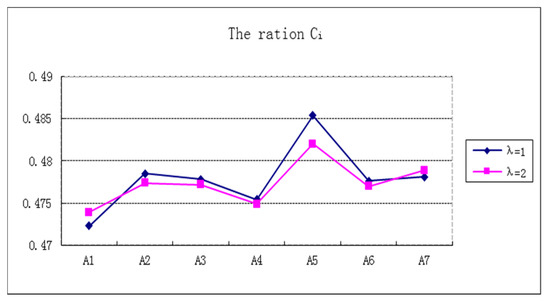
and Figure 2.

Rank the alternatives by the values $C_i$ of $A_i(i=1,2,\dots ,7)$. See

Table 13. The ranking of $A_i$.

Distance Parameter	Rank
$\lambda =1$	$A_5\succ A_2\succ A_7\succ A_3\succ A_6\succ A_4\succ A_1$
$\lambda =2$	$A_5\succ A_7\succ A_2\succ A_3\succ A_6\succ A_4\succ A_1$

.

4.2. Sensitivity Analysis

In order to analyze the sensitivity of the parameters, take the different parameters [38] and rank $A_i(i=1,2,\dots ,7)$ by the algorithm based on PT as in Section 4.1. Then, the results are as follows.

Calculate the closeness coefficient $C_i$ of each alternative $A_i(i=1,2,\dots ,7)$by Equation (18). See

Table 14. The ration $C_i$ of $A_i$.

Distance Parameter	Parameters			${\mathit{A}}_1$	${\mathit{A}}_2$	${\mathit{A}}_3$	${\mathit{A}}_4$	${\mathit{A}}_5$	${\mathit{A}}_6$	${\mathit{A}}_7$
$\lambda =1$	$\alpha =0.85,$	$\beta =0.85$	$\theta =4.1$	0.2587	0.2620	0.2616	0.2604	0.2657	0.2615	0.2617
	$\alpha =0.725$	$\beta =0.717$	$\theta =2.04$	0.5097	0.5152	0.5146	0.5123	0.5210	0.5143	0.5142
	$\alpha =0.89$	$\beta =0.92$	$\theta =2.25$	0.4939	0.5003	0.5005	0.4985	0.5101	0.5003	0.5016
Distance Parameter	Parameters			${\mathit{A}}_1$	${\mathit{A}}_2$	${\mathit{A}}_3$	${\mathit{A}}_4$	${\mathit{A}}_5$	${\mathit{A}}_6$	${\mathit{A}}_7$
$\lambda =2$	$\alpha =0.85$	$\beta =0.85$	$\theta =4.1$	0.2595	0.2614	0.2613	0.2601	0.2638	0.2612	0.2622
	$\alpha =0.725$	$\beta =0.717$	$\theta =2.04$	0.5114	0.5141	0.5140	0.5121	0.5178	0.5139	0.5152
	$\alpha =0.89$	$\beta =0.92$	$\theta =2.25$	0.4939	0.4988	0.4991	0.4965	0.5060	0.4985	0.5019

.

Rank the alternatives by the values $C_i$ of $A_i(i=1,2,\dots ,7)$. See

Table 15. The ranking of $A_i$.

Distance Parameter	Parameters			Rank
$\lambda =1$	$\alpha =0.85,$	$\beta =0.85$	$\theta =4.1$	$A_5\succ A_2\succ A_7\succ A_3\succ A_6\succ A_4\succ A_1$
	$\alpha =0.725$	$\beta =0.717$	$\theta =2.04$	$A_5\succ A_2\succ A_3\succ A_6\succ A_7\succ A_4\succ A_1$
	$\alpha =0.89$	$\beta =0.92$	$\theta =2.25$	$A_5\succ A_7\succ A_3\succ A_2=A_6\succ A_4\succ A_1$
$\lambda =2$	$\alpha =0.85$	$\beta =0.85$	$\theta =4.1$	$A_5\succ A_7\succ A_2\succ A_3\succ A_6\succ A_4\succ A_1$
	$\alpha =0.725$	$\beta =0.717$	$\theta =2.04$	$A_5\succ A_7\succ A_2\succ A_3\succ A_6\succ A_4\succ A_1$
	$\alpha =0.89$	$\beta =0.92$	$\theta =2.25$	$A_5\succ A_7\succ A_3\succ A_2\succ A_6\succ A_4\succ A_1$

.

From Table 14 and Table 15, we can find the rankings of the alternatives $A_i(i=1,2,\dots ,7)$ are different but only when $\alpha =0.85$, $\beta =0.85$, and $\theta =4.1$ ($\lambda =2$) and $\alpha =0.725$, $\beta =0.717$, and $\theta =2.04(\lambda =2)$, respectively; the results are coincident by the algorithm based on PT. The ranking results are different as the parameters ($\theta ,\alpha ,\mathrm{and}\beta )$ are changed. This result is consistent with the meaning of the parameters ($\theta ,\alpha ,\mathrm{and}\beta )$. Here, $\alpha \mathrm{and}\beta$ are power parameters related to gains and losses, respectively. $\theta$ is the risk-aversion parameter, which has the characteristic of being steeper for losses than for gains when $\theta >1$: The larger the value, the greater the degree of risk. Then the ranking of $A_i$ is different. Therefore, the algorithm based on PT proposed in Section 4.1 is scientific.

4.3. Comparative Analysis

In order to illustrate the feasibility and efficiency of the algorithm-based PT, we calculate the other results by the other three algorithms based on TOPSIS, VIKOR, and Pang Qi et al.’s method respectively.

The results of the algorithm based on TOPSIS are as follows:

The closeness coefficient of $A_i(i=1,2,\dots ,7)$ is

$$C{D}_i=\frac{(1-\delta )d(A_i,L^{-})}{\delta d(A_i,L^{+})+(1-\delta )d(A_i,L^{-})}.$$

(19)

The parameter $\delta \in \left[0,1\right]$ represents the risk preferences of the decision maker. If $\delta >0.5,$ then it means that the DMs are optimistic. If $\delta <0.5$, then it means they are pessimistic. The value of $\delta$ should be given by DMs beforehand. Here, let $\delta =0.5$. The higher $C{D}_i$ is, the better the alternative is.

Calculate the closeness coefficient $C{D}_i$ by Equation (19), and the results are as follows. See

Table 16. The closeness coefficient $C{D}_i$.

	Attribute	${\mathit{A}}_1$	${\mathit{A}}_2$	${\mathit{A}}_3$	${\mathit{A}}_4$	${\mathit{A}}_5$	${\mathit{A}}_6$	${\mathit{A}}_7$
Distance Parameter
$\lambda =1$		0.5170	0.5209	0.5202	0.5187	0.5247	0.5201	0.5206
$\lambda =2$		0.5181	0.5202	0.5200	0.5186	0.5228	0.5199	0.5211

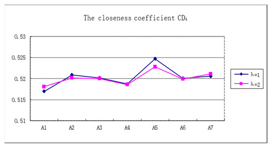
and Figure 3.

Rank the alternatives by the values $C{D}_i$ of $A_i$($i=1,2,\dots ,7$). See

Table 17. The ranking of $A_i$.

Distance Parameter	Rank
$\lambda =1$	$A_5\succ A_2\succ A_7\succ A_3\succ A_6\succ A_4\succ A_1$
$\lambda =2$	$A_5\succ A_7\succ A_2\succ A_3\succ A_6\succ A_4\succ A_1$

.

The results of the algorithm based on VIKOR are as follows:

The compromise index:

$$M{C}_i=v\frac{M{U}_i-M{U}^{+}}{M{U}^{-}-M{U}^{+}}+(1-v)\frac{M{R}_i-M{R}^{+}}{M{R}^{-}-M{R}^{+}},$$

(20)

The whole benefit index:

$$M{U}_i={{\displaystyle \sum }}_{j=1}^n{w}_j\frac{d(L_{ij}(P),L_j{(P)}^{+})}{d(L_j{(P)}^{+},L_j{(P)}^{-})},$$

(21)

The compromise index:

$$M{R}_i=\max \left[w_j\frac{d(L_{ij}(P),L_j{(P)}^{+})}{d(L_j{(P)}^{+},L_j{(P)}^{-})}\right],$$

(22)

where $M{U}^{+}=\max \left\{M{U}_i\right\},M{U}^{-}=\min \left\{M{U}_i\right\}$, $M{R}^{+}=\max \left\{M{R}_i\right\},M{R}^{-}=\min \left\{M{R}_i\right\}$, $i=1,2,\dots ,7,j=1,2\dots ,8$. The parameter $v$ denotes the weight of the strategy of the maximum whole benefits, where $1-v$ is the weight of the individual regret strategy. Here, let $v=0.5.$ The higher $M{C}_i$ is, the better the alternative is.

We calculate the compromise index $M{C}_i$ of $A_i$ ($i=1,2,\dots ,7$) by Equations (20)–(22) and obtain the results. See

Table 18. The compromise index $M{C}_i$ of $A_i.$

	Attribute	${\mathit{A}}_1$	${\mathit{A}}_2$	${\mathit{A}}_3$	${\mathit{A}}_4$	${\mathit{A}}_5$	${\mathit{A}}_6$	${\mathit{A}}_7$
Distance Parameter
$\lambda =1$		0.6045	0.0000	0.5221	1.0000	0.6663	0.7571	0.4424
$\lambda =2$		0.3547	0.0088	0.4947	0.8607	0.7075	0.6459	0.4109

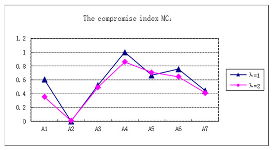
and Figure 4.

Rank the alternatives by the compromise index $M{C}_i$ of $A_i$ ($i=1,2,\dots ,7$). See

Table 19. The ranking of $A_i$.

Distance Parameter	Rank
$\lambda =1$	$A_4\succ A_6\succ A_5\succ A_1\succ A_3\succ A_7\succ A_2$
$\lambda =2$	$A_4\succ A_5\succ A_6\succ A_3\succ A_7\succ A_1\succ A_2$

.

The results of the algorithm based on Pang Qi et al.’s method [27] are as follows:

The closeness coefficient of $A_i(i=1,2,\dots ,7)$ is

$$C{I}_i=\frac{d(A_i,L^{-})}{d_{max}(A_i,L^{-})}-\frac{d(A_i,L^{+})}{d_{min}(A_i,L^{+})}$$

(23)

Calculate the closeness coefficient $C{I}_i$ by Equation (23), and obtain the results. See

Table 20. The closeness coefficient $C{I}_i$.

	Attribute	${\mathit{A}}_1$	${\mathit{A}}_2$	${\mathit{A}}_3$	${\mathit{A}}_4$	${\mathit{A}}_5$	${\mathit{A}}_6$	${\mathit{A}}_7$
Distance Parameter
$\lambda =1$		−0.2062	−0.1958	−0.1821	−0.1767	−0.1506	−0.1832	−0.1754
$\lambda =2$		−0.2585	−0.2349	−0.2251	−0.2280	−0.1903	−0.2297	−0.2103

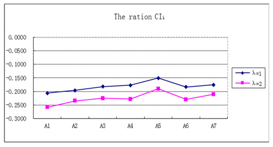
and Figure 5.

Rank the alternatives by the closeness coefficient $C{I}_i$ of $A_i$ ($i=1,2,\dots ,7$). See

Table 21. The ranking of $A_i.$

Distance Parameter	Rank
$\lambda =1$	$A_5\succ A_7\succ A_4\succ A_3\succ A_6\succ A_2\succ A_1$
$\lambda =2$	$A_5\succ A_7\succ A_3\succ A_4\succ A_6\succ A_2\succ A_1$

.

From the comparative analysis, we can find when $\lambda =1$, the ranking of $A_i$ ($i=1,2,\dots ,7$) is “$A_5\succ A_2\succ A_7\succ A_3\succ A_6\succ A_4\succ A_1$” and when $\lambda =2$, the ranking of $A_i$ ($i=1,2,\dots ,7$) is “$A_5\succ A_7\succ A_2\succ A_3\succ A_6\succ A_4\succ A_1$”, which illustrates the ranking results of the algorithm based on PT are consistent with that of the algorithm based on TOPSIS. See Table 13 and Table 17. Although the parameters $(\mathsf{\theta },\mathsf{\alpha },\mathrm{and}\mathsf{\beta })$ are changed, the ranking of $A_i$ are still “$A_5\succ A_2\succ A_7\succ A_3\succ A_6\succ A_4\succ A_1$” ($\lambda =1$) and “$A_5\succ A_7\succ A_2\succ A_3\succ A_6\succ A_4\succ A_1$” ($\lambda =2$) respectively. See Table 15 and Table 17. However, the rankings of $A_i$ are different in the other three algorithms. See Table 19 and Table 21. The comparative analysis results demonstrate the algorithm based on PT is superior to the other three traditional algorithms.

4.4. The Second Case Study

In order to illustrate the feasibility and validity of the algorithm based on PT better, a second case study is given. There are seven cars to choose on the “Auto Home” website. The seven cars are ATENZA ($A_1$), CAMRY ($A_2$), ACCORD ($A_3$), LAMANDO ($A_4$), SAGITAR ($A_5$), LAVIDA($A_6$), and BORA ($A_7$). The computational and analytical processes are the same as in Section 4.1.

Collect the users’ assessment information on the “Auto Home” website until January 5 in 2019. See

Table 22. The assessment information from scoring data by $S_5$.

Alternative	${\mathit{x}}_1$	${\mathit{x}}_2$	${\mathit{x}}_3$	${\mathit{x}}_4$	${\mathit{x}}_5$	${\mathit{x}}_6$	${\mathit{x}}_7$	${\mathit{x}}_8$
$A_1$	$S_{4.45}^5$	$S_{4.82}^5$	$S_{4.93}^5$	$S_{4.72}^5$	$S_{4.13}^5$	$S_{4.92}^5$	$S_{4.52}^5$	$S_{4.78}^5$
$A_2$	$S_{4.65}^5$	$S_{4.53}^5$	$S_{4.70}^5$	$S_{4.75}^5$	$S_{4.61}^5$	$S_{4.88}^5$	$S_{4.57}^5$	$S_{4.56}^5$
$A_3$	$S_{4.88}^5$	$S_{4.71}^5$	$S_{4.61}^5$	$S_{4.60}^5$	$S_{4.26}^5$	$S_{4.84}^5$	$S_{4.4}^5$	$S_{4.54}^5$
$A_4$	$S_{3.96}^5$	$S_{4.77}^5$	$S_{4.77}^5$	$S_{4.63}^5$	$S_{4.34}^5$	$S_5^5$	$S_{4.03}^5$	$S_{4.27}^5$
$A_5$	$S_{4.53}^5$	$S_{4.41}^5$	$S_{4.65}^5$	$S_{4.42}^5$	$S_{4.26}^5$	$S_{4.65}^5$	$S_{4.38}^5$	$S_{4.43}^5$
$A_6$	$S_{4.7}^5$	$S_{3.96}^5$	$S_{4.36}^5$	$S_{4.22}^5$	$S_{4.1}^5$	$S_{4.86}^5$	$S_{3.79}^5$	$S_{4.1}^5$
$A_7$	$S_{4.52}^5$	$S_{3.64}^5$	$S_{4.40}^5$	$S_{4.25}^5$	$S_{4.12}^5$	$S_{4.75}^5$	$S_{3.82}^5$	$S_{3.99}^5$

,

Table 23. The assessment information from word-of-mouth data by $S_7$.

Alternative	${\mathit{x}}_1$	${\mathit{x}}_2$	${\mathit{x}}_3$	${\mathit{x}}_4$	${\mathit{x}}_5$	${\mathit{x}}_6$	${\mathit{x}}_7$	${\mathit{x}}_8$
$A_1$	$S_5^7$	$-$	$S_7^7$	$S_6^7$	$S_7^7$	$S_5^7$	$S_2^7$	$S_4^7$
$A_2$	$S_7^7$	$S_2^7$	$S_3^7$	$S_6^7$	$S_6^7$	$S_6^7$	$S_7^7$	$S_5^7$
$A_3$	$S_7^7$	$S_7^7$	$S_4^7$	$S_5^7$	$S_6^7$	$S_4^7$	$S_5^7$	$S_6^7$
$A_4$	$S_3^7$	$S_7^7$	$-$	$S_6^7$	$S_4^7$	$S_7^7$	$S_5^7$	$S_6^7$
$A_5$	$S_5^7$	$S_2^7$	$S_5^7$	$S_6^7$	$S_5^7$	$S_5^7$	$S_7^7$	$S_7^7$
$A_6$	$S_4^7$	$S_1^7$	$S_7^7$	$S_6^7$	$S_6^7$	$S_7^7$	$S_1^7$	$S_5^7$
$A_7$	$S_7^7$	$S_1^7$	$-$	$-$	$S_5^7$	$S_6^7$	$-$	$S_4^7$

and

Table 24. The assessment information from forum reviews data by $S_9$.

Alternative	${\mathit{x}}_1$	${\mathit{x}}_2$	${\mathit{x}}_3$	${\mathit{x}}_4$	${\mathit{x}}_5$	${\mathit{x}}_6$	${\mathit{x}}_7$	${\mathit{x}}_8$
$A_1$	$S_7^9$	$S_7^9$	$S_8^9$	$S_4^9$	$S_4^9$	$S_9^9$	$S_3^9$	$S_4^9$
$A_2$	$S_7^9$	$S_4^9$	$S_7^9$	$S_6^9$	$S_9^9$	$S_7^9$	$S_7^9$	$S_7^9$
$A_3$	$S_8^9$	$S_7^9$	$S_6^9$	$S_3^9$	$S_7^9$	$S_8^9$	$S_6^9$	$S_7^9$
$A_4$	$S_2^9$	$S_3^9$	$S_8^9$	$S_8^9$	$S_9^9$	$S_6^9$	$S_8^9$	$S_5^9$
$A_5$	$S_8^9$	$S_4^9$	$S_8^9$	$S_3^9$	$S_2^9$	$S_9^9$	$S_9^9$	$S_5^9$
$A_6$	$S_7^9$	$S_2^9$	$S_9^9$	$S_7^9$	$S_9^9$	$S_3^9$	$S_5^9$	$S_4^9$
$A_7$	$S_1^9$	$S_5^9$	$S_8^9$	$S_7^9$	$S_7^9$	$S_7^9$	$S_7^9$	$S_7^9$

.

By the same method of Section 4.1, the weight vector $w={(w_1,w_2,w_3,w_4,w_5,w_6,w_7,w_8)}^T$ on the eight attributes $X={(x_1,x_2,x_3,x_4,x_5,x_6,x_7,x_8)}^T$ is given by Equation (12). See

Table 25. The weights of the attributes.

Attribute	$x_1$	$x_2$	$x_3$	$x_4$	$x_5$	$x_6$	$x_7$	$x_8$
Weight	0.1258	0.1774	0.1025	0.1222	0.1137	0.0953	0.1409	0.1222

.

Get the weighted DM matrix. See

Table 26. The weighted normalized DM matrix.

Alternative	${\mathit{x}}_1$	${\mathit{x}}_2$	${\mathit{x}}_3$	${\mathit{x}}_4$
$A_1$	(0.0373 0.0326 0.0300)	(0.0855,0.0690,0.0000)	(0.0342,0.0337,0.0304)	(0.0385,0.0349,0.0181)
$A_2$	(0.0419,0.0390,0.0326)	(0.0536,0.0263,0.0169)	(0.0321,0.0266,0.0146)	(0.0387,0.0349,0.0272)
$A_3$	(0.0419,0.0409,0.0373)	(0.0591,0.0591,0.0557)	(0.0315,0.0228,0.0195)	(0.0375,0.0291,0.0136)
$A_4$	(0.0332,0.0180,0.0093)	(0.0591,0.0564,0.0197)	(0.0489,0.0456,0.0000)	(0.0377,0.0362,0.0349)
$A_5$	(0.0380,0.0373,0.0300)	(0.0522,0.0263,0.0169)	(0.0318,0.0304,0.0244)	(0.0360,0.0349,0.0136)
$A_6$	(0.0394,0.0326,0.0240)	(0.0468,0.0131,0.0084)	(0.0342,0.0342,0.0298)	(0.0349,0.0344,0.0317)
$A_7$	(0.0419,0.0379,0.0047)	(0.0430,0.0329,0.0084)	(0.0456,0.0451,0.0000)	(0.0519,0.0475,0.0000)
Alternative	${\mathit{x}}_5$	${\mathit{x}}_6$	${\mathit{x}}_7$	${\mathit{x}}_8$
$A_1$	(0.0379,0.0313,0.0168)	(0.0318,0.0313,0.0227)	(0.0425,0.0157,0.0134)	(0.0389,0.0233,0.0181)
$A_2$	(0.0379,0.0349,0.0325)	(0.0310,0.0272,0.0247)	(0.0470,0.0429,0.0365)	(0.0371,0.0317,0.0291)
$A_3$	(0.0325,0.0323,0.0295)	(0.0308,0.0282,0.0182)	(0.0413,0.0335,0.0313)	(0.0370,0.0349,0.0317)
$A_4$	(0.0379,0.0329,0.0217)	(0.0318,0.0318,0.0212)	(0.0417,0.0379,0.0335)	(0.0349,0.0348,0.0226)
$A_5$	(0.0323,0.0271,0.0084)	(0.0318,0.0295,0.0227)	(0.0470,0.0470,0.0411)	(0.0407,0.0361,0.0226)
$A_6$	(0.0379,0.0325,0.0311)	(0.0318,0.0309,0.0106)	(0.0356,0.0261,0.0067)	(0.0334,0.0291,0.0181)
$A_7$	(0.0312,0.0295,0.0271)	(0.0302,0.0272,0.0247)	(0.0548,0.0538,0.0000)	(0.0475,0.0325,0.0233)

.

Since the calculation process of this example is the same as that of Section 4.1, then only the final calculation results are given as follows. See

Table 27. The relative values of $A_i$.

Alternative	Algorithm	${\mathit{A}}_1$	${\mathit{A}}_2$	${\mathit{A}}_3$	${\mathit{A}}_4$	${\mathit{A}}_5$	${\mathit{A}}_6$	${\mathit{A}}_7$
$\lambda =1$	PT ($C_i$)	0.4370	0.5545	0.6555	0.4802	0.4167	0.2644	0.3808
	TOPSIS ($C{D}_i$)	0.4966	0.5492	0.6070	0.5217	0.4790	0.3521	0.4482
	VIKOR ($M{C}_i$)	0.4458	0.9999	0.8332	0.3952	0.2124	0.1100	0.5794
	Pang Qi et al.’s method ($C{I}_i$)	−0.4627	−0.2415	−0.0000	−0.3566	−0.5358	−1.0676	−0.6659
Alternative	Algorithm	${\mathit{A}}_1$	${\mathit{A}}_2$	${\mathit{A}}_3$	${\mathit{A}}_4$	${\mathit{A}}_5$	${\mathit{A}}_6$	${\mathit{A}}_7$
$\lambda =2$	PT ($C_i$)	0.4387	0.6077	0.6942	0.4768	0.4441	0.3054	0.3709
	TOPSIS ($C{D}_i$)	0.4967	0.5755	0.6213	0.5205	0.4974	0.3916	0.4427
	VIKOR ($M{C}_i$)	0.3811	0.9999	0.9048	0.3483	0.2452	0.0824	0.3601
	Pang Qi et al.’s method ($C{I}_i$)	−0.5607	−0.1859	−0.0000	−0.4418	−0.5030	−0.9665	−0.8629

.

The ranking of $A_i$ is as follows. See

Table 28. The ranking of $A_i$.

Alternative	Algorithm	Ranking
$\lambda =1$	PT ($C_i$)	$A_3\succ A_2\succ A_4\succ A_1\succ A_5\succ A_7\succ A_6$
	TOPSIS ($C{D}_i$)	$A_3\succ A_2\succ A_4\succ A_1\succ A_5\succ A_7\succ A_6$
	VIKOR ($M{C}_i$)	$A_2\succ A_3\succ A_7\succ A_1\succ A_4\succ A_5\succ A_6$
	Pang Qi et al.’s method ($C{I}_i$)	$A_3\succ A_2\succ A_4\succ A_1\succ A_5\succ A_7\succ A_6$
Alternative	Algorithm	Ranking
$\lambda =2$	PT ($C_i$)	$A_3\succ A_2\succ A_4\succ A_5\succ A_1\succ A_7\succ A_6$
	TOPSIS ($C{D}_i$)	$A_3\succ A_2\succ A_4\succ A_5\succ A_1\succ A_7\succ A_6$
	VIKOR ($M{C}_i$)	$A_2\succ A_3\succ A_1\succ A_7\succ A_4\succ A_5\succ A_6$
	Pang Qi et al.’s method ($C{I}_i$)	$A_3\succ A_2\succ A_4\succ A_5\succ A_1\succ A_7\succ A_6$

.

This paper proposes a generalized distance measures method between two PLTs with multi-granular linguistic information, which are helpful to deal with multi-granular MAGDM problems. These distance measures improve the accuracy of multi-granular linguistic information in the MAGDM problems, even some assessment information is null. Especially, the parameter λ of the extended distance measures method is a variable, which can be used to obtain different distance measures formula according to people’s need. Under these distance measures, the extended MAGDM algorithm based on PT is proposed. From the sensitivity analyses of the parameters (θ, α, and β), we can find the ranking of the alternatives $A_i(i=1,2,\dots ,7)$ are different but only when $\alpha =0.85$, $\beta =0.85$, and $\theta =4.1$ for $\lambda =2$ and $\alpha =0.725$, $\beta =0.717$, and $\theta =2.04$ for $\lambda =2$; the results are coincident by the algorithm based on PT. The ranking results are different when the parameters ($\theta ,\alpha ,\mathrm{and}\beta )$ are changed. This result is consistent with the meaning of the parameters ($\theta ,\alpha ,\mathrm{and}\beta )$. Therefore, the algorithm based on PT proposed in Section 4.1 is illustrated to be scientific. Two case studies of purchasing a car is given to demonstrate the algorithm based on PT is valid and applied by comparing the extended TOPSIS, VIKOR, and Pang Qi et al.’s algorithms. Here, the parameters of $\delta$ and $v$ can be selected by what we need in actual problems. From the comparative analyses, we can find when $\lambda =1$, the ranking of $A_i$ ($i=1,2,\dots ,7$) is “$A_5\succ A_2\succ A_7\succ A_3\succ A_6\succ A_4\succ A_1$” and when $\lambda =2$, the ranking of $A_i$ ($i=1,2,\dots ,7$) is “$A_5\succ A_7\succ A_2\succ A_3\succ A_6\succ A_4\succ A_1$”, which illustrates the ranking results of the algorithm based on PT are consistent with that of the algorithm based on TOPSIS. See Table 13 and Table 17. Although the parameters $(\mathsf{\theta },\mathsf{\alpha },\mathrm{and}\mathsf{\beta })$ are changed, the ranking of $A_i$ are still “$A_5\succ A_2\succ A_7\succ A_3\succ A_6\succ A_4\succ A_1$” ($\lambda =1$) and “$A_5\succ A_7\succ A_2\succ A_3\succ A_6\succ A_4\succ A_1$” ($\lambda =2$) respectively. However, the rankings of $A_i$ are different in the other three algorithms. Therefore, the comparing analyses demonstrate the novelty, feasibility, and validity of the proposed MAGMD method based on PT. The novel method of MAGMD in this paper can be used to deal with some practical MAGDM problems under multi-granular probabilistic linguistic environments.

The MAGDM algorithm based on PT proposed in this paper also has some limitations: If there are too many attributes or alternatives, the size of Section 4.1 might be quite big. However, we can use some software packages to solve it, such as by crawler technology, matlab, python, and so on, so this is not a big problem in the use of this method. Whether there are more appropriate ways to measure the distances between two PLTs with multi-granular linguistic information is a valued question. There are some directions for further investigation: Firstly, how to select an appropriate parameter λ to calculate the distance between two PLTSs is a valued problem; secondly, the applications of these distance measures are interesting to research in other fields, such as cluster analysis, MCGDM problems, and so on; and finally, the linguistic information is also expressed by hesitant fuzzy numbers, interval fuzzy number, etc. to represent the fitting accuracy. These issues should be focused on further in the future.

References

- Zhou, L.G.; Chen, H.Y. Continous ordered linguistic distance measure and its application to multiple attribute group decision making. Group Decis. Negot. 2013, 22, 739–758. [Google Scholar] [CrossRef]
- Parreiras, R.O.; Ekel, P.Y.; Martni, J.S.C.; Palhares, R.M. A flexible consensus scheme for multicriteria group decision making under linguistiic assessments. Inf. Sci. 2010, 180, 1075–1089. [Google Scholar] [CrossRef]
- Grossglauser, M.; Saner, H. Data–driven healthcare: From patterns to actions. Eur. J. Prev. Cardiol. 2014, 21, 14–17. [Google Scholar] [CrossRef]
- Celotto, A.; Loia, V.; Senatore, S. Fuzzy linguistic approach to quality assessment model for electricity network infrastructure. Inf. Sci. 2015, 304, 1–15. [Google Scholar] [CrossRef]
- Tao, Z.F.; Chen, H.Y.; Zhou, L.G.; Liu, J.P. 2-Tuple linguistic soft set and its application to group decision making. Soft Comput. 2015, 19, 1201–1213. [Google Scholar] [CrossRef]
- Sengupta, A.T.; Pal, K.; Zhou, L.G.; Chen, H.Y. Fuzzy Preference Ordering of Interval Numbers in Decision Problems; Springer: Heidelberg, Germany, 2009; Volume 238, pp. 140–143. [Google Scholar]
- Zadeh, L.A. Fuzzy sets. Inf. Control 1965, 3, 338–353. [Google Scholar] [CrossRef]
- Xu, Z.S. Linguistic Decision Making: Theory and Methods; Springer: Berlin/Heidelberg, Germany, 2012. [Google Scholar]
- Herrera, F.; Verdegay, J.L. Linguistic assessments in group decision. In Proceedings of the First European Congress on Fuzzy and Intelligent Technologies, Aachen, Germany, 7–10 September 1993; pp. 941–948. [Google Scholar]
- Herrera, F.; Herrera-Viedma, E.; Verdegay, J.L. A model of consensus in group decision making under linguistic assessments. Fuzzy Sets Syst. 1996, 78, 73–87. [Google Scholar] [CrossRef]
- Herrera, F.; Herrera-Viedma, E.; Verdegay, J.L. A rational consensus model in group decision making using linguistic assessments. Fuzzy Sets Syst. 1997, 88, 31–49. [Google Scholar] [CrossRef]
- Xu, Z.S. A method for multiple attribute decision making with incomplete weight information in linguistic setting. Knowl.-Based Syst. 2007, 20, 719–725. [Google Scholar] [CrossRef]
- Arieh, D.B.; Chen, Z. Linguistic group decision-making: Opinion aggregation and measures of consensus. Fuzzy Opt. Decis. Mak. 2006, 5, 371–386. [Google Scholar] [CrossRef]
- Xu, Z.S. An approach based on the uncertain LOWG and induced uncertain LOWG operators to group decision making with uncertain multiplicative linguistic preference relations. Decis. Support Syst. 2006, 41, 488–499. [Google Scholar] [CrossRef]
- Liu, P.D.; Mahmood, T.; Khan, Q. Multi-Attribute Decision-Making Based on Prioritized Aggregation Operator under Hesitant. Symmetry 2017, 9, 11. [Google Scholar] [CrossRef]
- Liao, H.C.; Zhang, C.; Luo, L. A multiple attribute group decision making method based on two novel intuitionistic multiplicative distance measures. Inf. Sci. 2018, 467, 766–783. [Google Scholar] [CrossRef]
- Rodríguez, R.M.; Martínez, L.; Herrera, F. Hesitant fuzzy linguistic term sets for decision making. IEEE Trans. Fuzzy Syst. 2012, 20, 109–119. [Google Scholar] [CrossRef]
- Torra, V. Hesitant fuzzy sets. Int. J. Intell. Syst. 2010, 25, 529–539. [Google Scholar] [CrossRef]
- Zadeh, L.A. The concept of a linguistic variable and its application to approximate reasoning—I. Inf. Sci. 1975, 8, 199–249. [Google Scholar] [CrossRef]
- Dong, Y.C.; Wu, Y.Z.; Zhang, H.J.; Zhang, G.Q. Multi-granular unbalanced linguistic distribution assessments with interval symbolic proportions. Knowl.-Based Syst. 2015, 82, 139–151. [Google Scholar] [CrossRef]
- Wu, Z.B.; Xu, J.P. Possibility distribution-based approach for MAGDM with hesitant fuzzy linguistic information. IEEE Trans. Cybern. 2016, 46, 694–705. [Google Scholar] [CrossRef]
- Zhang, G.Q.; Dong, Y.C.; Xu, Y.F. Consistency and consensus measures for linguistic preference relations based on distribution assessments. Inf. Fusion 2014, 17, 46–55. [Google Scholar] [CrossRef]
- Liu, H.B.; Rodriguez, R.M. A fuzzy envelope for hesitant fuzzy linguistic term set and its application to multi-criteria decision making. Inf. Sci. 2014, 258, 220–238. [Google Scholar] [CrossRef]
- Yang, J.B. Rule and utility based evidential reasoning approach for multi-attribute decision analysis under uncertainties. Eur. J. Oper. Res. 2001, 131, 31–61. [Google Scholar] [CrossRef]
- Yang, J.B.; Xu, D.L. On the evidential reasoning algorithm for multiple attribute decision analysis under uncertainty. IEEE Trans. Syst. Man Cybern. Part A Syst. Hum. 2002, 32, 289–304. [Google Scholar] [CrossRef]
- Wang, J.H.; Hao, J.Y. A new version of 2-tuple fuzzy linguistic representation model for computing with words. IEEE Trans. Fuzzy Syst. 2006, 14, 435–445. [Google Scholar] [CrossRef]
- Pang, Q.; Wang, H.; Xu, Z.S. Probabilistic linguistic term sets in multi-attribute group decision making. Inf. Sci. 2016, 369, 128–143. [Google Scholar] [CrossRef]
- Lin, M.W.; Xu, Z.S.; Zhai, Y.L.; Yao, Z.Q. Multi-attribute group decision-making under probabilistic uncertain linguistic environment. J. Oper. Res. Soc. 2017, 1–15. [Google Scholar] [CrossRef]
- Xu, Z.S.; Zhou, W. Consensus building with a group of decision makers under the hesitant probabilistic fuzzy environment. Fuzzy Opt. Decis. Mak. 2017, 16, 481–503. [Google Scholar] [CrossRef]
- Lin, M.W.; Xu, Z.S. Probabilistic Linguistic Distance Measures and Their Applications in Multi-criteria Group Decision Making. In Soft Computing Applications for Group Decision-Making and Consensus Modeling; Springer: Cham, Switzerland, 2018; Volume 357, pp. 411–440. [Google Scholar]
- Kobina, A.; Liang, D.C. Probabilistic linguistic power aggregation operators for multi-criteria group decision making. Symmetry 2017, 9, 12. [Google Scholar] [CrossRef]
- Xu, Z.S.; Wang, H. Managing multi-granularity linguistic information in qualitative group decision making: An overview. Granul. Comput. 2016, 1, 21–35. [Google Scholar] [CrossRef]
- Wang, H.; Xu, Z.S.; Zeng, X.J. Hesitant fuzzy linguistic term sets for linguistic decision making: Current developments, issues and challenges. Inf. Fusion 2018, 43, 1–12. [Google Scholar] [CrossRef]
- Gorzalczany, M.B. An interval-valued fuzzy inference method-some basic properties. Fuzzy Sets Syst. 1989, 31, 243–251. [Google Scholar] [CrossRef]
- Atanassov, K.T. Intuitionistic fuzzy sets. Fuzzy Sets Syst. 1986, 20, 87–96. [Google Scholar] [CrossRef]
- Atanassov, K.T.; Gargov, G. Interval–valued intuitionistic fuzzy sets. Fuzzy Sets Syst. 1989, 31, 343–349. [Google Scholar] [CrossRef]
- Chen, N.; Xu, Z.S.; Xia, M.M. Interval-valued hesitant preference relations and their applications to group decision making. Knowl-Based Syst. 2013, 37, 528–540. [Google Scholar] [CrossRef]
- W, L.; W, Y.M.; Martinez, L. A group decision method based on prospect theory for emergency situations. Inf. Sci. 2017, 418, 119–135. [Google Scholar]
- Yao, S.; Yu, D.; Song, Y.; Yao, H.; Hu, Y.; Guo, B. Dry bulk carrier investment selection through a dual group decision fusing mechanism in the green supply chain. Sustainability 2018, 10, 4528. [Google Scholar] [CrossRef]
- Herrera, F.; Herrera-Viedma, E.; Verdegay, J.L. A sequential selection process in group decision making with a linguistic assessment approach. Inf. Sci. 1995, 85, 223–239. [Google Scholar] [CrossRef]
- Rodríguez, R.M.; Martínez, L.; Herrera, F. A group decision making model dealing with comparative linguistic expressions based on hesitant fuzzy linguistic term sets. Inf. Sci. 2013, 241, 28–42. [Google Scholar] [CrossRef]
- Yager, R.R. Generalized OWA aggregation operators. Fuzzy Opt. Decis. Mak. 2004, 3, 93–107. [Google Scholar] [CrossRef]
- Ma, J.; Fan, Z.P.; Huang, L.H. A subjective and objective integrated approach to determine attribute weights. Eur. J. Oper. Res. 1999, 112, 397–404. [Google Scholar] [CrossRef]
- Kahneman, D.; Tversky, A. Prospect theory: An analysis of decision under risk. Econometrica 1979, 47, 263–292. [Google Scholar] [CrossRef]
- Xu, Z.S.; Xia, M.M. Hesitant Fuzzy entropy and cross-entropy and their use in multi-attribute decision-making. Int. J. Intell. Syst. 2012, 27, 799–822. [Google Scholar] [CrossRef]
- Wang, L.Z.; Zhang, X.; Wang, Y.M. A prospect theory-based interval dynamic reference point method for emergency decision making. Expert Syst. Appl. 2015, 42, 9379–9388. [Google Scholar] [CrossRef]
- Zhang, X.L.; Xu, Z.S. The TODIM analysis approach based on novel measured functions under hesitant fuzzy environment. Knowl.-Based Syst. 2014, 61, 48–58. [Google Scholar] [CrossRef]
© 2019 by the author. Licensee MDPI, Basel, Switzerland. This article is an open access article distributed under the terms and conditions of the Creative Commons Attribution (CC BY) license (http://creativecommons.org/licenses/by/4.0/).