Article

Optimal Parameter Selection in Robotic Belt Polishing for Aeroengine Blade Based on GRA-RSM Method

1
School of Mechanical Engineering, Northwestern Polytechnical University, Xi’an 710072, China
2
Manufacturing Process Research Department, Xi’an Electronic Engineering Research Institute, Xi’an 710100, China
3
Robotics and Mechatronics Research Laboratory, Department of Mechanical and Aerospace Engineering, Monash University, Clayton 3800, Australia
*
Author to whom correspondence should be addressed.
Symmetry 2019, 11(12), 1526; https://doi.org/10.3390/sym11121526
Submission received: 14 November 2019 / Revised: 3 December 2019 / Accepted: 9 December 2019 / Published: 17 December 2019

Abstract

:
Due to its flexibility and versatility, robotic belt polishing is one of the most effective processing methods to improve the surface quality of aeroengine blades. Since belt polishing of blades is a material removal process aimed at reducing surface roughness, it is difficult to achieve both minimum surface roughness and maximum material removal rates. In order to solve this problem, this paper proposes an optimization method combining grey correlation analysis (GRA), the Taguchi method, and the response surface method (RSM) for the multiobjective optimization of the process parameters of Ti–6Al–4V aeroengine blade polishing. Meanwhile, the problem of the influence of asymmetry on the polishing process parameters vis-a-vis the optimization goal was solved. Experiments of robotic belt polishing for aeroengine blades were carried out. Based on the results of the principal component analysis, the grey relational grade was established to turn multiobjective optimization into single-objective optimization. A quadratic regression model of Grey correlation grade was developed, and an optimal parameter combination was obtained by the RSM. Finally, verification experiments were performed, and the combination of optimal parameters was obtained as follows: feed rate of 232.09 mm/min, compression amount of 0.08 mm, and belt line speed of 16 m/s, which reduced surface roughness by 6.29% and increased the material removal rate by 16.11%. Comparing the results of GRA-RSM and GRA, the Grey correlation grade increased by 10.96%. In other words, the goal of simultaneously reducing the surface roughness and improving the material removal rate was achieved in robotic belt polishing for aeroengine blades.

1. Introduction

Polishing techniques for workpieces with complex geometry surfaces have broad applications in fields such as aerospace, defense, electric power, and medical instruments. At present, polishing methods mainly include manual polishing, special machine polishing, and CNC machine polishing [1]. Among them, manual polishing is time-consuming and labor-intensive, and the processing yield is low. Moreover, the consistency of processing cannot be effectively guaranteed. Compared with the typical 5-axis polishing machine tool on the market, robots can be applied to large working spaces. The degree of freedom and low cost make robotic polishing more operative, as it can process workpieces with more complex surface forms [2,3]. Belt polishing is widely used in the polishing of curved parts, and is one of the most widely used finishing methods due to its properties, such as elastic polishing and strong process flexibility and adaptability [4,5,6,7]. Therefore, robotic belt polishing has become an effective method in the polishing of blades to improve the accuracy and surface quality of blade profiles.
Since the robotic belt polishing of the aeroengine blade is a material removal process for reducing surface roughness (SR), it is difficult to achieve both the minimum SR and the highest material removal rates (MRRs), which result from different polishing parameter combinations. In other words, SR and MRR may be in an asymmetric relationship to one another. Many researchers have conducted studies to improve polishing surface quality and MRR. Xiao et al. studied the surface quality of abrasive belt grinding GH4169 nickel-based superalloy material; the results indicated that the process parameter that had the greatest influence on SR was vibration frequency, followed by contact pressure and grinding speed. Meanwhile, the optimum process parameter combination was obtained [8]. Huo et al. investigated the grinding of a Ti6Al4V alloy with a superabrasive grinding wheel and analyzed the effect of the process parameters on SR. The results showed that the SR decreased with the decrease of grinding depth and increased with the decrease of the grinding wheel speed [9]. Bigerelle et al. established a wear mechanism model for abrasive belt grinding and polishing, and studied the influence of process parameters on the SR [10]. Wu et al. proposed a new MRR prediction model for robotic belt grinding, and then modeled and analyzed the two process parameters, i.e., robot movement speed and contact pressure, which affect the MRR [11]. Song et al. studied the process parameters, workpiece morphology, and mold wear that affect the removal rate of the abrasive belt in the robot polishing and proposed an offline programming method for the control of the process parameters [12]. However, the following issues remain unresolved in the robotic belt polishing of the aeroengine blade: The minimum SR and highest MRR are the result of different process parameter combinations. More importantly, the contribution rate of the process parameters to SR and MRR has not yet been studied.
The aforementioned studies only focused on single-objective optimization for SR or material removal rate, and the literature on multiobjective optimization of aeroengine blade polishing is scarce. In the field of engineering, the Grey relational analysis method is often used to establish the relationship between multi-input variables and multioutput variables to solve multiobjective optimization problems. Principal component analysis can be used to calculate the contribution rate of SR and MRR to Grey correlation, namely, influence weight. The response surface method (RSM) is used to model the relationship between the polishing process parameters and the grey correlation grade [13,14,15]. This paper adopts the comprehensive method to study the multiobjective parameter optimization problem of the aeroengine blade polishing process. The optimum process parameters obtained by the proposed method achieve an improved SR and a greater MRR in robotic belt polishing for aeroengine blades.

2. Experiment Procedure

2.1. Experimental Design

During the belt polishing process, process parameters such as feed rate, compression amount, and rotational speed affect machining efficiency and surface quality. The blade belt polishing process is shown in Figure 1. In the blade polishing process, material removal is achieved by a flexible contact between the abrasive belt and the surface of the workpiece [16]. From a macroperspective, abrasive belt polishing is a high-speed microcutting process with cumulative grinding results. The feed rate vf determines the contact time between the belt and the workpiece. The amount of compression ap causes the contact wheel to be crushed and deformed, and the belt has a change in the normal force of the workpiece. Therefore, the cutting state of the abrasive grains is greatly affected by the amount of compression, ap. The belt line speed vs determines the number of abrasive cuts involved in the polishing process. Therefore, the main influencing parameters in aeroengine blade polishing include feed rate vf, compression amount, and belt line speed vs. In order to investigate the relationship between the polishing process parameters and MRR and SR, the main influencing factors and parameter levels were selected, as shown in Table 1.
In order to reduce experimental costs and ensure sufficient data, the polishing experiment uses the Box-Benhnken design (BBD) method. The experimental results are listed in Table 2.

2.2. Experimental Materials and Experimental Preparation

The test piece of the Ti–6Al–4V material was used for the experiment. The chemical composition of Ti–6Al–4V is listed in Table 3.
Aeroengine blade polishing experiments were performed on the KR180 R2500 extra robot experimental platform. As shown in Figure 2, the robot gripped the blade and moved it closer for abrasive belt grinding. The belt drive motor had a power of 1.48 kW, and the SR of the test piece before polishing was 0.9–1.0 μm. The polishing belt was a German Hermes cloth base, with SiC abrasive and synthetic resin binder, and the belt width was 15 mm. The belt tension was controlled by a controller, the IPC-610-H-IPC, manufactured by Advantech Technology Co., Ltd, with a control cycle of 0.05 s. The collected data were displayed and processed using the LabWindows/CVI software developed by National Instruments, and the pneumatic pressure system was controlled by the command signal sent by the industrial computer to realize the real-time control of the tension of the abrasive belt. The condition was called dry polishing.

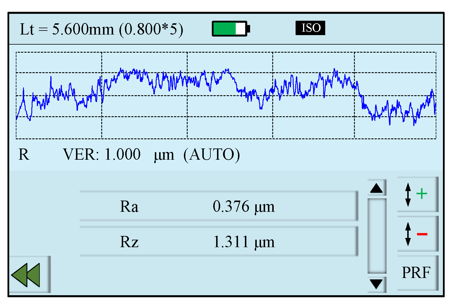
2.3. Measurement Methods

Five measurement points were selected on the machined surface before and after the polishing of each blade. The SR was measured in a direction vertical to the polishing path using a M300C surface roughness meter (sampling length of 5.6 mm), manufactured by Mahr GmbH, as shown in Figure 3. The average measured value of the SR, Ra, was selected as the final result of the SR.
In this paper, the MRR was indirectly determined by measuring the change in blade thickness. The thickness of the blade was measured using a 395–271 electronic digital micrometer (resolution 1 μm, measuring range 0–25 mm), manufactured by Mitutoyo Corporation. The MRR was computed as follows [17]:
Zw = v f Δ h   P n B ,
where Zw is the MRR (mm2/min), vf is the feed rate, ∆h is the blade thickness variation (mm), P is the programmed track pitch (mm), n is the number of polishing times, and B is the belt width (mm).

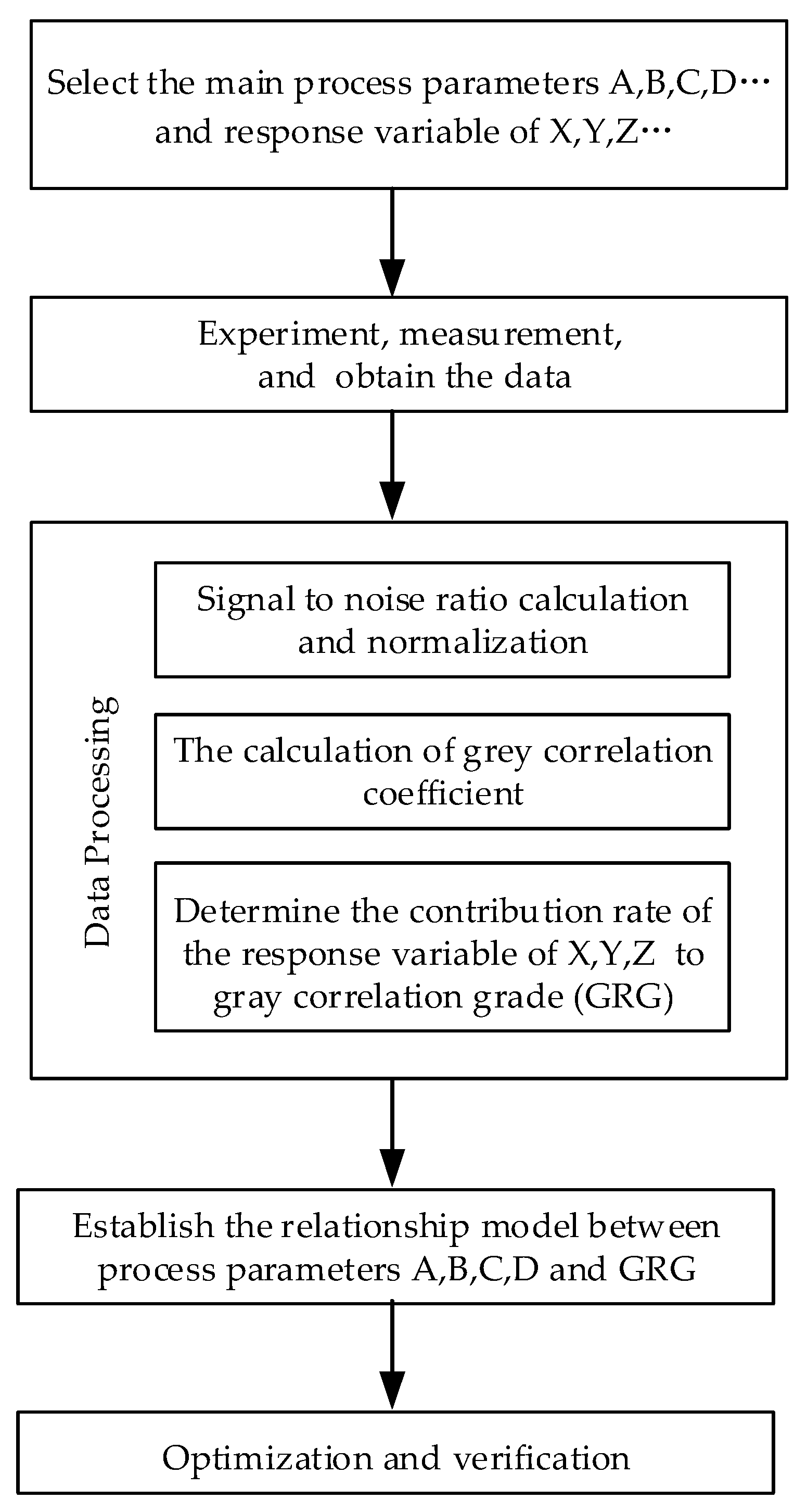
3. Multiobjective Optimization Method

The optimization method of this paper was a multiobjective optimization method integrating gray relational analysis, the Taguchi method, and RSM. In the gray correlation analysis, the signal-to-noise (S/N) ratio of SR and MRR was used as a performance indicator. Therefore, based on the gray relational grade (GRG), the multiobjective optimization problem of robotic belt polishing for aeroengine blades was simplified to a single-objective optimization problem [15]. Furthermore, an RSM model was used to establish a mapping relationship between the polishing process parameters and GRG. The detailed optimization process is as follows.
Step 1: S/N ratio calculation
The S/N ratio was used to quantify the effect of noise on the quality characteristics. For the target value of the SR, the smaller the roughness value, the better quality the characteristics; and for the processing efficiency of the quality characteristics, the larger the MRR, the better the productivity. Therefore, the S/N ratio of SR can be described as [18]
η = 10   log 10 ( 1 N i = 1 N R a i 2 ) ,
The S/N ratio of MRR can be described as [18]
η = 10 log 10 ( 1 N i = 1 N 1 Z w i 2 ) i = 1 ,   2 ,   , N ,
where Rai and Zwi are the values of SR and MRR for the i-th test, respectively.
Step 2: Normalization
Data preprocessing was performed for the S/N ratio of SR and MRR, as shown in Table 2. A larger S/N ratio corresponds to a greater quality characteristic, despite the type of quality characteristics. Therefore, two quality characteristics of SR and MRR can be converted into a “larger-the-better characteristic” standard based on the S/N ratio. The original sequence of the S/N value was normalized as follows [18]:
x i * ( k ) = x i o ( k ) min x i o ( k ) max x i o ( k ) min x i o ( k ) ,
where x i o (k) is the initial sequence of S/N ratio values, and x i * (k) is the compared sequence, where k = 1, 2, …, q; i = 1, 2, …, p; here, p and q are, respectively, the number of experiments and the corresponding number of goals.
Step 3: Calculation of the gray correlation coefficient
Assuming that x 0 * (k) is the reference sequence, the gray relation coefficient can be defined as follows [18]:
γ ( x 0 * ( k ) ,   x i * ( k ) ) = Δ min + λ Δ max Δ 0 i ( k ) + λ Δ max ,   0 < γ ( x 0 * ( k ) ,   x i * ( k ) ) 1 ,
where △0i(k) is the corresponding deviation sequence for the reference sequence x 0 * (k) and the compared sequence x i * (k), namely Δ0i(k) =| x 0 * (k) − x i * (k)|, Δmax = i m a x j m a x Δ0i(k), Δmin = i m i n j m i n Δ0i(k), and λ is the resolution coefficient, λ ∈ [0,1].
Step 4: Determination of the weight of the response variable
Principal component analysis was used to assess the contribution rate of SR and MRR to the gray correlation in this paper [19].
Step 5: Gray correlation calculation
The weighted sum of all gray correlation coefficients is the gray correlation degree. Its calculation formula is as follows [18]:
γ ( x 0 * , x i * ) = k = 1 n β k γ ( x 0 * ( k ) ,   x i * ( k ) ) ,
where γ( x 0 * , x i * ) represents the degree of association of the reference sequence x 0 * (k) and the comparison sequence x i * (k). Therefore, the greater the degree of gray correlation, the closer the matching parametric combination to the optimal value of the response variable. In addition, the gray correlation degree also indicates the influence level of the parameter level on the quality characteristics. βk is the weight factor of the k-th response variable, and is derived from the results of the principal component analysis in Step 4.
Step 6: Model building and verification
A multivariate quadratic model of GRG was constructed to characterize the relationship between GRG and process parameters. The control parameters were selected in the random range for verification experiments in order to prove the prediction accuracy of the model.
Step 7: Parametric optimization
The best combination of process parameters was determined from the demand analyses.
Step 8: Performance of a verification test
In order to express the optimization method more clearly and to make more readers understand and use this method, a flowchart is shown in Figure 4.

4. Results and Discussion

4.1. Effect of Polishing Parameters on a Single Response Variable

The raw data were preprocessed after the blade polishing experiment. First, the Taguchi method was used to convert the experimental data of two responses into an S/N ratio. The advantage of this data transformation is that multiobjective optimization of SR and MRR can be translated to maximize the S/N ratio. The processing results listed in Table 2 were obtained by Equations (2) and (3).
Table 4 shows the average S/N ratio for a single response variable. The belt line speed vs was the main process parameter affecting SR, followed by the amount of compression ap; the feed rate vf had little effect on SR. The amount of compression ap was the main process parameter affecting the MRR, followed by the belt line speed vs. The feed rate vf had the same effect on the MRR. The main reason for the small influence of the feed rate vf on SR and MRR was that the feed rate vf was sufficiently small relative to the belt line speed vs, so the change in feed rate vf had little effect on the speed of the synthesis of the abrasive particles involved in polishing.

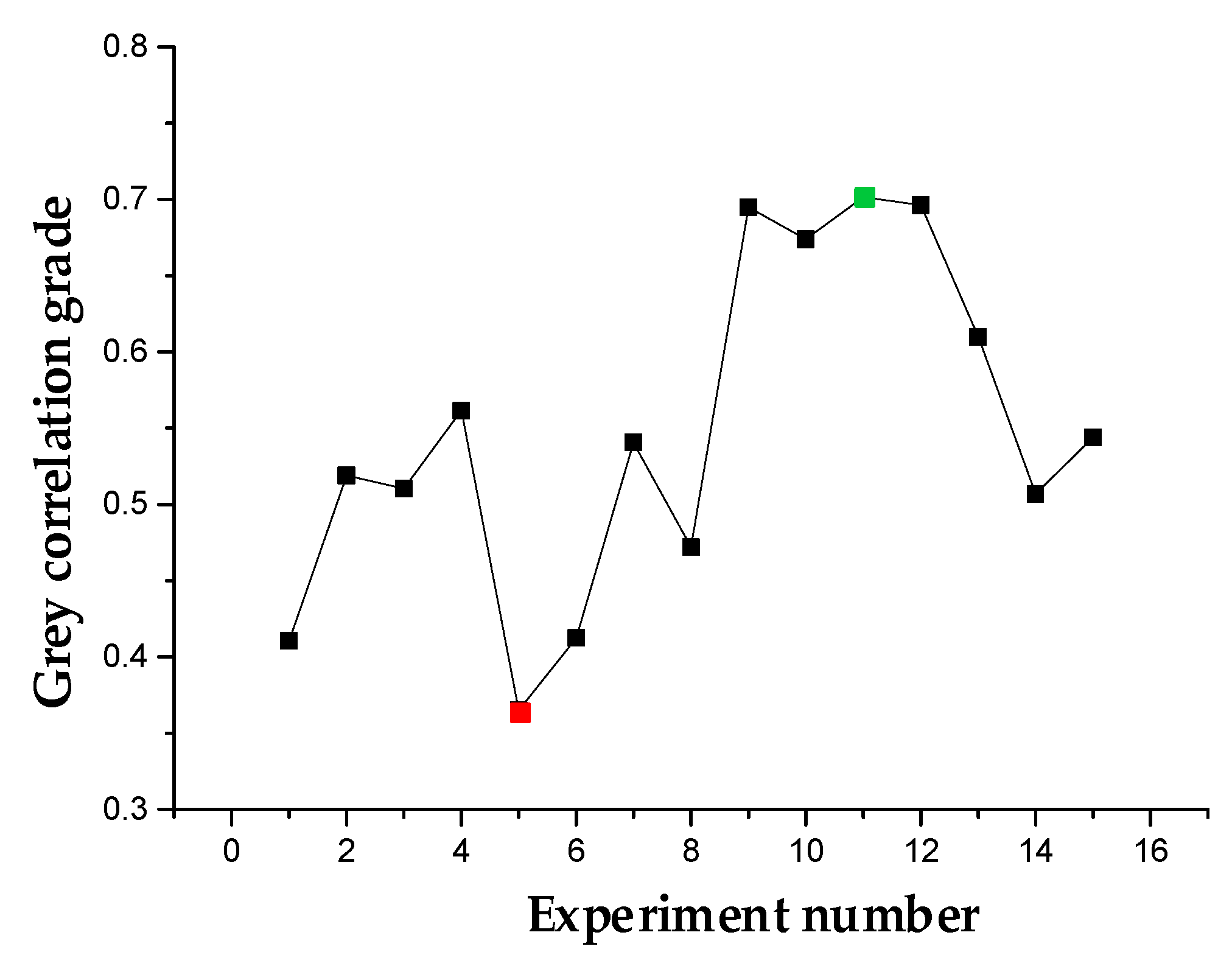
4.2. Gray Correlation Analysis

According to the standard of the larger-the-better characteristic, the S/N ratio was normalized in the interval [0,1] by Equation (4). Next, △0i(k), the deviation sequence, was calculated according to Step 3. Then the gray relation coefficient was determined by Equation (5), wherein the resolution coefficient λ was set to 0.5. The results are presented in Table 5.
Before calculating the GRG, it is necessary to confirm the weight value βk of each response variable. Principal component analysis was used in this study to determine the weight of SR and MRR [16]. As listed in Table 6, SR is the priority principal component, followed by MRR. The corresponding contribution rates were 54.6% and 45.4%, respectively. Therefore, the weight values β1 and β2 were 0.546 and 0.454. The gray correlation degree was calculated by Equation (6). Table 5 converts multiple responses to a single goal. The larger the GRG, the closer the value to the desired quality characteristic value. Figure 5 shows the value of GRG, and the maximum value (0.7014) was found in the 11th experiment. The results show that in 15 tests, the combination of a feed rate of 200 mm/min, a compression of 0.08 mm, and a belt line speed of 16 m/s achieved the best multiresponse characteristics. A minimum was found in the fifth experiment. This indicates that the worst parametric combination condition was a feed rate of 100 mm/min, a compression of 0.05 mm, and a spindle speed of 8 m/s.

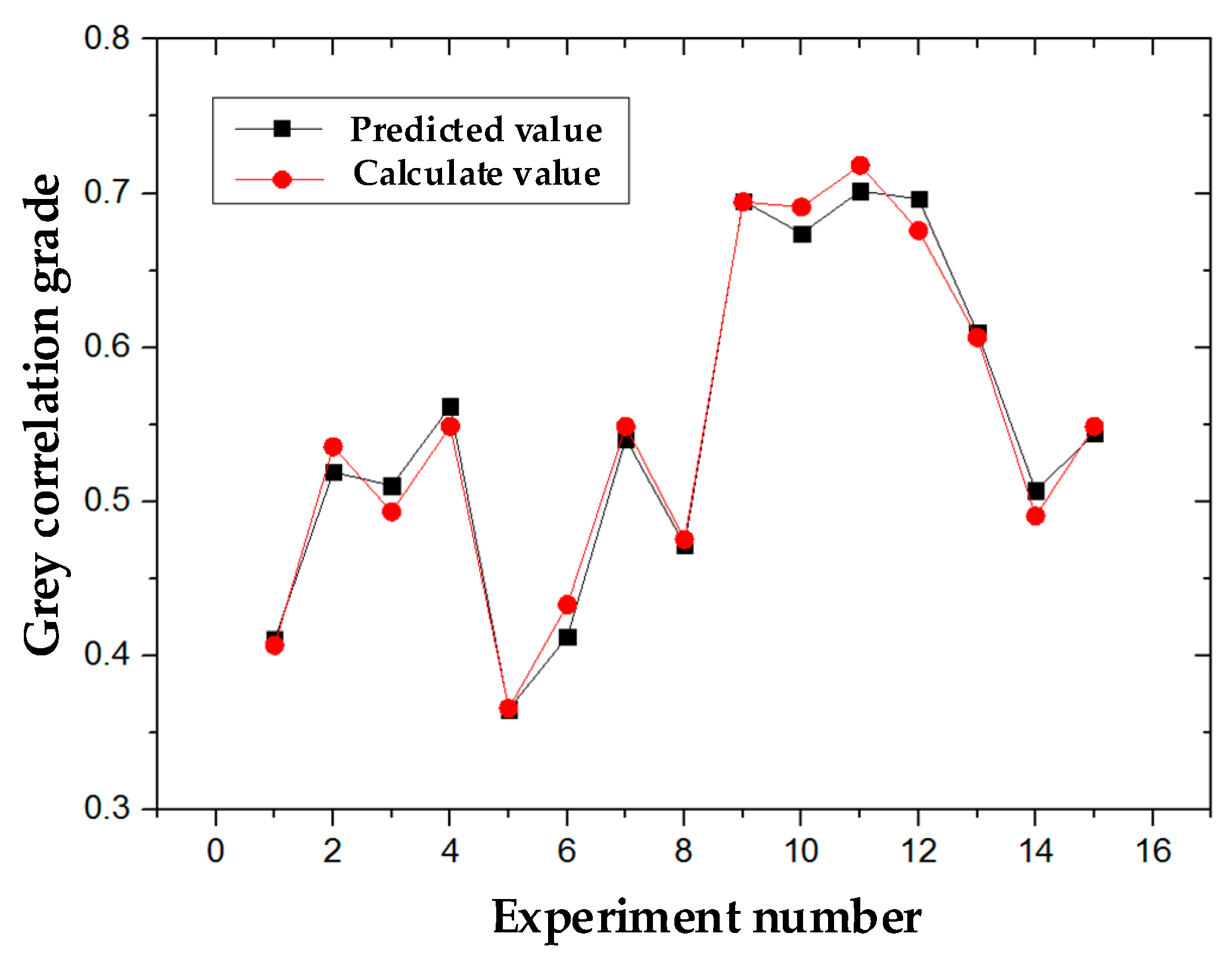
4.3. Model Establishment

After obtaining GRG, we established a mapping relationship between GRG and the process parameters. In this paper, the RSM method was used to build and optimize the GRG model. According to the BBD design experiment, the secondary model of the response surface was used to reflect the degree of influence of the process parameters. The RSM model was obtained as follows:
GRG = 0.14205 + 1.79891 × 10⁻³ vf − 1.12643 ap − 2.93385 × 10⁻³ vs + 4.6518 × 10⁻³ vf × ap
    − 3.05046 × 10⁻⁵ vf × vs + 5.42413 × 10⁻⁵ ap × vs − 3.62566×10⁻⁶ vf2 + 15.99582 ap2
+ 1.85397 × 10⁻³ vs2                       
Figure 6 shows a comparison of the calculation results and the prediction results of GRG, which indicates that the predictive model is feasible. Hence, the modified second-order model can be considered to navigate the design space.

4.4. Optimal Gray Correlation Prediction

In order to illustrate the influence of polishing process parameters on gray relational grade more visually, the response profile of the GRG related to the design variables is plotted in Figure 7 based on the quadratic regression model. The expected function was used for the GRG value in this study. The goal was to search for the maximum value between 0.3649 and 1. Using the Design-Expert statistical software developed by Stat-Ease Inc., a combination of process conditions was selected with the highest satisfaction values as the best condition for the goal. Figure 8 shows the desirable values for the goal. The points on each slope reflect the level of process parameter settings, and the height of the points describes the desirability degree. As shown in Figure 8, the optimum conditions were selected as follows: the feed rate vf was 232.09 mm/min, the compression amount ap was 0.08 mm, and the belt line speed vs was 16 m/s. Meanwhile, the corresponding optimal solution of the gray correlation degree was GRG = 0.784105.

4.5. Verification

Once the optimal process parameter level was determined, the validation experiment was performed to verify the best solution. In order to compare with the largest GRG in the designed experimental process, the highest value of GRG in the fifth experiment was selected as the original process condition setting. The results of the comparison between the optimal settings and the original settings are listed in Table 7. The results show that this method could be used to simultaneously reduce the SR of the polished blade and increase the material removal rate.

5. Conclusions

Aeroengine blade polishing is a multi-input, multiresponse process. In this paper, a multiobjective optimization algorithm integrating the Taguchi method, the gray correlation analysis, and the RSM was applied to solve the optimization problem of the processing parameters in the robotic belt polishing for aeroengine blades. The following conclusions can be drawn:
  • In the robotic belt polishing for aeroengine blades, the main parameters influencing the aeroengine blade polishing include feed rate vf, compression amount ap, and belt line speed vs. The belt line speed vs is the main process parameter affecting material removal rates and surface roughness.
  • The results of principal component analysis show that surface roughness is the priority principal component, then followed by material removal rate. The corresponding contribution rates were 54.6% and 45.4%, respectively. The proposed GRA-RSM method can effectively predict the optimal setting of process parameters in the robotic belt polishing for aeroengine blades, then achieving the important aim of reducing the surface roughness, and improving the material removal rate simultaneously.
  • For the maximum grey correlation grade, which increased by 10.96%, the optimum polishing parameter combination was selected as follows: the feed rate vf is 232.09 mm/min, the compression amount ap is 0.08 mm, and the belt line speed vs is 16m/s. Finally, the surface roughness was reduced by 6.29%, and the material removal rate was increased by 16.11%.

Author Contributions

J.G. introduced the concepts of this paper and collected corresponding references. P.Z. and J.G. conducted the experimental work, took part in data acquisition. T.Y., Z.C. and Y.S. participated in research design, data acquisition, data analysis and manuscript preparation. Finally, J.G. analyzed and interpreted the data, B.S. and P.Z. reviewed this paper and made constructive comments. All the authors approved and read the final manuscript.

Funding

This paper was supported by the Major Projects of Aero Engines and Gas Turbines (grant No. 2017-VII-0002-0095) and Innovation Foundation for Doctor Dissertation of Northwestern Polytechnical University (CX201946).

Conflicts of Interest

The authors declare no conflict of interest.

References

  1. Moumen, M.; Chaves-Jacob, J.; Bouaziz, M.; Linares, J.M. Optimization of pre-polishing parameters on a 5-axis milling machine. Int. J. Adv. Manuf. Technol. 2016, 85, 443–454. [Google Scholar] [CrossRef] [Green Version]
  2. Huang, H.; Gong, Z.M.; Chen, X.Q.; Zhou, L. Robotic grinding and polishing for turbine-vane overhaul. J. Mater. Process. Technol. 2002, 127, 140–145. [Google Scholar] [CrossRef]
  3. Márquez, J.J.; Pérez, J.M.; Rıos, J.; Vizán, A. Process modeling for robotic polishing. J. Mater. Process. Technol. 2005, 159, 69–82. [Google Scholar] [CrossRef]
  4. Xiao, G.; Huang, Y. Equivalent self-adaptive belt grinding for the real-R edge of an aero-engine precision-forged blade. Int. J. Adv. Manuf. Technol. 2016, 83, 1697–1706. [Google Scholar] [CrossRef]
  5. Xiao, G.; Huang, Y. Micro-stiffener surface characteristics with belt polishing processing for titanium alloys. Int. J. Adv. Manuf. Technol. 2019, 100, 349–359. [Google Scholar] [CrossRef]
  6. Xiao, G.; Huang, Y.; Wang, J. Path planning method for longitudinal micromarks on blisk root-fillet with belt grinding. Int. J. Adv. Manuf. Technol. 2018, 95, 797–810. [Google Scholar] [CrossRef]
  7. Xiao, G.; Huang, Y.; Fei, Y. On-machine contact measurement for the main-push propeller blade with belt grinding. Int. J. Adv. Manuf. Technol. 2016, 87, 1713–1723. [Google Scholar] [CrossRef]
  8. Xiao, G.; Huang, Y.; Yang, Y.H.; Yi, H. Workpiece surface integrity of GH4169 Nickel-based Superalloy when employing abrasive belt grinding method. Adv. Mater. Res. 2014, 936, 1252–1257. [Google Scholar] [CrossRef]
  9. Huo, W.G.; Xu, J.H.; Fu, Y.C.; Qi, H.J.; Shao, J. Investigation of surface integrity on dry grinding Ti6Al4V alloy with super-abrasive wheels. J. Shan. Univ. 2012, 42, 100–104. [Google Scholar]
  10. Bigerelle, M.; Gautier, A.; Hagege, B.; Favergeon, J.; Bounichane, B. Roughness characteristic length scales of belt finished surface. J. Mater. Process. Technol. 2009, 209, 6103–6116. [Google Scholar] [CrossRef]
  11. Wu, S.; Kazerounian, K.; Gan, Z.; Sun, Y. A material removal model for robotic belt grinding process. Mach. Sci. Technol. 2014, 18, 15–30. [Google Scholar] [CrossRef]
  12. Song, Y.; Liang, W.; Yang, Y. A method for grinding removal control of a robot belt grinding system. J. Intell. Manuf. 2012, 23, 1903–1913. [Google Scholar] [CrossRef]
  13. Wang, P.; Zhu, Z.; Wang, Y. A novel hybrid MCDM model combining the SAW, TOPSIS and GRA methods based on experimental design. Inform. Sci. 2016, 345, 27–45. [Google Scholar] [CrossRef]
  14. Verma, R.; Singh, N.P. GRA based network selection in heterogeneous wireless networks Wireless. Pers. Commun. 2013, 72, 1437–1452. [Google Scholar] [CrossRef]
  15. Du, S.; Chen, M.; Xie, L.; Wang, X. Optimization of process parameters in the high-speed milling of titanium alloy TB17 for surface integrity by the Taguchi-Grey relational analysis method. Adv. Mech. Eng. 2016, 8, 1–12. [Google Scholar] [CrossRef] [Green Version]
  16. Xiao, G.; Huang, Y. Two-Level Static Floatation Tool Used in Belt Grinding for Root Fillet of Titanium Alloy Blade. IEEE Access 2019, 7, 28663–28671. [Google Scholar] [CrossRef]
  17. Chen, Z.; Shi, Y.; Lin, X. Evaluation and improvement of material removal rate with good surface quality in TC4 blisk blade polishing process. J. Adv. Mech. Des. Syst. Manuf. 2018, 12, 1–12. [Google Scholar] [CrossRef]
  18. Kang, C.; Shi, Y.; He, X.; Yu, T.; Deng, B.; Zhang, H.; Sun, P. Multi-response optimization of T300/epoxy prepreg tape-wound cylinder by grey relational analysis coupled with the response surface method. Mater. Res. Exp. 2017, 4, 1–13. [Google Scholar] [CrossRef]
  19. Ray, A. Optimization of process parameters of green electrical discharge machining using principal component analysis (PCA). Int. J. Adv. Manuf. Technol. 2016, 87, 1299–1311. [Google Scholar]
Figure 1. Schematic diagram of the blade belt polishing process.
Symmetry 11 01526 g001
Figure 2. Robotic belt polishing experiment.
Symmetry 11 01526 g002
Figure 3. Surface roughness measurement result.
Symmetry 11 01526 g003
Figure 4. Flowchart of the optimization method.
Symmetry 11 01526 g004
Figure 5. Plot of GRG values.
Symmetry 11 01526 g005
Figure 6. Comparison of experimental and predicted GRG.
Symmetry 11 01526 g006
Figure 7. Parametric influence on GRA.
Symmetry 11 01526 g007
Figure 8. Ramp function graph of desirability.
Symmetry 11 01526 g008
Table 1. The level of polishing process parameters.
Experimental ParametersSymbolUnitsLevels of Experimental Parameters
Level 1Level 2Level 3
Feed ratevfmm/min100200300
Compressionapmm0.020.050.08
Belt line speedvsm/s81216
Table 2. Experimental design and measurement results.
NumberExperiment ParametersSRMRR
vfapvsRa (μm)S/NZw (mm²/min)S/N
12000.0280.4157.63900.0123−38.2019
21000.08120.4486.97440.0374−28.5426
32000.0880.5275.56380.0428−27.3711
42000.05120.3838.33600.0337−29.4474
51000.0580.5585.06730.0181−34.8464
63000.0580.5435.30400.0262−31.6340
72000.05120.4077.80810.0351−29.0939
81000.02120.4137.68100.0234−32.6157
93000.05160.3948.09010.0574−24.8218
102000.02160.31110.14480.0193−34.2889
112000.08160.4137.68100.0701−23.0856
121000.05160.3479.19340.0457−26.8017
133000.08120.4766.44790.0547−25.2403
143000.02120.4037.89390.0281−31.0259
152000.05120.4217.51440.0381−28.3815
Table 3. Chemical composition of Ti-6Al-4V.
Chemical CompositionAlVFeSiCNHOOther
%5.5–6.83.5–4.5≤0.30≤0.15≤0.10≤0.05≤0.01≤0.200.11
Table 4. The average S/N ratio for the levels of individual response.
SourceProcess Parameters
vfapvs
SR
Level 17.22908.33975.8935
Level 27.81247.33057.5222
Level 36.93406.66688.7773
Max-min0.87851.67292.8838
Rank321
Optimal levelA2B1C3
MRR
Level 1−30.7016−34.0331−33.0134
Level 2−29.9815−29.2895−29.1924
Level 3−28.1805−26.0599−27.2495
Max-min2.52117.97325.7639
Rank312
Optimal levelA3B3C3
Table 5. Results for gray relational analysis.
NumberDeviation Sequence Δ0iGray Relational CoefficientsGray Relational Grades
SRMRRSRMRR
10.49351.00000.50330.33330.4105
20.62440.36100.44470.58070.5190
30.90220.28350.35660.63820.5103
40.35620.42090.58400.54300.5616
51.00000.77800.33330.39120.3649
60.95340.56550.34400.46930.4124
70.46020.39750.52070.55710.5406
80.48520.63040.50750.44230.4719
90.40470.11490.55270.81320.6949
100.00000.74111.00000.40290.6740
110.48520.00000.50751.00000.7014
120.18740.24580.72740.67040.6963
130.72810.14250.40710.77820.6097
140.44330.52530.53000.48770.5069
150.51810.35030.49110.58800.5440
Table 6. The results of the principal component analysis.
Principal ComponentEigenvalueContribution
SR1.092454.6%
MRR0.9047645.4%
Total 100%
Table 7. Comparison of the original and optimal setting.
Initial Factor SettingOptimal Process ConditionImprovement
PredictionValidation
vf200 mm/min232.09 mm/min232.09 mm/min
ap0.08 mm0.08 mm0.08 mm
vs16 m/s16 m/s16 m/s
SR0.413 μm 0.387 μm6.29%
MRR0.0701 mm²/min 0.0814 mm²/min16.11%
GRG0.70140.78410.778310.96%

