1. Introduction
The human ear provides a robust source of biometric information with several desirable characteristic features that could be exploited in personal identification, overcoming the drawbacks of other biometric modalities and enriching the biometric technology. These characteristic features are categorized into three levels based on the type of features recognized by either human experts or machines [
2]. The first level of features is concerned with the general description of the ear appearance such as ear shape and skin color. These features could be extracted from ear images at low resolution. Even though these features are useful for classification or in the early process of subject elimination due to a totally different appearance, they are not adequate to recognize a person over a large number of candidates with similar looking ear images. The second level of features, which is essential for recognition, describes the geometric ear structure with localized ear characteristics such as ear curvature, edges, folds, ridges, and the relative distance between specific ear parts. In fact, these features are spatially distinct among individuals and give the ear its uniqueness to distinguish even identical twins [
3]. These types of features are extracted locally by applying a feature extraction method over sub-regions of the ear image and then concatenating them to obtain a global ear image description. The third level of ear features represents the unstructured micro features such as moles, piercings, and birthmarks, which provide supplementary information that could improve the matching accuracy in ear based recognition systems. The personal identification is performed based on such distinguishing ear characteristic features that are unique with respect to location, size, direction, and angles for each individual. This is also consolidated given the stability of the anatomical features of the ear, which do not change dramatically during human life.
In its beginnings, identity recognition with ear images was dominated by the combination of pre-defined features and the subsequent use of traditional machine learning classifiers. The feature extraction process is arguably the most important phase in the recognition process where the main task is to describe the ear characteristics in a more distinctive way. The output of the feature extraction process is a feature vector that encodes a particular image aspect such as texture, shape, color, etc., where the image pixels are only used as input to the feature extraction method. The feature vectors are then used to train a classifier to learn the underlying patterns of the extracted feature vectors and obtain a suitable model. The most successful and widely used hand designed features in the literature are those that extract local patterns and count their distribution across the entire image. These methods encode textural and gradient based information as discriminative features. In this work, we consider the top performing representatives from both texture based and gradient based descriptors and explore their discriminative power and robustness.
Currently, deep learning methods [
4] have been developing at a fast pace and have become a popular data driven learning strategy for various computer vision tasks. They combine both traditional steps: feature extraction and classification are learned together in an end-to-end model. A typical deep learning model for feature learning is Convolutional Neural Networks (CNNs), which are composed of stacking multiple layers on top of each other and, when applied to images, automatically learn a set of filters that provide discriminative features. The filters in the lower layers of the CNN learn more generic features such as edges and corners, whereas the filters at higher layers utilize the low level features to learn more complex and abstract features capable of differentiating between individuals or different image classes. The CNNs have direct access to the raw image pixels and learn the features automatically during the network training process. In this scenario, the CNN is free to use all levels of features and learn more semantic information from the given ear images. Moreover, training a deep CNN comes with the additional advantage of tuning the representation of the input data to suit the particular problem. Furthermore, the benefits of training and learning the features lead to the high adaptiveness of deep learning strategies.
In order to learn better visual representations and subsequently improve the recognition performance, deep CNNs require large labeled datasets [
5]. However, there are certain situations when solving real-world problems where the available training data are limited and large datasets do not exist. In these cases, applying deep learning methods is not a feasible option, and conventional feature extraction and classification techniques could be a proper solution. One feasible solution for recognition problems when the amount of data are insufficient is pretraining on a similar recognition task using large scale datasets such as ImageNet [
6], as conducted in [
7,
8,
9,
10,
11]. This technique is referred to as transfer learning and has proven to be effective in plenty of application domains including ear recognition [
12,
13,
14]. In the context of deep CNNs, two types of transfer learning are applicable. First, the CNN is trained for a specific recognition task where the network learns a set of discriminating filters. Then, the learned filters can be reused to extract discriminative features for a new recognition task by treating the pretrained CNN as an arbitrary feature extractor. The extracted features can then be used to train conventional classifiers such as support vector machines as explored in [
15] or a set of fully connected layers as conducted in [
14]. Second, instead of using the pretrained CNN as a feature extractor, fine tuning replaces the top layer(s) with new one(s) and allows the weights of the pretrained network to be adapted using domain specific data. Another effective approach to improve the recognition performance is to combine multiple types of features or classifiers. The authors in [
16] employed a score based fusion of multiple CNNs and handcrafted features to improve the classification accuracy. Similarly, in [
17], handcrafted features were first extracted by representative descriptors, and an SVM was trained individually for each descriptor. The different SVMs were then combined with an ensemble of fine tuned CNNs. The obtained classification system indicated discriminative power and generalization ability across various datasets. With respect to ear recognition, Hansley et al. [
18] achieved outstanding performance in unconstrained ear recognition by fusing handcrafted and CNN learned features. The handcrafted and CNN descriptors appeared to learn different, but complementary features when combined to improve the recognition performance. For a summary of the different fusion techniques explored in ear recognition, the reader is referred to the extensive review in [
19].
In this paper, we study and compare the recognition performance of seven conventional and four deep learning based ear recognition models on three ear datasets having a limited amount of ear images acquired under controlled and uncontrolled settings. For the conventional approaches, we explore the characteristics of seven top performing handcrafted descriptors to represent the ear image in the form of a feature vector quantifying the image contents. Then, we train linear SVMs on the extracted feature vectors to obtain a suitable model to recognize the identity of unseen ear images (i.e., the test set). On the other hand, we introduce four ear recognition models based on a variant of AlexNet [
20] after specific hyperparameter optimization to suit the variable image sizes in the considered ear datasets. We experiment with different feature learning strategies including: (1) training the network from scratch to learn the most discriminative ear features, (2) using a pretrained network as a feature extractor by freezing the weights for the feature extraction part (i.e., the convolutional layers) while adjusting the classification part of the network (i.e., the fully connected layers), (3) adding a specific batch normalization layer to normalize the input to the convolutional and fully connected layers, and (4) performing domain adaptation or fine tuning of the pretrained network weights along with the inserted batch normalization layers using the training data from each dataset to learn more ear specific features. The experimental results indicate the supremacy of the CNN based models compared to the traditional techniques on the three datasets. To better interpret the obtained results, we employ the t-distributed Stochastic Neighboring Embedding (t-SNE) [
21] dimensionality reduction and visualization technique to visualize the features by mapping them onto a 2D space. The visualization provides insights on the invariance property of the CNN features with respect to some image transformations such as horizontal flipping.
The remainder of the paper is organized as follows.
Section 2 discusses the related work from the literature. In
Section 3, we explain the best performing handcrafted descriptors to describe ear images.
Section 4 presents the AlexNet architecture along with the custom changes made to suit ear recognition. In
Section 5, we describe in detail the experimental setup, benchmark datasets, evaluation protocols, and the obtained results. Finally,
Section 6 derives our main conclusions and the future research directions.
2. Related Work
For the ear recognition problem, several approaches have been proposed in the literature. These techniques are classified into four main categories based on the employed feature extraction method [
22]. The first category includes geometric techniques that consider the geometrical parts of the ear as discriminating features [
23,
24,
25]. A common approach is to apply an edge detector to describe edges from the ear image. The edges can be subsequently used to derive geometric descriptors for recognition. Although geometric features could provide robustness against rotation, scaling, and viewpoint changes, texture information is barely considered and potentially discriminative information is ignored. The second category includes holistic approaches, which encode the global appearance of the ear and compute representations that describe the entire ear image. However, these techniques are very sensitive to changes in the image appearance such as head poses or illumination; thus, some normalization techniques should be applied before computing the features. Examples for holistic approaches are given in [
26,
27,
28,
29]. The third category includes techniques that describe local image regions as discriminative features for recognition. The description can be computed for some salient points in the image or computed densely for every pixel in the entire image (as described in
Section 3). The local techniques that compute dense description of the input images are favored due to their computational simplicity and superior recognition performance as reported in several studies [
18,
30,
31,
32,
33]. The last category includes hybrid methods, which combine geometric, holistic, local, or various features in order to obtain even more discriminative descriptors. However, the increased discriminative power comes at additional computational cost.
Pattern recognition is now shifting from conventional handcrafted features to learned or CNN based image features [
34,
35,
36]. Moreover, recent advancement has pushed the research area to study the recognition performance under more challenging conditions commonly referred to as unconstrained or in the wild. However, moving from controlled to unconstrained image conditions represents the limitations for the existing ear recognition systems as reported by different evaluation groups [
37,
38]. Under the uncontrolled conditions, the recognition systems are confronted with real-world challenges such as variations in viewing angles, low resolution images, illumination variations, and occlusions caused by hair, earrings, and other objects. In order to tackle these challenges, a robust and more discriminative description of ear image features is crucial. In this study, we explore and compare the discriminative power of handcrafted and CNN descriptors to describe ear images.
Similar to our work, the authors in [
39] compared the recognition performance of three local texture descriptors. The conducted study considered only three handcrafted features, and no CNN features were used. Furthermore, the experiments were conducted on ear images from three datasets acquired under controlled conditions with slight variations in lighting.
Another comparative study was introduced in [
30]. The authors evaluated and compared the recognition performance of texture and surface descriptors. They tried different combinations of textural features with subspace projection methods and using different distance measures. The Mathematical Analysis of Images (AMI) ear dataset was used, but only 500 images out of the 700 ear images were selected. Thus, the reported results were based on a subset of the AMI dataset. Further, neither CNN features nor images acquired under uncontrolled image conditions were used.
A similar study was conducted using eight handcrafted features in [
31] and extended in [
32] to include three deep learning models based on pretrained networks. The authors re-trained the networks using separate training images to fine tune their weights. Then, the fine tuned networks were used as black-box feature extractors to obtain a feature vector for each ear image. The Annotated Web Ear (AWE) dataset was used for evaluation and the cosine distance to match the extracted feature vectors. The focus of the conducted study was to evaluate the impact of several ear image covariates such as gender, ethnicity, accessories, and different head poses on the identification performance. The reported analysis showed a significant drop in the recognition performance in the presence of accessories and a high degree of pose variations, while the impact was less for other covariates such as gender and ethnicity. On the contrary, our focus here is the exploration of handcrafted features against different types of CNN features extracted from a variant of AlexNet for different ear datasets. Furthermore, instead of relying on a distance metric for matching the extracted feature vectors, the features are classified by training SVMs on the training set and the results are reported on the test set.
Almisreb et al. [
40] introduced an ear recognition approach by fine tuning a pretrained AlexNet model. The ear images were acquired with a smart phone for 10 subjects where each subject had 30 images. The images were for the left and right ear and exhibited easy degrees of rotation and scaling effects. They used 25 images from each individual to fine tune their model and five images for testing and reporting the recognition performance. In contrast, our study is more comprehensive and includes various learning strategies. Furthermore, three datasets are used with more data, subjects, and more challenging ear images. Moreover, seven top performing handcrafted features are included along with visualization for the extracted features to substantiate the comparison.
Recently, the authors in [
41] conducted a comparative experimental study to evaluate the recognition performance of several variants of the Local Binary Pattern (LBP) texture descriptor [
42]. The authors used four ear datasets covering controlled and uncontrolled imaging conditions. Their reported results indicated the success of texture descriptors under controlled conditions, while the recognition accuracy dropped significantly when more variations were encountered in the given images. Dissimilar from our work, no CNN features were included. Our study considers both handcrafted and CNN features and provides visualization to understand the main characteristics of the features.
4. CNN Features
Here, we present different ways to obtain image representation utilizing one of the seminal deep CNN architectures known as AlexNet [
20]. We begin by describing the original AlexNet architecture and highlighting the custom changes made to suit ear recognition. Then, we describe the different learning strategies to learn discriminative features from ear images.
4.1. AlexNet Architecture
Within the last couple of years, machine learning with artificial neural networks has been gaining increasingly more attention in the computer vision community because of its high performance abilities and its adaptivity to challenging visual recognition problems. Initial doubts related to the feasibility of training deep neural networks were scattered, when Krizhevsky et al. [
20] demonstrated training a so-called deep CNN to solve a difficult image classification problem with 1000 different classes. They implemented and trained their network design on the ImageNet Large Scale Visual Recognition Challenge (ILSVRC) [
6] and reached a top one error rate of
, significantly improving on the state-of-the-art performance of traditional strategies using manual feature extraction by a significant margin. Their architecture is commonly referred to as AlexNet.
AlexNet is a feed-forward network, which means that information propagates in a fixed direction from the input layer to the output layer. The network consists of five convolutional layers, which are arranged in a two branch layout, and three fully connected layers. The convolutional layer is the most characteristic component of a CNN and imitates the modality of information processing in the brain, thereby combining outstanding recognition performance with efficiency. The idea to utilize convolution in artificial neural networks was inspired by the biological processing of information in the visual cortex, which has been shaped by natural selection during evolution. A convolution operation conserves the spacial information within the image by applying its filter kernel to each region in input space, respectively. As the filter response is invariant to the location of the stimulus, the number of trainable parameters is kept low because of weight sharing. A breakthrough in computer vision was the automatized learning of convolutional kernels using back-propagation by LeCun et al. in [
52].
In order to add non-linearity, an activation function is applied after each convolution operation. While sigmoidal functions have been used for quite a long time due to their discriminative, switch-like behavior, AlexNet utilizes a non-saturating non-linearity called the Rectified Linear Unit (ReLU) [
53]. It clips all negative values, and for positive values, it is the identity function. The major advantage of the ReLU is that its derivative does not decrease for high values and that gradient descent is significantly faster for high value ranges.
Max-pooling is applied after the first, the second, and the fifth convolutional layer in order to condense the resolution of the activation maps and to increase the receptive field of the subsequent layers. The idea is to reduce a patch of an activation map to a patch with the maximal value. When using a stride of two, the resolution of the activation map is halved during the process, and the receptive field increases accordingly.
Another component of AlexNet is dropout regularization. Dropout was proposed in [
1] and is a measure to make layers less prone to over-fitting by reducing the effective number of trainable parameters during each update step. Training with dropout might lead to more discriminating features as it gives a neuron more incentive to develop a contributive response, which reduces co-adaptation to the other neurons in the layer. However, when the model is evaluated, all neurons contribute in a network-in-a-network fashion.
4.2. Changes to the Architecture
Although the original AlexNet architecture is prominent in its original form, adaptations are performed to improve performance and convergence during training. First, the two branch layout is merged into a single branch, thus simplifying the overall network architecture. Since we use a single GPU to train the networks, there is no necessity of having a two branch network design, and it seems reasonable to modify the original AlexNet architecture to have only one branch. The number of filters is increased to leverage the cancellation of one branch as proposed in [
54]. As an additional modification, adaptive average pooling is applied to reduce the feature map resolution to
after the fifth convolutional layer. This change makes AlexNet independent of the fixed image size of
. Another change to the architecture is the reduction of neurons in the second fully connected layer. Since the original AlexNet was applied on the ImageNet dataset, which contains 1000 classes, but the AMI and AMIC datasets have only 100 individuals and 16 for the CVLE dataset, the number of neurons in the second fully connected layer is halved to 2048. In addition, to speed up the convergence process, batch normalization is applied between all layers. Batch normalization was introduced in [
55] and addresses the issue of poor convergence for deep models. Without batch normalization, the distribution of the input of a convolutional layer changes during training, which is called covariate shift. As a consequence, the layers have to adapt to the changed distribution, disturbing the distributions in the other layers. By normalizing the input mini-batches to have a learned mean and standard deviation, the learning rate can be increased, and the training is more robust to changes in weight initialization.
During initial experiments, we measured the minimal image size of each dataset that still gave the best performance. Therefore, the input image was resized to
pixels for the AMI and AMIC datasets and to
for the CVLE dataset, respectively. Then, 64 convolution kernels of size
were applied with a stride of four to reduce the spatial resolution of the activation maps and to increase their dimensionality. The ReLU non-linearity was applied, and max-pooling was performed to increase the receptive field. Batch normalization was applied to adjust the distribution of the activations for the subsequent
convolutional layer using 192 kernels. After the fifth convolutional operation, adaptive average pooling was performed to reduce the feature map size dynamically to
with 256 channels. The output was flattened, and batch normalization was applied. Then, dropout is performed with a
chance. Subsequently, a fully connected layer with 9216 neurons processed the activations, followed by another ReLU, batch normalization, and another dropout layer. Finally, a reduced fully connected layer with 2048 neurons, ReLU, batch normalization, and the last fully connected layer were applied.
Table 1 summarizes the resulting architecture in more detail.
4.3. Scratch Training
When applied for image classification, CNNs process information in a hierarchical manner, where shallow layers process basic pixel-to-pixel relations and primitive textures. Semantic information and high level relationships are considered by deep layers, which provide filters with a high degree of non-linearity. Thus, deeper models have a greater potential for developing high recognition abilities. However, choosing a deeper network design is bound to resutl in an increase in the amount of trainable parameters. As a consequence, there is a risk of getting a high validation error, although the training error decreases, which is a general over-fitting issue. Thus, training on the limited ear datasets poses a challenge for learning CNN features, especially when the datasets have such a low amount of training samples. The problem of poor generalization abilities is critical when the model parameters are learned from scratch. However, training from scratch is included in this paper in order to study the degree of over-fitting and the ability to learn distinguishing features from limited ear image datasets. First, the training images from each dataset are used to adjust all the initialized weights including both its convolutional part and its fully connected part. Subsequently, the test images are utilized to validate the predictions made by the trained network. For this learning strategy, we used normal Kaiming initialization [
56] for our convolutional kernels and linear Kaiming initialization for the fully connected layers.
4.4. Feature Extraction
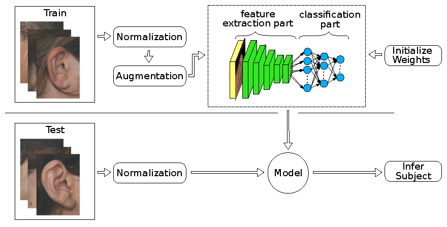
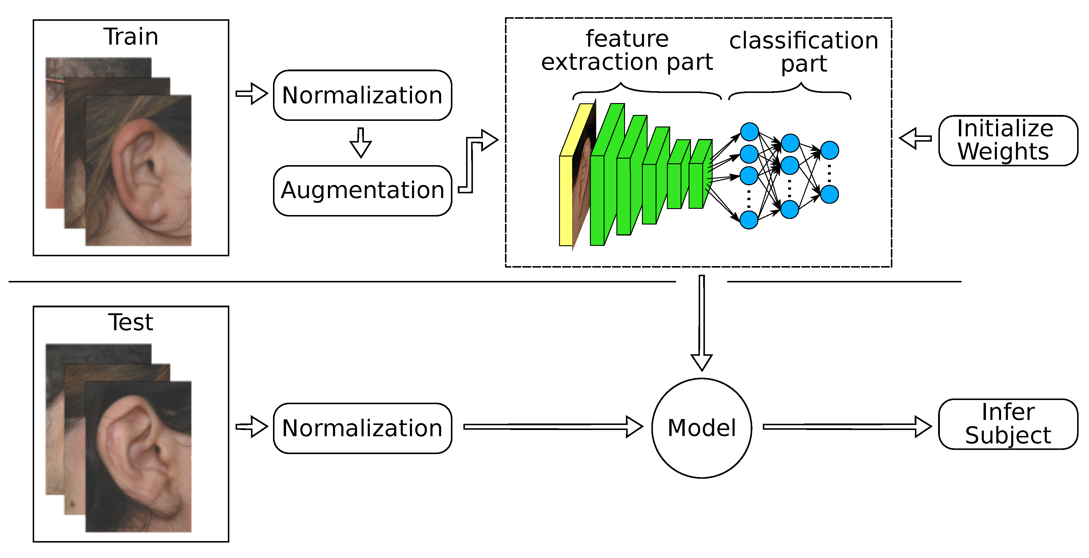
As the present datasets contain only up to 804 images, over-fitting was expected to affect the training process. Even with elaborated data augmentation, it is difficult to achieve decent accuracies. In the feature extraction strategy, this issue is completely circumvented by using pretrained models on ImageNet [
6] as fixed feature extractors. We divided the network into a convolutional feature extraction part and a fully connected classification part, as shown in
Figure 2. Since AlexNet is composed of a convolutional feature extraction block of five convolutional layers and a classification network on top with three fully connected layers, we froze all convolutional weights because their filters might be generic enough for being transferred to similar recognition problems as reported in [
57,
58]. We replaced the fully connected layers with new layers, where each of the first two layers had 2048 neurons, and a final layer with a softmax classifier that had neurons equivalent to the number of subjects in each ear dataset. We used linear Kaiming initialization [
56] to initialize the newly added layers. During the training process, we adjusted only the three fully connected layers and their batch normalization layers until convergence.
4.5. Feature Extraction + Batch Normalization
We also considered a slight variation of the feature extraction strategy, where batch normalization was applied only before each fully connected layer. To investigate the level of genericness of the ImageNet features, we included batch normalization in the convolutional part and thereby lowered the risk of having low performance due to normalization issues. This strategy is called feature extraction + batch normalization (feature extraction + BN). Hence, in this learning strategy, we applied batch normalization before each layer, which included the convolutional ones. Only the fully connected layers and all batch normalization layers were trained under this strategy.
4.6. Fine Tuning
Using the pretrained models as feature extractors is usually a first approach for transfer learning. A more effective way of transferring the learned representations is to fine tune the entire pretrained model on the new recognition task. When performing fine tuning, the network weights of the convolutional part are initialized from the pretrained ImageNet model, while the new fully connected layers are initialized in a similar manner to the feature extraction strategies. We then performed domain adaptation or retraining the entire network with the limited ear images from the training set until convergence.
5. Experiments and Results
In order to explore and compare the recognition performance of handcrafted and CNN features, we selected seven top performing manually designed features and evaluated their performance against four types of CNN features obtained from an AlexNet-like architecture. We report the results on three ear datasets, which contain an increasing level of image variations reflecting constrained and unconstrained (in the wild) imaging conditions.
We first provide a brief description of the ear datasets and then discuss our data augmentation techniques to increase the number of training examples during training and fine tuning the deep models. Subsequently, the experimental setup for both handcrafted features and deep models is presented. Finally, the obtained results of our experiments are discussed, and visualizations of the features are performed and analyzed.
5.1. Ear Datasets
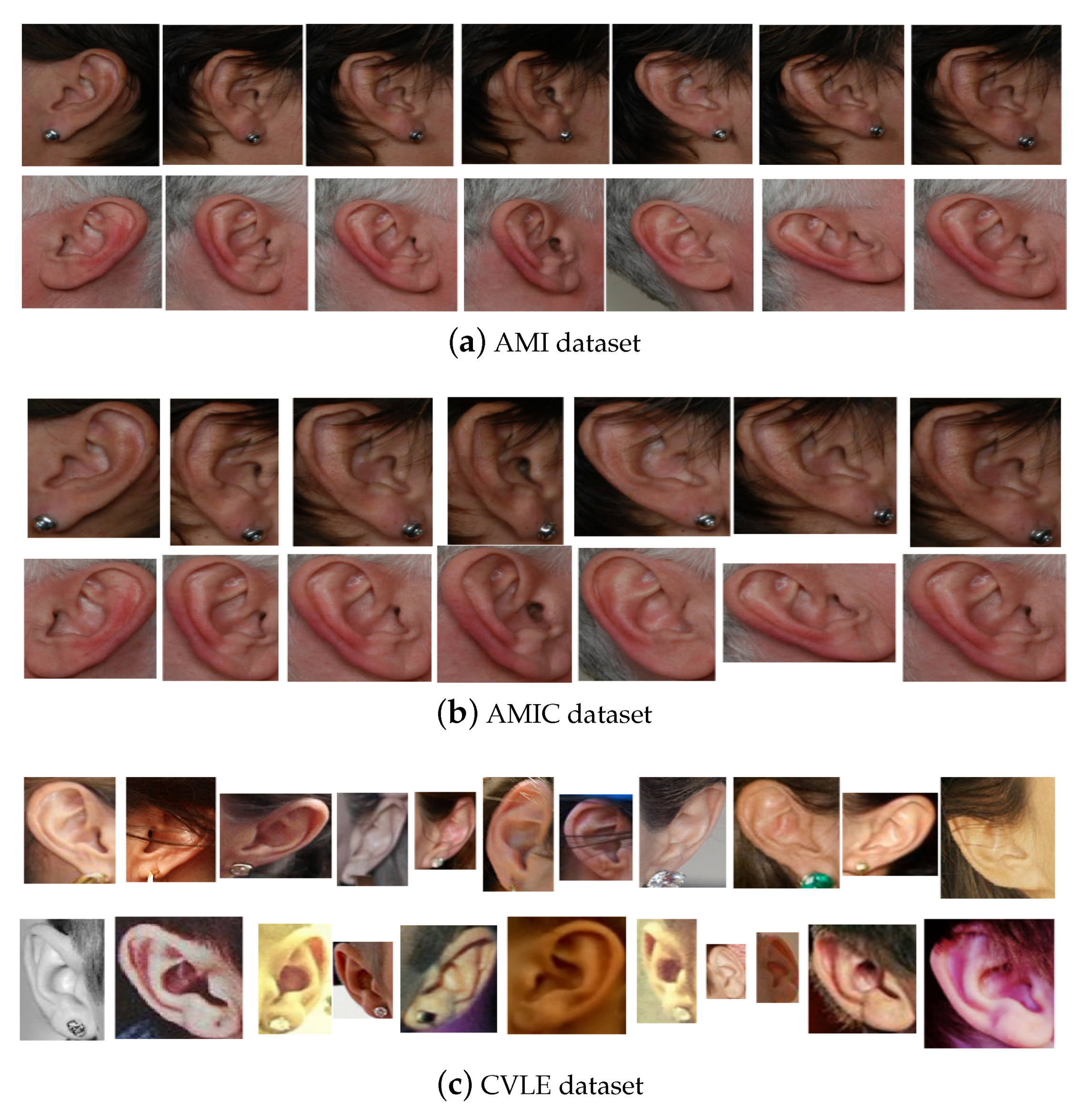
The first dataset was the Mathematical Analysis of Images (AMI) ear database [
59]. It contains 700 ear images acquired from 100 subjects. The images were acquired for the right and left ears from both males and females. Each subject had seven images, six for the right ear and one for the left. All images were taken by the same source camera under similar lighting conditions. The images were captured for the subjects with various poses like looking forward, up, down, left, and right. Furthermore, one image was acquired under different scales. The images had a spatial resolution of
pixels and were in JPEG format.
Figure 3a shows sample images for two subjects from the AMI dataset.
The second dataset was the AMIC, which is a cropped version of the AMI dataset introduced in [
14]. It contains the same number of subjects and images, but after removing any unwanted background such as hair and neck parts from the profile images. Cropping also helps to make the geometric ear structure and shape visible to feature extraction methods and obtain their representations based on the distinguishing ear characteristic features, but this makes it more challenging. As a result of manually cropping the AMI ear images, all images in AMIC dataset have variable sized spatial resolution ranging from
pixels to
pixels.
Figure 3b illustrates the cropped images for the same two subjects shown in
Figure 3a.
The third dataset was the Computer Vision Laboratory Ear (CVLE) database introduced in [
60]. It contains 804 ear images of 16 individuals where an individual had between 19 and 94 images. All images were collected from the web for both genders of different ethnicities. The images were taken with different cameras and under different indoor and outdoor lighting conditions. The subjects were photographed with different viewing angles between
to
and beyond. The images had variable spatial resolution starting from
pixels and under
pixels. The images were also occluded by hair and accessories like earrings and headphones and exhibited different contrast. These image conditions represented the unconstrained or in the wild image settings. Example images showing these variations present in the CVLE dataset, for two subjects, are shown in
Figure 3c.
5.2. Data Augmentation
Training deep models with millions of parameters requires large scale datasets. In realistic settings of ear recognition scenarios, the small amount of images does not leverage the large variability of the dataset and the conditions under which the images have been taken. One effective solution for addressing these limitations is to augment the existing training dataset by producing variants of the same image through a pre-defined set of domain specific image transformations. Therefore, in order to improve the robustness of the obtained models against a wide range of image variability, we showed transformed images to the deep network. The synthetically generated samples added to the training data and introduced some changes that enhanced the learning ability of the models and made them robust against such variations. Since only limited amount of ear images was available for training, different data augmentation techniques were performed in order to avoid over-fitting and enhance the generalization ability of the models.
In our experiments, we combined several image manipulation operations into a comprehensive augmentation pipeline, which was applied on the fly for each training image in every epoch. In order to handle datasets with different aspect ratios, we randomly scaled the image to fit into a pre-defined canvas. Subsequently, we rotated the image randomly and performed horizontal shearing. After that, random cropping was performed while keeping the aspect ratio. After resizing the image to the fixed canvas size, we further augmented the image using Gaussian blur, adding Gaussian noise, introducing random changes of brightness, contrast, saturation, and hue. Finally, we applied a 50% chance of flipping the image horizontally. The augmentation steps were performed on each training image in each epoch in order to drastically increase the amount of training samples. We performed the data augmentation on the CPU, and we did it in parallel with the network training on the GPU to reduce computation time. Nevertheless, we found that preprocessing the images was a computational bottleneck because it involved loading a large number of files and a long chain of serial augmentation steps. However, it is worth mentioning that without augmenting the training sets, the obtained models were susceptible to substantial over-fitting.
5.3. Experimental Setup
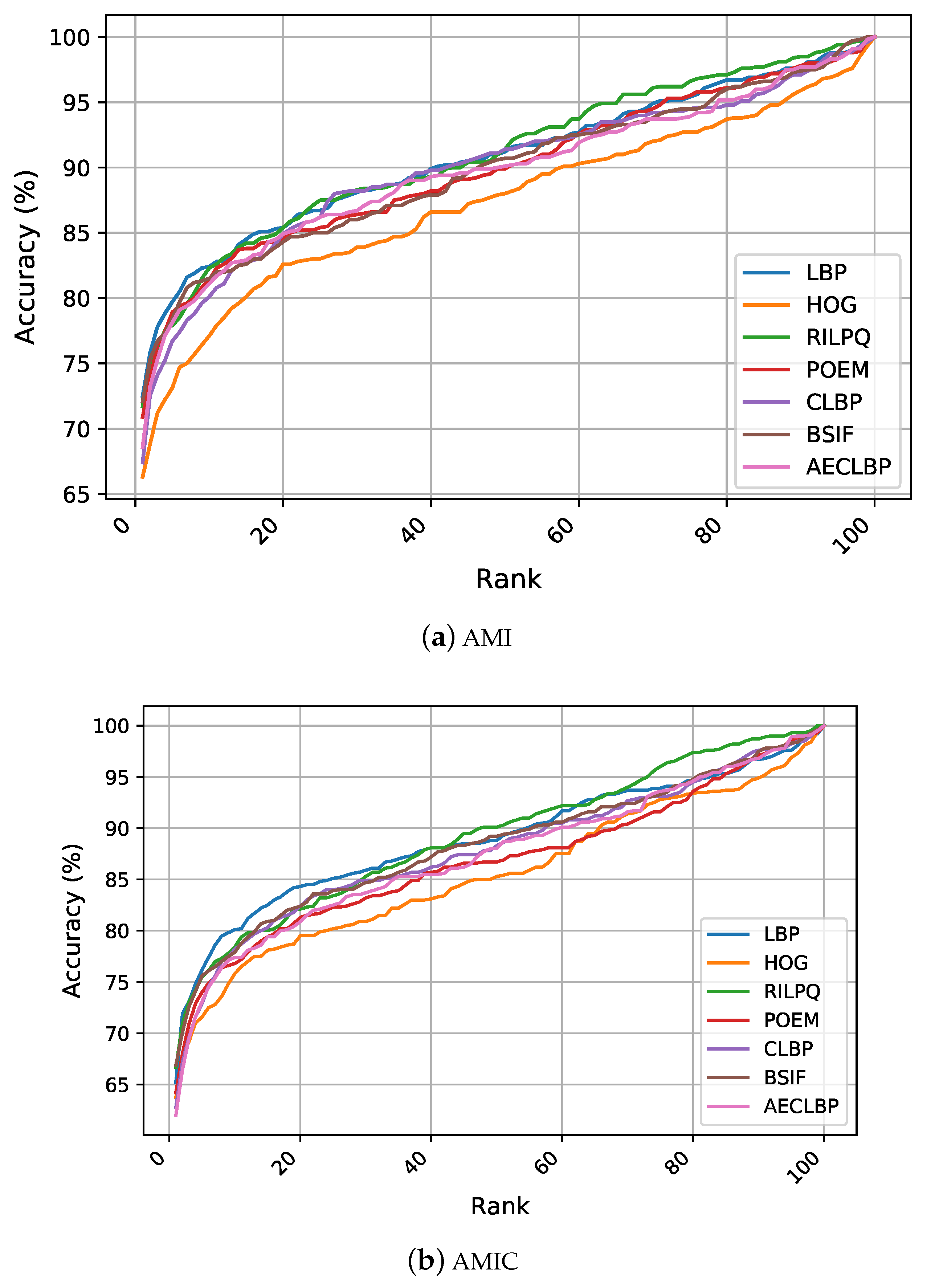
The experimental protocol followed in this work to evaluate the recognition performance of handcrafted and CNN features was five-fold cross-validation. The results are reported with the mean and standard deviation over the five folds. The Cumulative Match Characteristic (CMC) curves for each recognition experiment on each dataset are also visualized. Besides, three quantitative evaluation metrics of Rank-1 (R1) and Rank-5 (R5) recognition rates and the Area Under the CMC (AUC) are provided.
For increased comparability, the handcrafted features shared a unified recognition pipeline to obtain the final results similar to the setup mentioned in [
22,
41]. The input ear images underwent several phases including, preprocessing, feature extraction, classification, and finally visualizing the results. As preprocessing steps, images were converted into gray scale images, resized to
pixels, and enhanced by applying the histogram equalization technique. Then, the preprocessed images were subjected to the feature extraction phase where the underlying descriptor extracted relevant image characteristics. The output of this phase was an image specific feature vector representing the characteristics of the ear image. Subsequently, the feature vectors were used to train linear SVMs for classification in a one-vs.-rest approach. The last phase comprised computing the performance metrics and plotting the CMC curves for visualization of the overall performance. The implementation details and hyperparameters values of the considered feature descriptors are given in
Table 2.
When training and fine tuning deep models, we used a slightly different experimental setup as the feature extraction step and the classification step were combined. For feature extraction (with and without) batch normalization and fine tuning, we exploited pretrained models trained on the ImageNet dataset [
6] with 1000 classes and performed adjustments on some layers to shrink down the architecture and suit the number of classes in each ear dataset. We changed the architecture to suit the ear recognition problem as described in
Section 4.
In order to consider the variable image sizes in each dataset, we placed the images into a canvas of size of
pixels for the AMI and AMIC, while for the CVLE dataset, we found the optimal size to be
pixels, thereby keeping their aspect ratios. To investigate the effect of spatial resolution on the recognition accuracy, we performed the experiments with different canvas sizes. We chose the minimal canvas size for which the drop of the Rank-1 recognition rate was still insignificant and under
. We performed extensive data augmentation as described in
Section 5.2.
On the AMI and AMIC datasets, training from scratch needed 600 epochs for convergence, and the learning rate was divided by five after 200 and 400 epochs. However, the CVLE dataset to require different sets of hyperparameters and training from scratch needed more epochs with 900 iterations, and we divided the learning rate by five after 300 and 600 epochs. The feature extraction strategy converged after 450 epochs, and we reduced the learning rate at 150 and 300 epochs. For the fine tuning strategy on AMI and AMIC, the training converged after 150 epochs, and the learning rate was scheduled to be divided by five after 50 and 100 epochs, respectively, whereas when fine tuning on the CVLE, we trained for 300 epochs and reduced the learning rate after 100 and 200 epochs. For all the mentioned strategies, we started by an initial learning rate of 0.02 and used a batch size of 50. The networks were trained on a PC with Intel(R) Core(TM) i7-3770 CPU, 8 MB RAM and Nvidia GTX 1080 using stochastic gradient descent and the cross-entropy loss. We regularized training with dropout and a momentum of 0.8 to alleviate over-fitting.
5.4. Results and Discussion
This section reports the experimental results for both handcrafted and CNN features. The obtained results are summarized in
Table 3 using performance metrics of R1, R5, and AUC. The relevant work from the literature was also included for a direct comparison. To explore the comparability across the different methods, the CMC curves are presented for each recognition experiment in
Figure 4 and
Figure 5. We started our analysis by interpreting the recognition performance of the handcrafted features, then continued with the CNN features.
5.4.1. Handcrafted Features
Our recognition experiments target evaluating and comparing the discriminative powers of the feature extraction methods in describing ear images for recognition using an SVM. The recognition results in
Section 5.4 indicate the superior performance of the LBP descriptor over all other traditional methods on the AMI dataset with R1 recognition rate of
. On the AMIC and CVLE datasets, BSIF was the top performer with mean recognition rates of
an
, respectively. Additionally, the AMIC dataset, which is the cropped version of AMI, reached significantly lower accuracies than its uncropped counterpart. This indicated the benefits from the extra parts of profile images when encoding ear images and showed that conventional feature extractors and traditional classifiers made use of hair and skin to increase performance.
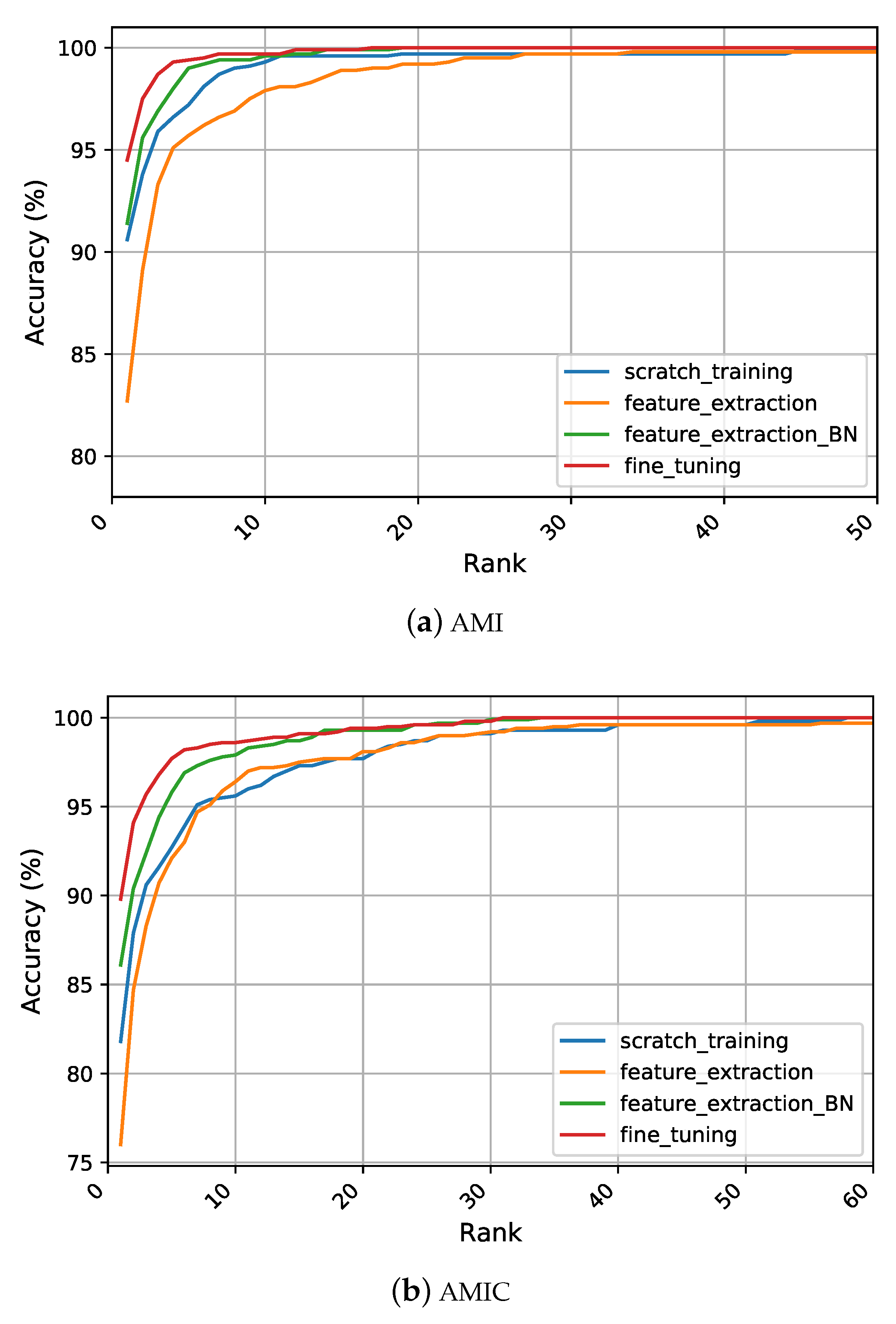
Figure 3 illustrates the CMC curves, which summarize the performance on the considered ear datasets. Considering the AMI and AMIC datasets, LBP and RILPQ obtained approximately similar performance with slight improvement over other features. Despite the diversity of image variations introduced under the unconstrained conditions reflected in the CVLE dataset, the conventional features achieved higher recognition rates compared to AMI and AMIC datasets due to having less subjects and more images per subject. Although the performance differences among all competing manual descriptors were relatively small, the CMC curves showed noticeable improvements for the gradient based descriptors BSIF, HOG, and POEM compared to the texture encoding methods of LBP, CLBP, and AECLBP.
Even though the reported results in our experiments were based on the entire ear images from each dataset for a fair comparison between the considered features, it is worth mentioning that the conduced experiments assumed bilateral symmetry between left and right ears. However, when we conducted the experiments on the AMI and AMIC datasets using 600 ear images for the right side only, an improvement between
and
was achieved in recognition performance. The R1 recognition rate for LBP rose from
to
, and the highest R1 rate was achieved by CLBP at
on the AMI dataset. For the AMIC, the R1 recognition rate for BSIF rose from
to
, and the highest recognition performance was obtained by RILPQ with R1 of
. These obtained results indicated that the left and right ears shared some degree of symmetry, while not being identical. The reader is referred to [
63] for a detailed study on the anatomically symmetric and asymmetric substructures of the ears.
5.4.2. Scratch Training
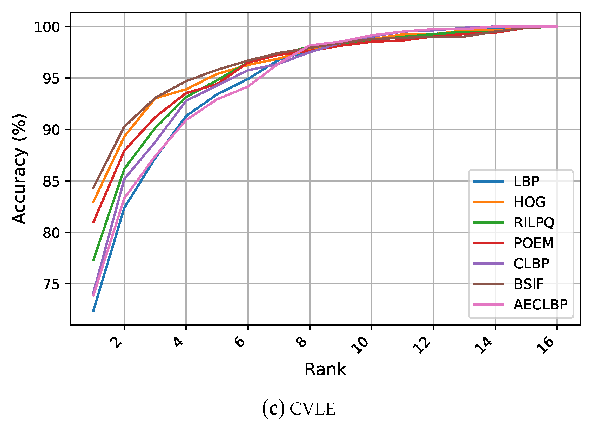
Figure 5 summarizes the differences in recognition performance under each representation learning strategy on the considered datasets. When training the network from scratch on the AMI and AMIC dataset, significant improvements in the recognition rates were achieved compared to the handcrafted features as reported in
Section 5.4. On the AMI dataset, an R1 recognition rate above
was achieved, which was
higher than the best performing texture descriptor, i.e., LBP. Furthermore, we report a significant improvement for the other evaluation metrics of R5 and AUC indicating the continuous learning of more discriminative features by the models. Despite the drop in all metrics when using the AMIC dataset, still, the learned features achieved better performance than handcrafted features with a large margin of at least
over the top traditional performer. The reason behind the success of the learned features was their ability to learn complex and more discriminative patterns from images such as edges, corners, and textures, while handcrafted features were specifically designed to encode certain characteristics of the given images. Thus, the subsequent classification technique was limited in the predetermined representation and could not leverage other important features that were useful for distinguishing between the individuals as well. Furthermore, since handcrafted representations are usually ad-hoc and specific, they were incapable of being generalized to deal with various realistic scenarios. However, the BSIF descriptor still gave better results than the scratch training strategy on the CVLE dataset. One logical reason for the success of the BSIF is its nature in computing the binary code, which depends on a set of learned filters rather than manually predetermined filters. Another possible reason for this observation was given by the huge intra-class variance within CVLE, which could not be easily taught to a CNN with the few images it contained.
5.4.3. Feature Extraction
The second learning strategy involved transfer learning using a pretrained AlexNet network with weights learned on the ImageNet dataset. We froze the convolutional part of the network and used it as a fixed feature extractor. As can be seen in
Section 5.4 and
Figure 5, the results were lower than training from scratch. However, these features still achieved a performance gain of
over the best handcrafted features. The results from this learning strategy justified that the pretrained CNN was capable of performing feature extraction better than any handcrafted feature descriptor on both AMI and AMIC datasets. For the CVLE, the extracted features achieved an R1 of
, which was still higher than the LBP features and their variants of CLBP and AECLBP features. Even though, on first glance, it seemed that the extracted features from the ImageNet model did not suit the ear recognition problem well. However, the discussion is continued in the following learning strategy.
5.4.4. Feature Extraction + BN
In an attempt to understand the drop in performance when allowing only the classification part to be adjusted during training, we observed that adding batch normalization layers after the activation functions yielded improved recognition rates for all datasets. More specifically, when training the seven batch normalization layers along with the fully connected layers, this led to an improvement over the feature extraction strategy by a margin of about
for AMI,
for AMIC, and
for CVLE. For AMI and AMIC, this training strategy performed even better than training from scratch. Improving the recognition performance by adding batch normalization means in general that using CNNs as feature extractors can be bound to normalization problems. Here, normalization was conducted with the mean pixel and standard deviation of the ImageNet database, which is a common choice. However, this normalization step did not seem to be enough to attain good results for the second training strategy feature extraction. By only learning the eight additional parameters of four batch normalization operations, an improved recognition performance with an R1 of
was achieved using the AMIC dataset, which was only about
less than for the top performing fine tuning strategy discussed below. Considering the CMC curves in
Figure 5, we observed the supremacy of feature extraction combined with batch normalization over using either scratch training or feature extraction on all datasets.
5.4.5. Fine Tuning
Instead of only training the classification part of the deep network and its batch normalization parameters, we adjusted all parameters of the network to the ear recognition problem. This strategy resulted in the best performance among all considered CNN features. Fine tuning the pretrained model achieved an R1 of
for the AMI dataset, which was
higher than the best performing handcrafted feature descriptor. These results made fine tuning deep CNNs the new state-of-the-art method to solve the ear recognition problem on the AMI dataset. Consistent with the other training strategies, the AMIC dataset proved to be more challenging than the AMI dataset. Nevertheless, fine tuning gave the best results among all four training strategies and achieved a high accuracy with an R1 of
. With the fine tuning strategy, the previous top performing hand-engineered feature BSIF could be superseded by a margin of about
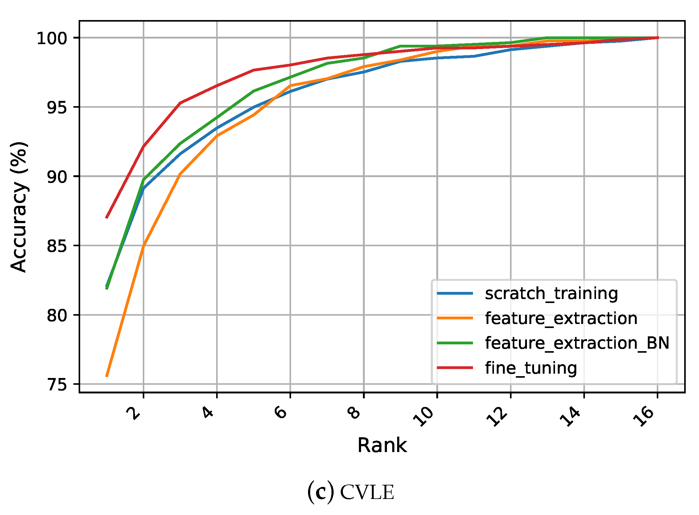
on the challenging CVLE dataset. Out of the four strategies, fine tuning proved to be the most effective, as can be clearly observed from the CMC plots shown in
Figure 5.
5.5. Visualization of Handcrafted and CNN Features Using t-SNE
After showing the superiority of the CNN features over the seven handcrafted ones on the given datasets, it is desirable to find a meaningful explanation for this finding. Here, visualizations of the different features are performed using t-SNE [
21], which is a non-linear dimensionality reduction technique. It maps multivariate data on 2D or 3D space in an unsupervised manner. It also allows exploring and visualizing the data by maintaining relationships and preserving its local structure.
We started by extracting both handcrafted and CNN features from the CVLE ear dataset. The features were mapped onto a 2D space using t-SNE visualization in order to learn about their differences. However, the visualization was non-deterministic and t-SNE was applied multiple times with different parameters in order to ensure consistency. Especially the perplexity parameter, which sets the effective number of neighbors, had a significant impact on the mapping. At the end, three visualizations were manually selected to be shown in order to present the most dominant structure within the data. We did not show t-SNE visualizations on the AMI and AMIC datasets because the number of samples per class was too low to analyze how the individuals clustered qualitatively. This was why we focused on the CVLE dataset, which had more samples per class and was visually easier to interpret.
First, the best performing handcrafted feature was visualized. The feature vectors were extracted using the BSIF descriptor for all images in the dataset. Subsequently, t-SNE visualization was performed. The Manhattan distance was used as a distance metric because it is widely used for histogram data. However, the visualizations did not really change qualitatively when using the Euclidean distance. Second, in order to compare the handcrafted features to the CNN features, an AlexNet based model that was pretrained on the ImageNet database was used as a feature extractor. The input images were normalized according to the ImageNet dataset and propagated through the network. The input to the last fully connected layer was used as a feature vector. The Euclidean distance was used for the t-SNE algorithm because other distance metrics did not lead to better clustering of the individuals. Third, to investigate the features of the network, which were fine tuned on the particular ear dataset, the test set was propagated through the network, and the feature vectors were extracted. Again, the Euclidean distance was used for the t-SNE algorithm. We also applied the t-SNE algorithm on the output of the last convolutional layer of the fine tuned model. However, no clustering of the individuals could be observed as these feature vectors turned out to be too generic for distinguishing the individuals.
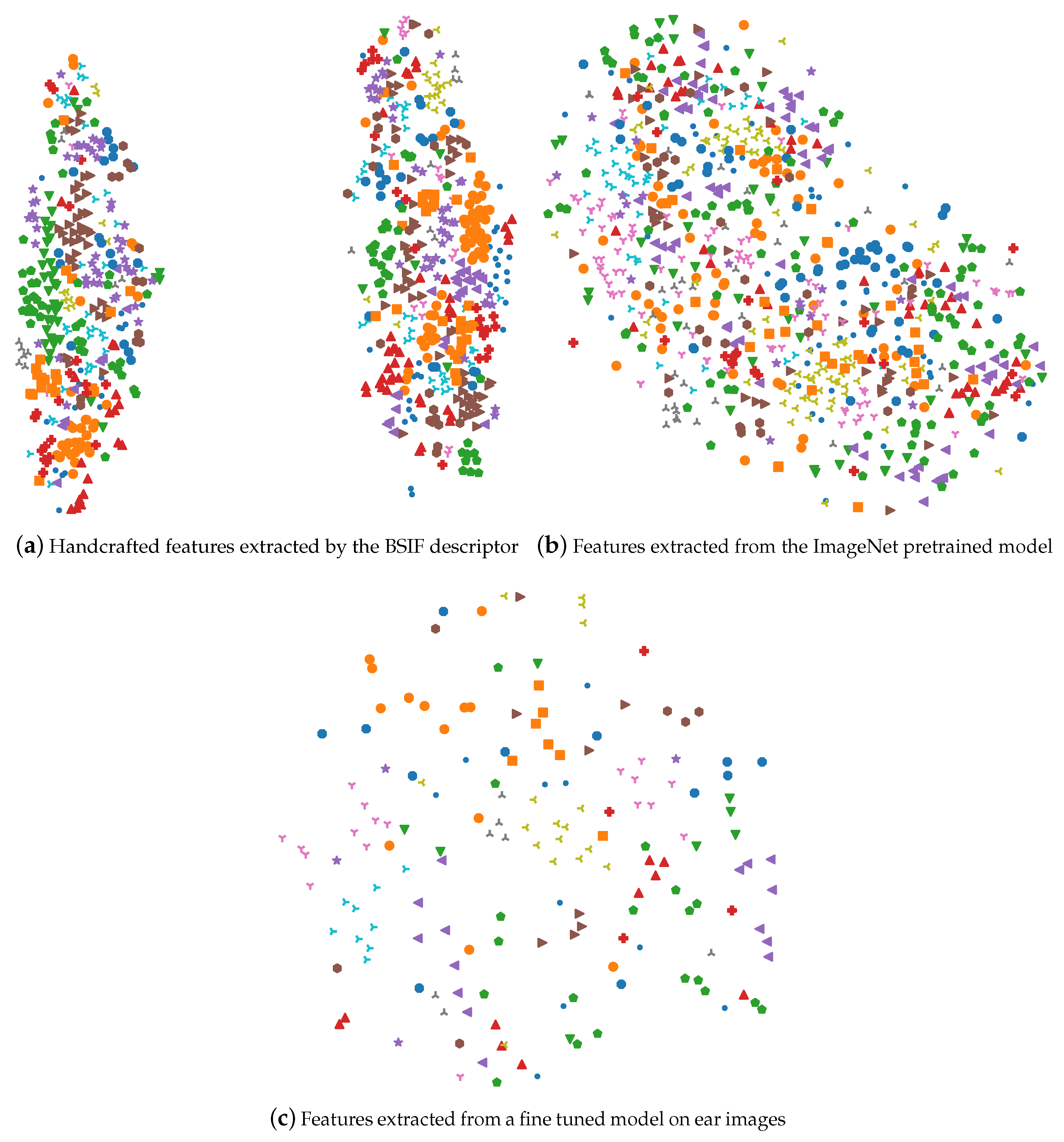
Figure 6 illustrates the feature visualization for the CVLE ear dataset. The diagrams showed the two-dimensional map of the multivariate feature vectors. Each symbol represented a unique individual. Symbols across different visualizations might not correspond to each other. To avoid clutter and to improve the readability of the diagrams, the number of subjects was limited to 40. Usually, the samples from one individual were spread across several small clusters. As observed in
Figure 6a, the handcrafted features consistently formed two global clusters, which even occurred among a wide range of perplexity values. This observation applied to all datasets, though it was only shown for the CVLE dataset. The two clusters refer to the image displaying the right or the left ear, which can be concluded from counting the number of instances per individual. This made sense for the handcrafted features, because the left ear and the right ear had different dominating gradient directions, which led to different histogram characteristics. Thus, feature vectors of the opposite ear were very dissimilar and were not likely to be neighbors. Consequently, the t-SNE algorithm placed them far away from each other.
The features that were extracted from the ImageNet model showed a similar phenomenon, but far less pronounced, as shown in
Figure 6b. The two clusters showed up; however, they were somehow connected, and no perplexity could be found where the two clusters showed up as clearly as for the handcrafted features. However, the fine tuned model did not show this behavior (
Figure 6c), due to the learning process and the insight from the profound data augmentation during fine tuning. Flipping the images horizontally was one step in the image transformation pipeline and enhanced the model generalization as it gave the model a chance to treat both left and right ears in the same way. Moreover, fine tuning the network on the ear dataset considerably reduced the variance between the right and left ear.
6. Conclusions
This paper presented several ear recognition models built using conventional descriptor-classifier and deep learning based approaches. Experiments were conducted to compare the performance of seven state-of-the-art handcrafted features and four types of CNN features extracted from a variant of AlexNet. The features were investigated in their robustness to represent ear images acquired under controlled and uncontrolled settings from three datasets.
The obtained results indicated that CNN features were superior in recognition accuracy, outperforming all handcrafted features. The performance gain in recognition rates was above over the best performing descriptor on the AMI and AMIC datasets, where the number of images per subjects was relatively small. However, the performance gain was within for the CVLE dataset, which had fewer subjects and more images per subject, but higher intra-class variability.
In order to find logical and meaningful interpretations for the superiority of the CNN features, we applied t-SNE visualization and mapped the extracted features onto a 2D space to explore their internal structure. We observed that handcrafted features consistently formed two clusters representing the right and left ear, respectively. The feature vectors of the opposite ear were found to be very dissimilar, and therefore, t-SNE visualization placed them far away. However, the feature vectors extracted by the fine tuned model did not show this behavior, which indicated a better adaptation to the ear data during the fine tuning process. The features of the fine tuned network turned out to be invariant to the side of the ear and thus were more suitable for the present ear datasets.
To summarize, our main conclusions from the ear recognition experiments conducted here were:
CNN features were superior to handcrafted features, which was consistent with the relative performance of deep CNNs in other image recognition tasks.
CNN features were invariant to choosing the left or the right ear, while traditional descriptors were severely affected.
For handcrafted features, we noticed an improvement between
and
in recognition performance on the AMI and AMIC datasets when conducting the experiments using ear images from the same side. That means the left and right ears shared similar features, but were not ideally symmetric. These findings also matched the reported results from [
3,
64,
65], which indicated a noticeable drop in recognition accuracy when training on ear images from one side and testing on ear images from the other side. That means for some individuals, the left and right ears did not share the exact shape and a certain degree of asymmetry did exist.
Using pretrained models as feature extractors on new data or for a new recognition task was not sufficient due to the difference between the learned features for the different tasks. However, adapting or fine tuning the pretrained model on new data related to the target task led to significant improvements in performance. The models fine tuned on each ear dataset consistently performed best.
Batch normalization was crucial when using pretrained CNNs as feature extractors on new data. We recommend adjusting the mean and the standard deviation of batch normalization layers.
Since no recognition experiments were conducted on the AMIC dataset using handcrafted descriptors in the literature, we carried out recognition experiments to investigate the impact of removing the auxiliary background parts. We observed that both handcrafted and CNN features were affected by the cropping of AMI images to a similar degree with a superior performance of CNN features at .
Even though our main objectives in this study were to show that CNNs can be trained using small datasets, it is possible to improve the performance further when more training data is available to learn more specific ear features and when top performing and state-of-the-art CNN architectures are employed. Therefore, our future work will include large scale ear datasets with a wider range of image variations and more subjects. Moreover, we will also consider more recent CNN architectures such as Inception [
66,
67,
68], ResNet [
69], SqueezeNet [
70], ResNeXt [
71], DenseNet [
72], and MobileNet [
73], and explore different learning strategies. Of the same interest is to explore different combinations between handcrafted and learned features to further improve the recognition accuracy. Another interesting research direction is extending our study to include other visualization techniques to enhance our understanding of the decisions behind the models’ predictions.


