Efficient Vanishing Point Detection for Driving Assistance Based on Visual Saliency Map and Image Segmentation from a Vehicle Black-Box Camera

Abstract

Techniques for detecting a vanishing point (VP) which estimates the direction of a vehicle by analyzing its relationship with surrounding objects have gained considerable attention recently. VPs can be used to support safe vehicle driving in areas such as for autonomous driving, lane-departure avoidance, distance estimation, and road-area detection, by detecting points in which parallel extension lines of objects are concentrated at a single point in a 3D space. In this paper, we proposed a method of detecting the VP in real time for applications to intelligent safe-driving support systems. In order to support safe driving of autonomous vehicles, it is necessary to drive the vehicle with the VP in center of the road image in order to prevent the vehicle from moving out of the road area while driving. Accordingly, in order to detect the VP in the road image, a method of detecting a point where straight lines intersect in an area where edge directional feature information is concentrated is required. The visual attention model and image segmentation process are applied to quickly identify candidate VPs in the area where the edge directional feature-information is concentrated and the intensity contrast difference is large. In the proposed method, VPs are detected by analyzing the edges, visual-attention regions, linear components using the Hough transform, and image segmentation results in an input image. Our experimental results have shown that the proposed method could be applied to safe-driving support systems.

1. Introduction

The development of autonomous vehicles is aimed at effecting fundamental changes in vehicle use, so that, through use of autonomous vehicles, it is hoped that benefits such as prevention of traffic accidents, additional free-time, and pollution reduction can be achieved. For successful autonomous driving, estimating optimal driving information is necessary, using various sensors such as infrared, radar, vision, thermal image, and Global Positioning System (GPS), among others. Globally, automobile manufacturers have recently been investing in automotive information technology and the development of technology for autonomous vehicle deployment [1,2,3,4,5]. The key technologies that are applied in autonomous vehicles include recognition of the driving environment on behalf of the driver, detection of the vehicle position during driving, detection and recognition of objects on the road (such as other vehicles or pedestrians), and implementation of devices and components required for vehicle steering. Currently, advanced driver-assistance system (ADAS) technologies are the subject of continuous study, and have been developed to recognize information relating to various surroundings and objects on the road [6,7,8,9]. ADAS technology is one of the key technologies in autonomous vehicles for lane, road, vehicle, pedestrian, traffic light, and obstacle recognition. In particular, in analyzing the driving situation of vehicles, assisting the driver, determining distances to other moving vehicles, determining the motion direction of vehicles, and determining vehicle position in a lane are important. To obtain such information, vehicle location and motion-direction information is used, and expensive additional devices such as an infrared ray system, an ultrasonic wave system, radar, and a stereo camera need to be used for its acquisition. These devices are installed at the lower part of the front portion of the vehicle, making it possible that they would be incapacitated, or would need to be replaced, in cases of a minor contact accident which can result in increased damage. In recent years, the use of vehicle image-recording devices has grown rapidly, however, these devices are only used for determining responsibility after an accident. Information can be provided to a driver in advance through an image-processing algorithm [10,11,12], however, interpreting three-dimensional (3D) structural information on the surroundings in which a vehicle is located by simply acquiring a two-dimensional (2D) image from the vehicle image-recording systems, such as a vehicle black box, can be challenging. Consequently, a method is needed that can develop 3D vehicle position information from a 2D image. Vanishing point (VP) detection technology has been applied to 2D and 3D images in several studies [13,14,15,16,17,18,19,20], to estimate objects, distances, camera parameters, 3D positions, depths, and the areas of objects of interest. The VP is used to reconstruct 3D objects, and the method that detects the VP of an image involves connecting adjacent feature information such as edges to draw a straight line, and to project the extension line in the image by selecting an intersection point. In other words, VP estimates using the symmetrical features of the surrounding structure in the image. There is a feature detection method to detect the vanishing point. In the feature detection method, the intersection of line segments is detected by analyzing the linear connection components between the features included in the image. Hough transform is used to detect the linear component of feature information in the image [21,22,23].

In general, images are required so that extraction of meaningful feature information using irregular feature information caused by noise, uneven illumination, and color changes due to brightness discontinuity can proceed. Finding straight-line components connected to one another in the extracted meaningful feature information is possible by applying the Hough transform process. However, in an urban road environment with complicated background features, numerous straight-line segments can be detected, so that, to detect the actual VP, additional processing elements such as the number of lines, angles, and brightness threshold values are required.

Barnard [24] used a Gaussian sphere to detect VPs, and accumulated the extensions of all the straight lines in a plane image in a Gaussian sphere. The accumulated values included the local maxima of the horizontal and vertical axes of the branch chosen as the VP, however, the difficulty with this method was that calculating the possibility of a straight line with respect to all pixels, and a plurality of local maximum values existed, which necessitated an additional processing step to select the VP.

Kong et al. [25] used directional information from an image texture to detect the VP. Eight disjointed components with similar directions were detected in the image, including the point where most straight-line intersections occurred. A Gabor wavelet filter was applied to extract text directional information (five scales, 36 orientations), and converted each pixel of the input image into directional information. The local adaptive soft-voting method was then used iteratively, to calculate the information change rate between the directional information pixel and all other pixels. A VP was then selected, based on the connected candidate feature information showing a small rate of change. The real-time processing requirements necessary for application in autonomous vehicles was the disadvantage with this method, calculating the texture change rate for all pixels, in the 36 texture direction images in the five-step reduced image, could be too time consuming.

Suttorp and Bucher [26] repeatedly selected a candidate VP by applying a line segmentation-based filtering method, and chose a pixel with the maximum accumulated selection value as the VP. Although this method presented the advantage of being applicable to different environments, it suffered limitations in the context of real-time applications for autonomous driving, due to the use of iterative algorithms. Based on these issues, most VP detection studies first select the candidate VPs in the image. To select an optimal candidate point among all other points, the VP is estimated by repeatedly applying low-level feature information from the image. To detect the optimal candidate VP, the methods considered so far suffer from limitations in real-time applications such as in autonomous vehicles due to long execution time they need to apply iterative algorithms, such as the expectation and maximization algorithm.

Ebarhimpour et al. [21] proposed a method for detecting straight lines using the Hough transform and the K-means clustering algorithm on visual-information from an input image, to reduce the execution time in detecting the VP. The proposed method was effective in checking straight-line components with a 45° angle, which represent formal structures such as an indoor corridor. However, there was again the disadvantage that computation time, in this case for the K-means clustering algorithm, was large.

Choi and Kim [27] proposed a dynamic programming method using a block-based histogram of oriented gradient to reduce complex computation time and proposed an efficient VP detection method. Its disadvantages included poor accuracy of the input image, as the method was applied to pixel-based region segmentation, such as road-boundary selection, in the detection of a disappearing block, based on a 32 × 32 block unit. Consequently, real-time processing and accurate detection were required so that the VP acquisition in the image obtained from the video-recording device installed in the running vehicle could be applied to the vehicle.

In the VP detection of the previous research [28], three directional text information (0, 45, 135) was used, and the processing time averaged 1.475 s except for the image analysis step. In addition, the accuracy of VP detection in [28] is about 82%. In addition, the experiment was conducted only in the highway environment, and there is a problem of low VP detection rate in the actual road environment.

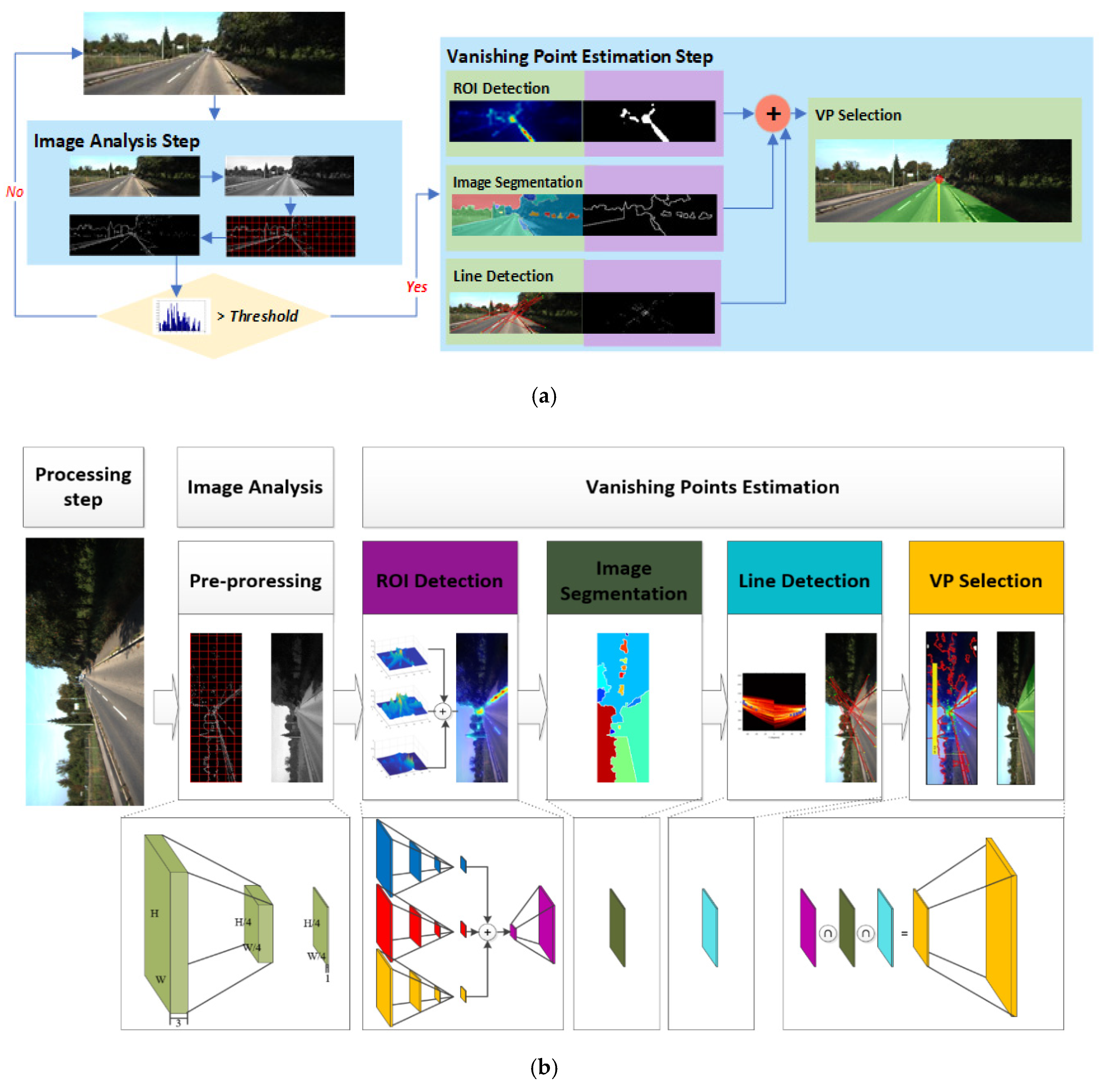
Considering all the issues mentioned above, we have proposed here a method that uses visual-attention area detection and Hough transformation of the edges, based on directional feature information, to detect the VP of a road image in real time. As mentioned earlier, to detect the VP, straight line and other directional information must be extracted from the feature information of the image, however, feature information and linear component extraction from all input image pixels suffers from the imposition if excessive real-time processing, due to increased calculation times. In addition, whereas existing feature voting methods can detect accurate VPs, they cannot be applied to real-time information such as road-driving situations. In our proposed method, the VP is determined by selecting candidate VP regions, and the Hough peak point is then selected using the Hough transform, to derive the fast-linear components, so that the position where at least two straight-line components intersect is then determined as the candidate VP. The point with the maximum value is then identified as the VP, by comparing the edges of the visual-attention regions (VRs), including the candidate VPs with texture directional feature information.

Definition of VP Location and Problems

A VP is a point that concentrated in one place on the 2D image plane while projecting lines parallel of each other in 3D space. In general, a VP is a point on the horizon, a place that is structurally concentrated in a 3D environment [29]. For example, a VP can be chosen as the point where a road meets the sky, or where a vertically parallel road lane and a road boundary structure meet. However, because of complicated road environments, road imaging needs complete 3D structure analysis, which requires considerable processing.

In general, image segmentation is a method for determining a location where a road area and a sky area meet each other. The vanishing point is a point where feature information is concentrated in an image, and in order to detect it effectively, it is necessary to select a place where feature information is collected the most. Therefore, a process of using a visual saliency model to detect where feature information is concentrated in a road image and detecting intersections of straight lines through a Hough transformation is required.

The proposed method proposes a method to detect vanishing points that combine image segmentation results, visual attention area detection results, and intersection point results of straight lines to detect vanishing points in road images. In this paper, we have proposed an effective method for VP detection on road images. First, a video-recording device was installed in a vehicle, at driver eye-level and horizontally relative to the road, in such a position that left–right and up–down slopes could be assumed to be zero.

In our method, the location of the VP in the image obtained from the black-box camera installed in the vehicle is defined in

Table 1. Definition of vanishing point (VP) location in a road environment based on the proposed method.

Coordinates must be located where much feature information is concentrated Coordinates must exhibit features distinct from neighboring pixels Coordinates must be intersections of feature information that can be connected in straight lines Coordinates must be locations through which as many lines as possible pass Coordinates must be located around the boundaries of adjacent segmented regions Coordinates must be located between two and up to four parts when the input image is vertically divided into five parts Coordinates must be located between two and up to three segments, when the input image is horizontally divided into five segments Coordinates must be located where two straight lines can make a triangle at the left and right positions at the bottom of the image Coordinates must represent locations where the interior angles of two straight lines that pass through the coordinate points are less than 170° Coordinates may represent a location where a VP has been detected in a previous frame if the change in the feature information between adjacent frames is small

. First, the VP has different characteristics from its neighboring pixels, and is located at the intersection point of feature information that can be connected in a straight line. In addition, the VP is located where as many straight lines pass as possible, and is on the boundary line of the segmented regions. Second, in the input image, the VP is located in the second to fourth divisions, when the image is divided vertically into five parts vertically, and in the second to third divisions, when the image is divided into five parts horizontally. Finally, the VP is located where two straight lines can make a triangle in the left and right positions at the bottom of the input image, and where the inner angle of the two straight lines is less than 170°.

Table 2. VP detection problem.

The problem of effectively selecting regions containing various image feature information The problem of clearly dividing the boundaries of a region through image segmentation The problem of quickly selecting the multiple straight lines that pass-through feature information The problem of increased processing time when using pixel-based calculations The problem of improving VP position accuracy

lists the problems of real-time detection and accurate VP detection.

In Section 2, we have presented the method that we developed to address these Table 1 issues, with associated experimental results given in Section 3, and conclusions provided in Section 4.

2. Proposed Methods

2.1. Overview

In our proposed method, to solve the VP detection problems defined in Table 2, we selected the visual-attention region on the road, based on symmetric visual feature information, and chose the VP included in the visual-attention region. To reduce processing time, the candidate VP region was selected based on a specific frame and a specific region, instead of processing all input frames and pixels. In addition, a position-selection method was applied, which satisfied the criterion of not being a voting method, among the pixels, which resulted in the process represented by the flowchart shown in Figure 1.

In the image-analysis step, differences in the feature information between the image input at times t and t − 1 was analyzed. If no significant change existed, the VP detected in the t − 1 frame was maintained, and no separate VP detection step was performed. Using this method, the position of the VP in the road image was intended to satisfy real-time processing demands, by omitting unnecessary processing procedures, under the assumption that no large change existed between adjacent image frames.

To estimate the position of the VP defined in Table 1, the directional information of the edge pixels in the input image was analyzed, and the regions of interest (ROIs) where directional information was concentrated were detected. In addition, the road area, sky, and object zones were divided, using the watershed algorithm [30], which used pixel feature information from the road surface adjacent to the vehicle as markers. Straight lines were then detected, which satisfied the predetermined condition that connected the edge pixels through the Hough transformation. The position of the VP was then determined using combination of the analyzed visual-attention regions, boundaries of the segmented regions, and straight-line components. To facilitate real-time processing of VP detection, the detection step was performed according to the degree of change in the scene of the input image, without performing VP calculation for all inputted images. In addition, during the VP detection step, total processing time was reduced by performing three processing steps in parallel.

2.2. Image Analysis

In this step, pre-processing such as image-noise reduction, image reduction, color conversion, and edge changes among the input images as shown in Figure 2 were analyzed, to satisfy the requirements listed in the problem definition in Table 2. To remove the salt-and-pepper noise that is usually present in outdoor roads, the proposed method used a 3 × 3 pixel 2D median filtering method that preserves edge characteristics while reducing pixel-noise effects. Figure 3 illustrates how our method divides the block into 32 × 32 pixels (bs) in t frame (I_t) and input time t and calculates the average number of Sobel edges for each block (Emean_t). The difference between the average number of edges in the t − 1 and t frame blocks was then calculated, and the number of blocks with edge pixel differences within the threshold value (θ) in the t frame was calculated. If the number was >α, a VP detection step was performed. This image-analysis process can therefore be expressed as shown in Equation (1). Here, I_t is the gray image inputted at t time, cnt(edge) is a function of counting the number of edge pixels, n is the index of 32 × 32 pixel blocks in the input image, $Emea{n}_t^i$ is the number of edge pixels of the i-th index block of the image input at time t, and $Tcn{t}_t$ is a number of blocks in which the number of edge pixels of index blocks corresponding to each other if the t and t − 1-th input images is larger than a threshold, θ.

$$\begin{array}{l}bs=32\\ Emea{n}_t^i=\frac{cnt\left(edge{\left(I_t\right)}^i\right)}{b{s}^2},i=1,\dots ,n\\ Tcn{t}_t=cnt\left(\left|Emea{n}_t^i-Emea{n}_{t-1}^i\right|\ge \theta \right)\\ VP{D}_t=\{\begin{array}{l}1ifTcn{t}_t\ge \alpha \\ 0other\end{array}\end{array}$$

(1)

2.3. Detection of ROI

In this step, visual-attention regions were detected in the input road image. In previous studies, the VP projected 2D feature information in three dimensions and selected the intersection point of straight lines concentrated at one point. In these studies, image structural analysis suffered from the disadvantage that the calculation process had to be performed on all pixels, however so in our method, we have focused just on the visual-attention regions, such as identified in human visual-processing techniques, and use other features that are capable of rapid cognitive processing by excluding non-visual-attention regions from visual processing. As in previous studies [31,32,33], only ROIs actually on the road such as vehicles, traffic lights, traffic signs, and so on were automatically selected and provided to the driver, which largely supports safe driving. Among the necessary information for safe-driving support, a VP is a critical piece of information, and this parameter can be used to prevent lane departures, to recognize roads, and to estimate vehicle-to-vehicle distances, by defining the motion direction of the vehicle in advance, when the driver of the vehicle is looking ahead.

In our method, a visual-saliency model was applied to detect the visual-attention regions used in previous research [32,34]. However, we initially suffered from limitations caused by the need for real-time processing, as the calculation process is performed at the pixel and other scale unit levels.

In this step, accurate region detection was not needed, to detect a VP, but to find area where much feature information was concentrated, so therefore, text-direction (45°, 135°) information, which uses edges and Gabor filters (Gabor filter is a direction- and frequency-selective filter that effectively analyzes information concerning complex textures), has been the feature information used to detect visual-attention regions. In addition, previous studies have reported that local information on specific frequency components and directional image structures could be effectively represented [34].

Figure 4 shows that this step specified an ROI in the input image that may have a VP. In the ROI, an edge map and 45° and 135° directional feature-information maps were generated, and Gaussian pyramid maps were then generated by a sub-sampling process in which each feature-information map was reduced in size, by a scale of one-half, through application of Gaussian low-pass filtering. A center-surround difference operation was then performed among the levels of the generated Gaussian pyramid, in a process step that calculated the pixel difference between the Gaussian maps of the same magnitude, and the Gaussian map sizes at different levels.

Therefore, a 2D feature map that indicated how strongly a pixel was visually salient relative to its neighboring pixels was generated. By combining several scales, visual-saliency regions were strengthened and other areas weakened, to construct the importance maps where feature information was prominently expressed, and a visual-saliency map was then generated by linear combination of the last generated importance maps. To detect the ROI, an input image was created using two-step, multiresolution images (one-half and one-fourth the size of the original image). A Sobel edge map and two directional maps (45°, 135°) were generated from each multiresolution image, to generate six feature maps. The generated feature map was normalized to an n × n pixel size, and edge and directional importance maps (Emap, Omap) extracted using center-difference calculation. Finally, a visual-saliency map (Smap) was generated through the linear combination of each importance map. Here, ${\omega }_1$ and ${\omega }_2$ are weight variables.

$$Smap=\left({\omega }_1\times Emap\right)+\left({\omega }_2\times Omap\right)$$

(2)

2.4. Image Segmentation

In this step, an input image was segmented into regions. In the definition in Table 2, the position of the VP was defined to exist around the boundary of a segmented region with different characteristics. Points where the horizon touches the sky and the ground, where the road ends, or where new backgrounds start can be considered, so therefore, in this step, the road and other areas were segmented, using the steps listed in

Table 3. Image segmentation process.

Step 1. Foreground-region detection

- reconstruction-based opening and closing morphology operation

Step 2. Background-marker calculation

- gray thresholding

Step 3. Watershed-based image segmentation

- regional minima/maxima-based labeling

.

In this process, the element had the main purpose to distinguish the road area from the other areas in the input image. The watershed algorithm that used markers was applied to the image segmentation. In general, we know that the road area in an input image was always located in the lower part, and so the proposed method used this point as the initial marker for the watershed image segmentation algorithm. Accordingly, feature information (color, texture, brightness, etc.) in the lower region of the input image was defined in advance as a marker, thus reducing the problem of image over-segmentation, and facilitating rapid and accurate image segmentation. Selecting the largest area in the input image as the road area was then possible, as roads and skies are the largest areas in road images acquired from a car black box.

The watershed algorithm used for segmenting road images divided the regions with minimum and maximum values by combining open and closed morphology operations. In this case, accurate edge boundaries became blurred because of the loss of edge information from image morphology operations. Therefore, to solve the blur in the edge information, a reconstruction process [30] was performed, to maintain the edge pixels of the original image after performing the morphology operation. In this process, regions where the brightness value was locally higher were made brighter, and regions where the brightness value was lower were made darker, which helped to render regional boundaries clearly distinguishable.

2.5. Line Detection

In this step, straight lines were detected using the Hough transform based on edge information. The Hough transform is a method used for straight-line detection, which can estimate candidate VPs by analyzing line components that contain edge information, and then detecting the intersection of such lines. Line detection is achieved as the Hough transform computes rho (xcos (theta) + ysin (theta)), which represents a parallel straight line that passes through any pixel at an angle (theta) with the x axis. A Hough transform matrix, H, was then generated using the rho and theta values, and the maximum peak point of H was considered as a potential straight line. To generate the Hough transform matrix quickly, opportunities included reducing the pixel range used in calculation, reducing the range of the line angle (theta), and specifying the characteristic information that could best describe the characteristics of a straight line. In general, edges can best represent straight lines in an image, and binarization-which is the most used feature for the Hough transform can be performed using a threshold method. In this step, the Hough transform matrix was calculated by limiting the theta range of the straight line to a [−70, 70] angle in the binary edge image input during the image-analysis step. The maximum peak value of the Hough value was set to 10, and the start and end points of the straight line began from the outer area of the input image, which represented the border pixels of the image. To detect the line-intersection candidate points, a line located in the center region of the input image (listed in Table 2) was selected from among the lines with the top 10 Hough peak values, as detected through the Hough transform.

2.6. VP Selection

In this step, the VP was selected by combining VRs, image segmentation (SB), and line detection (CP). As mentioned in the Introduction, though, it was possible for an error to be introduced when selecting the VP by performing a single processing step, so, for more accurate VP detection, multistage processing was applied. The result of each processing step was then analyzed, and the VP was selected. To select a VP that satisfied the position definition criteria listed in Table 1, further conditions were applied. These conditions were that the VP included edge and texture feature information that were distinct from its neighboring pixels, and that a pixel located at the boundary of a segmented region with an intersection point of two or more lines was selected as a VP. This meant that the optimal VP was identified using the pixel located at the center of the position point of the detected pixels in a multistep process, and using an interpolation method.

In summary, for selection of the VP (vp) in a given input image (I), Equation (3) was used, in which, VR, SB, and CP are binary images, and overlapping positions (R_p) in these binary images were selected as candidate VPs. If the number of intersection points (R_p) was N, the pixel with the largest visual-attention value was then selected as the VP position. Here, N is the number of detected candidate vanishing points, p is the position (x, y) of VP in the input image, max( ) is a function for detecting the VP with the highest visual attention value.

R_p = VR(I)∩SB(I)∩CP(I)
vp = max(VR(R_p)), p = 1, …, N, p ∈ x, y

(3)

3. Experiments

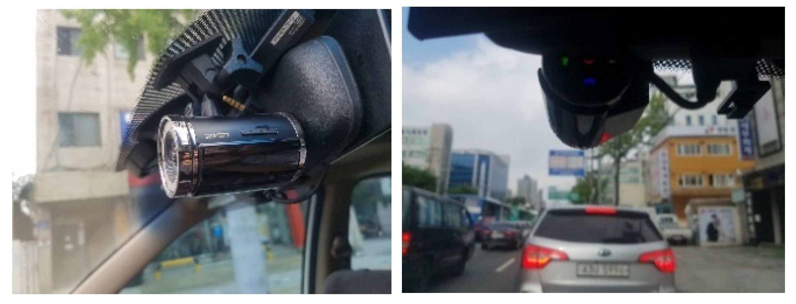
To perform experiments to test the proposed method, images of city roads and highways obtained at various times of the day, and a road image provided by the Karlsruhe vision benchmark [35] were used. To acquire road images, a video-recording device (1920 × 1080, 24-bit MPEG, 15 Hz) attached to the vehicle windscreen was used, as shown in Figure 5. MATLAB was used in a Windows 2010 environment (Dual Hexa Core CPU: 3.3 GHz, RAM: 48 GB), with a Nvidia CUDA GPU (Dual 1080ti) for each parallel-processing stage, using IBM-compatible PCs. For the experiment, the input imaging rate was set to five frames per second, and a 1242 × 375 pixel, 24-bit color RGB image was used as the input image, for VP detection. Processing times for each step in the proposed method have been listed in

Table 4. Experimentally derived average processing times (s).

Steps	Image Analysis	Region of Interest (ROI) Detection	Image Segmentation	Line Detection	VP Selection	Average Time
Time	0.1	0.81	0.26	0.23	0.03	1.43

.

Image-analysis was performed in accordance with the edge information rate of change, instead of using every frame, which shortened average processing times. The ROI-detection process included repeated calculation operations for all pixels, explaining the longer execution time required (see Table 4). Table 4 shows that the average processing time needed for VP detection in the experimental image was approximately 1.43 s implying, that it could be applied in real time. This process was not performed for all input frames although it could be applied in real time using the VP result detected in the previous frame.

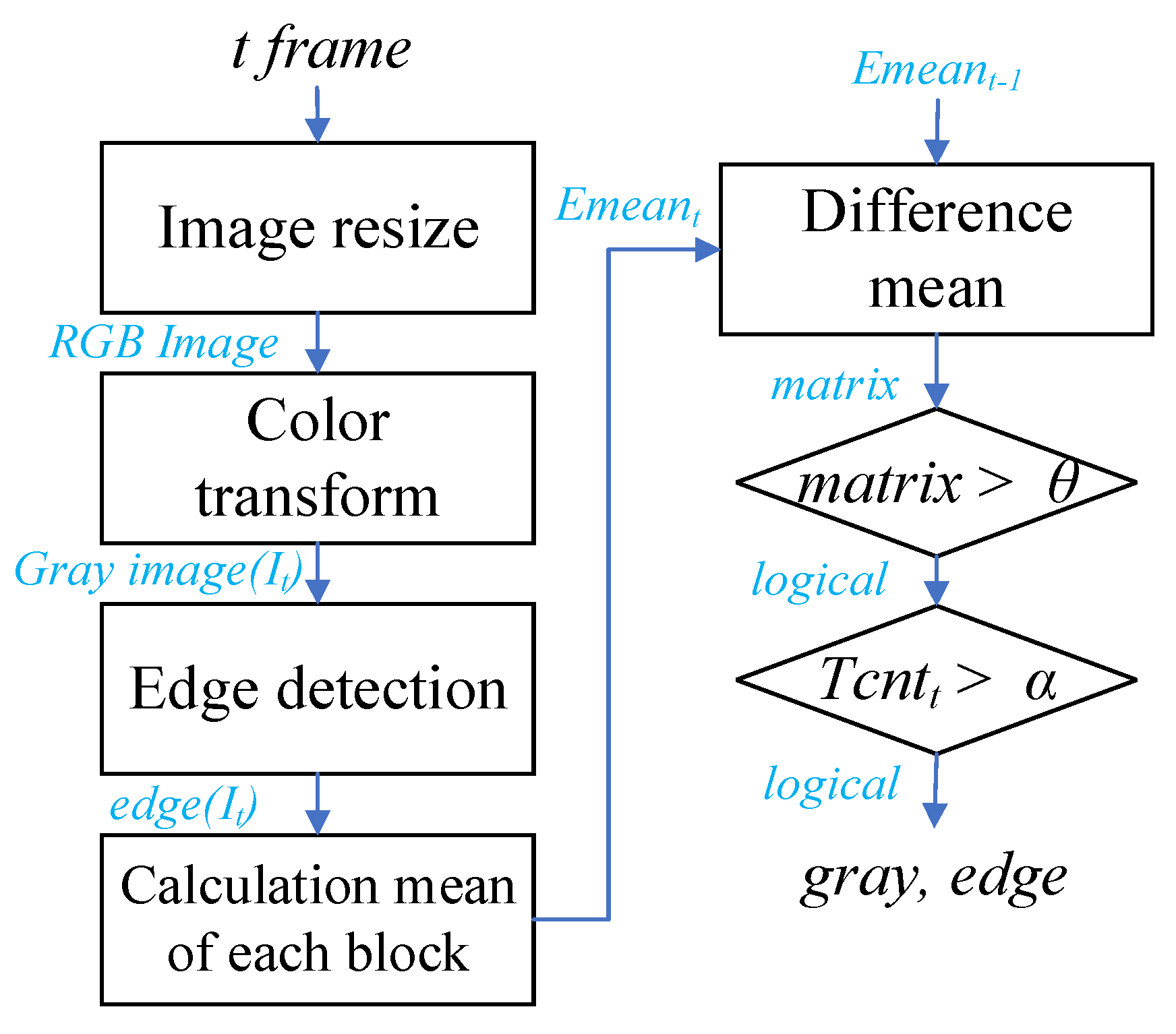
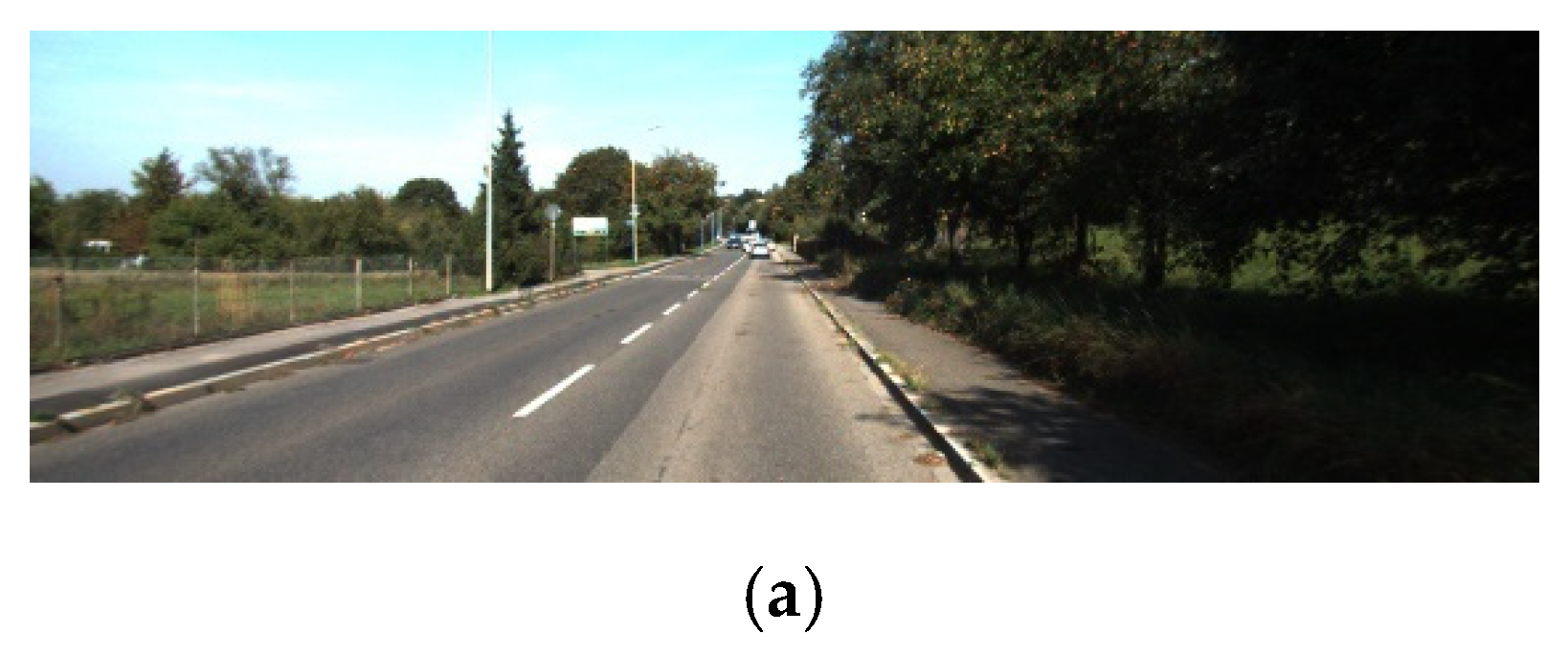
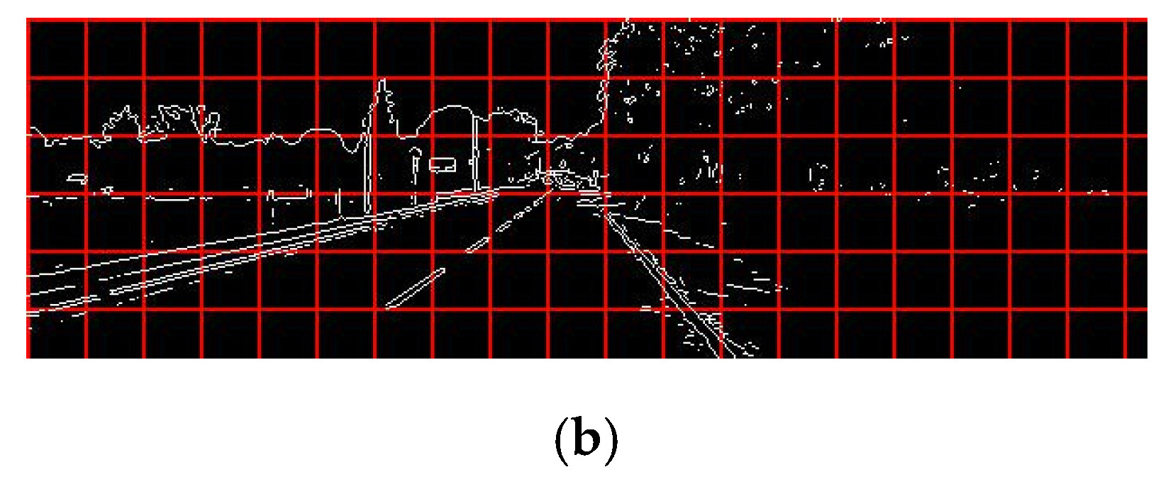
3.1. The Effect of Image Analysis

To perform pre-processing for the image-analysis step, a color image with a pixel size of 1242 × 375 was reduced to half its size, a gray image was transformed, and a 3 × 3 pixel 2D median filter was applied to remove noise. The resultant image (pixel size 621 × 188) was then divided into 70 blocks, each with a pixel size of 32 × 32 pixels, and the Sobel edge pixels were calculated for each block.

After, the number of edge pixels was calculated for each block, the number of blocks in which the number of edge pixels was larger than the threshold value, θ, was then calculated. If this number of blocks was larger than α, the VP detection step was performed for the frame. If the degree of change in the block with the edge pixel number was less than the threshold value α, the position of the VP calculated in the previous frame was also applied to the current frame. The key objective for this step was to avoid the process of calculating VPs for every frame. Therefore, the accuracy of this step had the potential to affect the performance of the entire system, and thus, it was necessary to secure the reliability of these analysis results. Figure 6 shows the changes in the average edge-pixel number differences for the 70 blocks corresponding to each frame of the experimental image.

Figure 6 shows that when many changes occurred in the number of edges between two frames, a large difference in the value existed. In other cases, a value between 0.0 and 0.02 occurred, which meant that no significant change occurred as a feature of the images between adjacent frames. Therefore, threshold value θ, which determined the average number edge-pixel changes in each block corresponding to two adjacent frames, was set to at least 0.02, as shown in Figure 6. Threshold α, which indicates how many of the 70 blocks must be processed when the change occurs, was set to 13, which was the block number where the occurrence probability was greater than 90%, as shown in Figure 6c. Therefore, if the number of blocks with a mean difference value of more than 0.02 blocks between two frames was 13 or more, the VP detection step was performed.

3.2. The Effect of ROI Detection

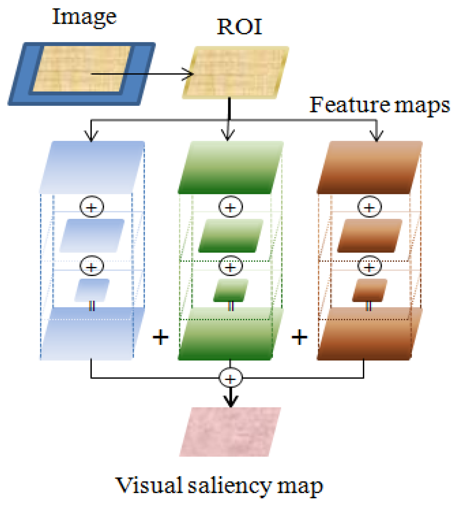
The ROI detection step for a gray image detects the VR using the visual-saliency model. In the VR, visual-saliency values were selected by binarizing just the top 20% of the values, and the ROI was detected and then among the detected VR, the top 20% visual-saliency regions were selected and binarized, to detect the final ROI. A visual-saliency map was created by generating feature maps from the input image, and importance maps were then generated from these feature maps. The feature maps were generated using edge and Gabor filter-based 2D texture orientation (45°, 135°) information from the input image. Therefore, the feature map was represented by three layers using a Gaussian pyramid, and one edge and two components of the directional information were used to form three feature maps. To generate the importance maps, a center-difference operation among the Gaussian parametric levels was then performed, and through this process, the contrast difference between a pixel and its neighbors was calculated, and the visual-saliency pixels were represented by a 2D map. The importance map removed unnecessary regions by increasing the value of the high-value regions in the feature maps and decreasing values for other parts. A visual-saliency map was generated using the sum of the weights (ω₁ = 0.1, ω₂ = 0.2) in Equation (2) for the two importance maps.

Figure 7 shows the results obtained by selecting the top 10% region in the visual-saliency map generated by the visual-saliency model. Figure 7a,b and show the results of the generation of the edge and texture-orientation feature maps from a multiresolution image where the image size was reduced to 50% and 25% of the input image, respectively. The importance map was generated using the feature maps, as shown in Figure 7c, and the visual-saliency map shown in Figure 7d was then generated based on center-difference calculations from the two importance maps. Figure 7e show the result of projecting a visual-saliency map onto the input image, and the visual-saliency map that corresponded to just the top 10% of the value of the visual-saliency map onto the input image, respectively.

3.3. The Effect of Image Segmentation

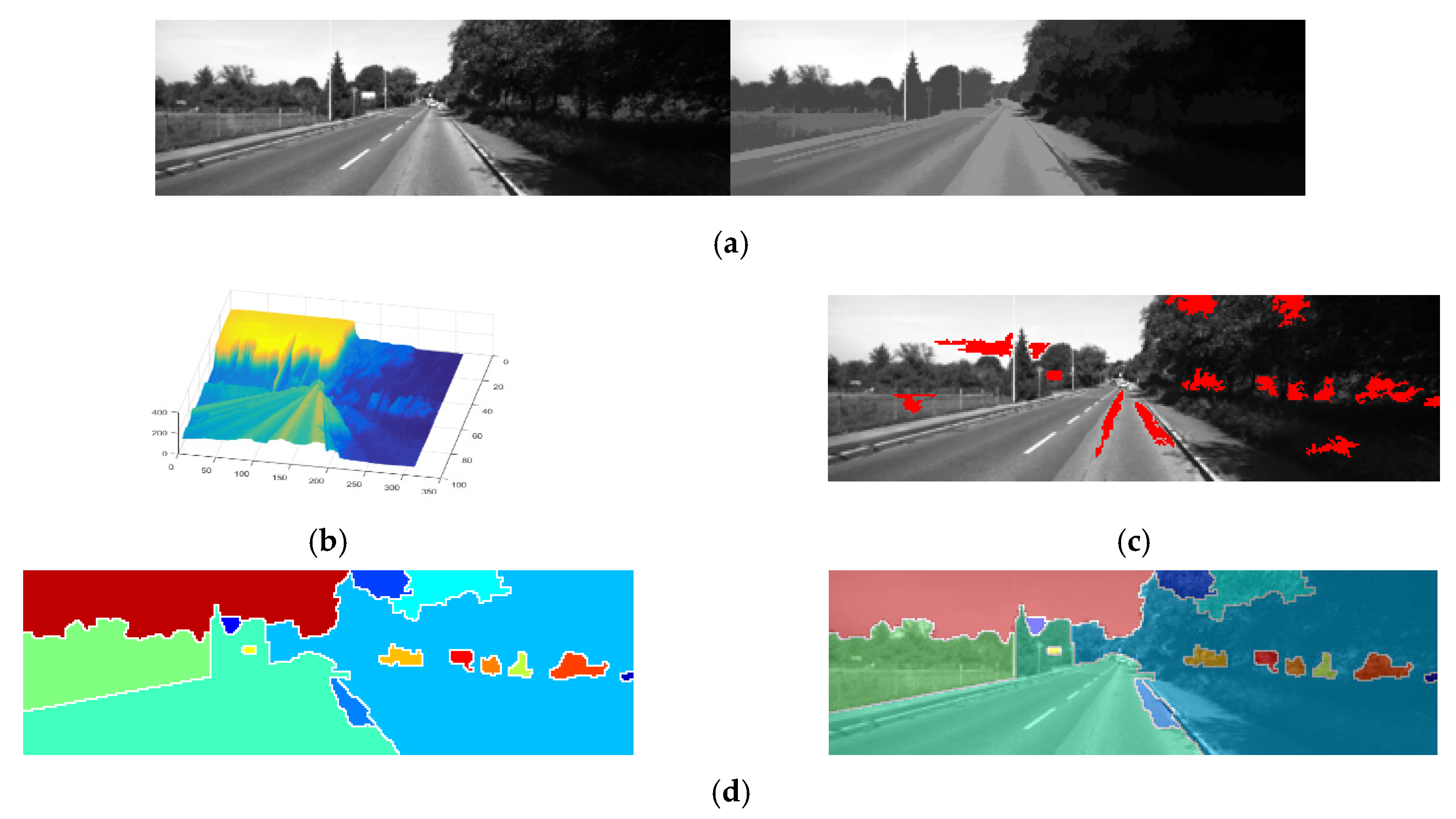
A watershed algorithm based on markers was applied to segment the gray image, although it was not possible to solve the problem in which the image was overdetermined, based only on positioning. To perform this, we needed to distinguish the boundaries of each area clearly, and to solve the problem in which the image was over-segmented in the watershed algorithm, the proposed method designated a marker, which was the initial starting point for image segmentation. Generally, a road image can be divided into a plurality of adjoining regions using connected pixels of similar color and texture, such as the sky and road region where the vehicle is located. In the proposed method, a morphology operation has been applied to the input image, to distinguish the road area from the background area.

To do this, we applied a filtering process using a square operator with a 10 × 10 pixel size. To reduce the execution time and determine the approximate position of the initial marker through the application of multiple morphology operations, computation was performed on image version that was one quarter the size of the input image. In the image segmentation process, the resized input image was combined with the results of the erode- and dilate-reconstruction morphology operations to obtain a smoothed image, as shown in Figure 8a.

We also needed to select an initial marker for watershed image segmentation in the smoothed image. The initial marker selected pixels adjacent to eight directions for each region in the smoothed image and 10 or more pixels connected with a maximum brightness value (Figure 8b,c). Finally, the maximum value of the region was selected as the initial maker, and the image was segmented using the watershed algorithm (Figure 8d). To evaluate image segmentation performance, we compared the image segmentation results obtained using the ground-truth method (Seg_g) with the proposed method (Seg_o) in 70 experimental images. The performance comparison was evaluated in terms of the degree of overlap [(Seg_o∩Seg_g)/Seg_g] between the two segmentation results, and the experimental results demonstrated that the accuracy of the proposed method was greater than 94%.

3.4. The Effect of Line Detection

The Hough transformation was applied to the smoothed gray image in the image segmentation step, to detect straight lines. In the proposed method, we set the maximum Hough peak value to 20, and detected 10 lines that crossed the peak point. In our proposed method, we used line equations to detect the connecting line from the image boundary to the beginning and end, and classified the intersections of these lines as candidate VPs. Figure 9 shows the result of applying the Hough transformation to the input image. The square position in the Hough transformation matrix refers to the peak maximum value.

The theta range was set to [−70:−70, 20:70] to exclude horizontal and vertical lines through the Hough transformation. Following detection of the line intersection points based on the Hough transformation (as shown in Figure 9), only intersections that existed in the candidate region of the actual VP were selected. Intersection selection was performed at the intersection of the lines belonging to the area located from the second to the fourth areas when the image was vertically divided into five parts, and from the second to the third areas, when the image was horizontally divided into five parts, as shown in VP conditions 6 and 7, in Table 1.

3.5. The Effect of VP Selection

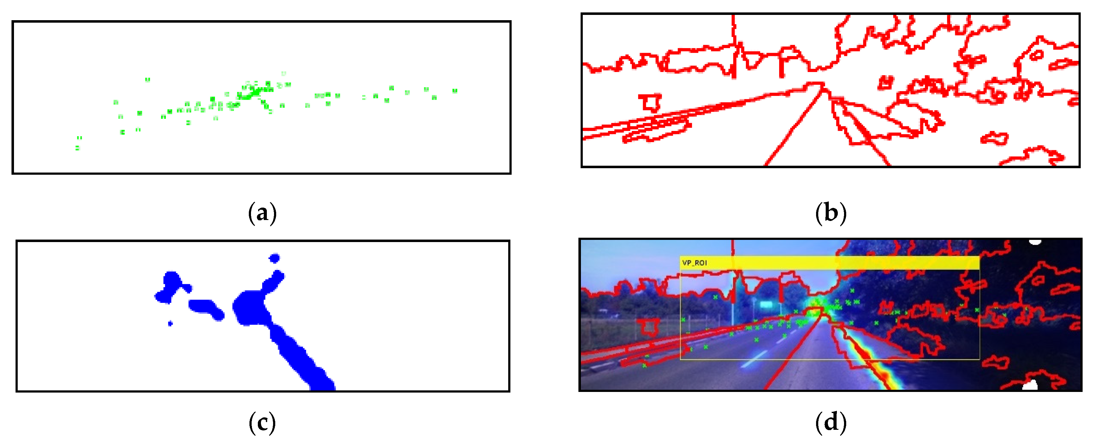
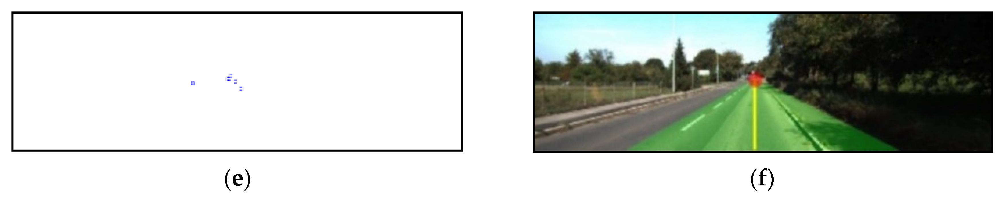
In the proposed method, the VP was selected based on the VRs, the boundaries of the segmented regions (SB), and on line intersection points (CP). For VP selection, the position corresponding to Equation (4) was selected as the VP, while satisfying the VP criteria listed in Table 1. Figure 10 shows VP selection results from the input image initially shown in Figure 3. Figure 10a shows the intersection of the lines detected by the edge based on the Hough transform, and Figure 10b shows the boundaries of the regions segmented by the watershed algorithm. Figure 10c shows the results for the top 10% saliency region detected by the visual-attention model, while Figure 10d shows an overlay of the results of Figure 10a–c in the input image. Figure 10e shows the results obtained by selecting candidate VPs in Figure 10d, and Figure 10f shows the result obtained by selecting the position with the largest value in the VR as the VP, displaying the results on the input image.

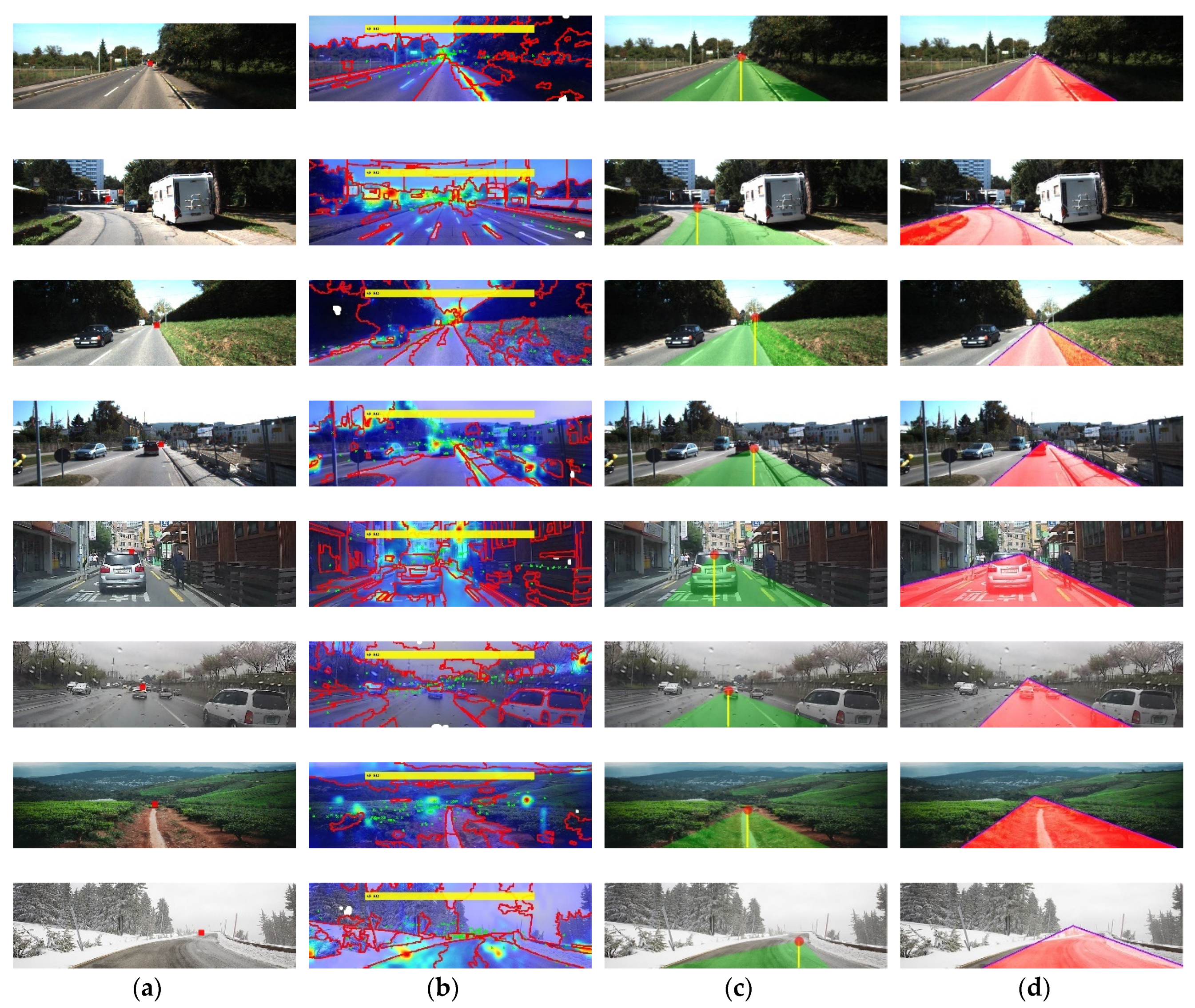
Figure 11 shows results attained for VP detection in various experimental environments. The experiments indicated that detecting the VP using edge information that was not noticeable in a natural image could be challenging, where the influence of roughness, such as a complicated background or a glow, is small. To verify the performance of the proposed method, we compared the ground-truth method, and Li [36] and Kong [37] methods, with the proposed method. The comparison was done using the precision and accuracy obtained using Equation (4), and execution time comparisons were also performed, using the distance differences between the ground-truth method and the VP position coordinates detected using each method.

P = cnt(g_x ∩ a_x)/cnt(a_x)
R = cnt((g_x ∪ a_x) − g_x)/cnt(g_x)

(4)

In Equation (4), a_x refers to the 11 × 11 region where the VP is the center point at x position, detected by the proposed method, and g_x is a binary mask representing the 11 × 11 region detected by the ground-truth method. Here, P is precision, R is recall, and cnt( ) is a counting function.

Consequently, when the VPs were included in the 11 × 11 pixel region, we considered it as a correct detection, and the accuracy was calculated by the error with respect to the VP coordinate set using the ground-truth method.

Table 5. Results of the VP detection in each road environment.

	Measures	Precision(P)	Recall(R)	Processing Time (s)
Methods
Highway (vehicle only)
Li’s method [36]		85	81	0.63
Kong’s method [37]		97	96	4.10
Proposed method		93	92	1.41
City roads
Li’s method [36]		82	84	0.67
Kong’s method [37]		94	97	4.40
Proposed method		95	93	1.43
Other roads
Method in [36]		87	83	0.65
Kong’s method [37]		93	96	4.20
Proposed method		91	90	1.47

presents comparison results, in terms of precision, recall, and processing time for VP detection, in the experimental images.

Figure 11 shows VP location based on the ground-truth method, with Figure 11a–d showing VP selection results obtained using the ground-truth method, our method, and Kong’s method [36]. These results showed that, when comparing total execution time, Kong’s method needed an execution time three times longer than the proposed method based on VP detection using a voting system for all pixels.

4. Conclusions

In this paper, we have proposed an efficient VP detection method that can be applied to autonomous vehicles, in an effort to support safe driving. By detecting the VP, various ADASs such as prediction of the traveling direction of a vehicle, detection of an omnidirectional object, and prevention of lane departure on the road can be employed. To detect the VP in a vehicle driving situation, accurate and real-time processing must be performed, and we have proposed a simple and fast detection method that processes images in advance and in real time without processing all frames. The proposed method achieved outcomes through selective detection of the VP, and has been based on a specific VP definition. Comparison of the proposed method with the ground-truth method showed that the former demonstrated good performance, however, as our method is fundamentally influenced by illumination, coping with environmental influences, such as nighttime, or fog, has proved difficult. Future research will explore a VP detection system that can overcome these environmental limitations using either infrared or thermal-imaging equipment.

References

1. Kuutti, S.; Fallah, S.; Katsaros, K.; Dianati, M.; Dianati, M.; Mccullough, F.; Mouzakitis, A. A Survey of the State-of-the-Art Localization Techniques and Their Potentials for Autonomous Vehicle Applications. IEEE Internet Things J. 2018, 5, 829–846. [Google Scholar]
2. Morales, N.; Toledo, J.; Acosta, L.; Medina, J.S. A Combined Voxel and Particle Filter-Based Approach for Fast Obstacle Detection and Tracking in Automotive Applications. IEEE Trans. Intell. Transp. Syst. 2017, 18, 1824–1834. [Google Scholar] [CrossRef]
3. Kwon, Y.H. Improving Multi-Channel Wave-Based V2X Communication to Support Advanced Driver Assistance System (ADAS). Int. J. Automot. Technol. 2016, 17, 1113–1120. [Google Scholar] [CrossRef]
4. Choi, H.C.; Kim, S.Y.; Oh, S.Y. In and out vision-based driver-interactive assistance system. Int. J. Automot. Technol. 2010, 11, 883–892. [Google Scholar] [CrossRef]
5. Woo, J.W.; Yu, S.B.; Lee, S.B. Design and simulation of a vehicle test bed based on intelligent transport systems. Int. J. Automot. Technol. 2016, 17, 353–359. [Google Scholar] [CrossRef]
6. Nieto, M.; Velez, G.; Otaegui, O.; Gaines, S.; Cutsem, G.V. Optimising computer vision based ADAS: Vehicle detection case study. IET Intell. Transp. Syst. 2016, 10, 157–164. [Google Scholar] [CrossRef]
7. Lee, H.J.; Moon, B.; Kim, G. Hierarchical Scheme of Vehicle Detection and Tracking in Nighttime Urban Environment. Int. J. Automot. Technol. 2018, 19, 369–377. [Google Scholar] [CrossRef]
8. Dopico, J.G.; Pedraza, J.L.; Nieto, M.; Perez, A.; Rodriguez, S.; Osendi, L. Locating moving objects in car-driving sequences. Eurasip J. Image Video Process. 2014, 24, 1–23. [Google Scholar]
9. Kim, J.B. Automatic vehicle license plate extraction using region-based convolutional neural networks and morphological operations. Symmetry 2019, 11, 882. [Google Scholar] [CrossRef] [Green Version]
10. Kang, C.; Heo, S.W. Intelligent safety information gathering system using a smart black box. In Proceedings of the 2017 IEEE International Conference on Consumer Electronics (ICCE), Las Vegas, NV, USA, 8–10 January 2017; pp. 229–230. [Google Scholar]
11. Kim, J.W.; Kim, S.K.; Lee, S.H.; Lee, T.M.; Lim, J.H. Lane recognition algorithm using lane shape and color features for vehicle black box. In Proceedings of the 2018 International Conference on Electronics, Information, and Communication (ICEIC), Honolulu, HI, USA, 24–27 January 2018; pp. 1–2. [Google Scholar]
12. Mohamedaslam, C.; Ajmal, R.T.; Mohamed, S.M.T.; Najeeb, N.A.; Nisi, K. A smart vehicle for accident prevention using wireless blackbox and eyeblink sensing technology along with seat belt controlled ignition system. In Proceedings of the 2016 Online International Conference on Green Engineering and Technologies (IC-GET), Coimbatore, India, 19 November 2016; pp. 1–6. [Google Scholar]
13. John, N.; Anusha, B.; Kutty, K. A reliable method for detecting road regions from a single image based on color distribution and vanishing point location. Procedia Comput. Sci. 2015, 58, 2–9. [Google Scholar] [CrossRef] [Green Version]
14. Li, Y.; Ding, W.; Zhang, X.G.; Ju, Z. Road detection algorithm for autonomous navigation systems based on dark channel prior and vanishing point in complex road scenes. Robot. Auton. Syst. 2016, 85, 1–11. [Google Scholar] [CrossRef] [Green Version]
15. Gallagher, A.C. A ground truth based vanishing point detection algorithm. Pattern Recognit. 2002, 35, 1527–1543. [Google Scholar] [CrossRef]
16. Rother, C. A new approach to vanishing point detection in architectural environments. Image Vis. Comput. 2002, 2, 647–655. [Google Scholar]
17. Tsai, T.H.; Fan, C.S. Monocular vision-based depth map extraction method for 2D to 3D video conversion. Eurasip J. Image Video Process. 2016, 21, 1–12. [Google Scholar] [CrossRef] [Green Version]
18. Shi, J.; Wang, J.; Fu, F. Fast and robust vanishing point detection for unstructured road following. IEEE Trans. Intell. Transp. Syst. 2016, 17, 970–979. [Google Scholar] [CrossRef]
19. Zhang, Y.; Su, Y.; Yang, J.; Ponce, J.; Kong, H. When Dijkstra meets vanishing point: A stereo vision approach for road detection. IEEE Trans. Image Process. 2018, 27, 2176–2188. [Google Scholar] [CrossRef]
20. Yang, W.; Fang, B.; Tang, Y.Y. Fast and accurate vanishing point detection and Its application in inverse perspective mapping of structured road. IEEE Trans. Syst. Man Cybern. Syst. 2018, 48, 755–766. [Google Scholar] [CrossRef]
21. Ebarhimpour, R.; Rasoolinezhad, R.; Haiiabolhasani, Z.; Ebrahimi, M. Vanishing point detection in corridors: Using Hough transform and K-means clustering. IET Comput. Vis. 2012, 6, 40–51. [Google Scholar] [CrossRef]
22. Lutton, E.; Maitre, H.; Krahe, J.L. Contribution to the determination of vanishing points using Hough transform. IEEE Trans. Pattern Anal. Mach. Intell. 1994, 16, 430–438. [Google Scholar] [CrossRef]
23. Kim, J.B. Hough transform-based road detection for advanced driver assistance systems. In International Conference on Intelligent Science and Big Data Engineering; Lecture Notes in Computer Science (LNCS); Springer: Cham, Switzerland, 2015; Volume 9242, pp. 281–287. [Google Scholar]
24. Barnard, S.T. Interpreting perspective images. Artif. Intell. 1983, 21, 435–462. [Google Scholar] [CrossRef]
25. Kong, H.; Sarma, S.E.; Tang, F. Generalizing laplacian of gaussian filters for vanishing-point detection. IEEE Trans. Intell. Transp. Syst. 2013, 14, 408–418. [Google Scholar] [CrossRef]
26. Suttorp, T.; Bucher, T. Robust Vanishing point estimation for driver assistance. In Proceedings of the 2006 IEEE Intelligent Transportation Systems Conference, Toronto, ON, Canada, 17–20 September 2006; pp. 17–20. [Google Scholar]
27. Choi, H.C.; Kim, C. Real-time vanishing point detection using histogram of oriented gradient. J. Inst. Electron. Inf. Eng. 2011, 48, 96–101. [Google Scholar]
28. Kim, J.B. Efficient vanishing point detection for advanced driver assistance system. Adv. Sci. Lett. 2017, 23, 4114–4118. [Google Scholar] [CrossRef]
29. Hoiem, D.; Efros, A.A.; Hebert, M. Putting objects in perspective. Int. J. Comput. Vis. 2008, 80, 3–15. [Google Scholar] [CrossRef]
30. Gonzalez, R.C.; Woods, R.E. Digital Image Processing, 3rd ed.; Prentice Hall: Upper Saddle River, NJ, USA, 2007. [Google Scholar]
31. Kim, J.B. Efficient detection of direction indicators on road surfaces in car black-box for supporting safe driving. Int. J. Internet Broadcast. Commun. 2015, 7, 123–129. [Google Scholar]
32. Kim, J.B. Detection of traffic signs based on eigen-color model and saliency model in driver assistance systems. Int. J. Automot. Technol. 2013, 14, 429–439. [Google Scholar] [CrossRef]
33. Tian, H.; Fang, Y.; Zhao, Y.; Lin, W.; Ni, R.; Zhu, Z. Salient region detection by fusing bottom-up and top-down features extracted from a single image. IEEE Trans. Image Process. 2014, 17, 4389–4398. [Google Scholar] [CrossRef]
34. Itti, L.; Koch, C.; Niebur, E. A model of saliency-based visual attention for rapid scene analysis. IEEE Trans. Pattern Anal. Mach. Intell. 1998, 20, 1254–1259. [Google Scholar] [CrossRef] [Green Version]
35. The KITTI Vision Benchmark Suite. Karlsruhe Institute of Technology. Available online: http://ww.cvlibs.net/datasets/kitti/eval_road.php (accessed on 1 June 2019).
36. Li, B.; Peng, K.; Ying, X.; Zha, H. Simultaneous vanishing point detection and camera calibration from single images. In International Symposium on Visual Computing; Lecture Notes in Computer Science (LNCS); Springer: Berlin/Heidelberg, Germany, 2010; Volume 6454, pp. 151–160. [Google Scholar]
37. Kong, H.; Audibert, J.Y.; Ponce, J. Vanishing point detection for road detection. In Proceedings of the 2009 IEEE Conference on Computer Vision and Pattern Recognition, Miami, FL, USA, 20–25 June 2009; pp. 96–103. [Google Scholar]
Figure 1. Flowchart of the proposed method. (a) Processing flow, (b) image matrix transformation flow.
Symmetry 11 01492 g001
Figure 2. Flowchart of the image-analysis step.
Symmetry 11 01492 g002
Figure 3. Input image and edge with block result. (a) Input road image, (b) edge image of (a) with 32 × 32 blocks.
Symmetry 11 01492 g003aSymmetry 11 01492 g003b
Figure 4. Flowchart for visual-attention region detection.
Symmetry 11 01492 g004
Figure 5. Experimental setup for image acquisition.
Symmetry 11 01492 g005
Figure 6. Results from detecting threshold values in the image-analysis step: average block difference and number of blocks above θ = 0.02. (a) Differences in the average edge pixel numbers per block between adjacent frames, (b) differences in the value of the average block edge change (left: frame without scene change; right: frame with scene change), (c) probability of a block exceeding the threshold (θ = 0.02).
Symmetry 11 01492 g006
Figure 7. Results and processes of the detection of the visual-saliency map. (a) Edge feature map, (b) texture orientation feature map [45° (left), 135° (right)], (c) importance map, (d) visual-saliency 3D and 2D maps, (e) input image with visual-saliency map, (f) image with top 10% visual-saliency map.
Symmetry 11 01492 g007
Figure 8. Results obtained for image over-segmentation using the watershed algorithm. (a) Gray image and result from the morphology operation, (b) three-dimensional (3D) result from the morphology operation, (c) result after marker selection, (d) results after image segmentation.
Symmetry 11 01492 g008
Figure 9. Results of the line detection using the Hough transform. (a) Smoothed image, (b) edge image of (a), (c) results of the Hough transformation and the Hough peak value, (d) result of the line detection (⋆ denotes the cross point of the lines).
Symmetry 11 01492 g009
Figure 10. Results from VP selection on Figure 3. (a) Intersection of the straight lines, (b) boundaries of the regions segmented, (c) saliency region, (d) overlay result of (ac), (e) candidate VPs; (f) VP detection result.
Symmetry 11 01492 g010aSymmetry 11 01492 g010b
Figure 11. Results of the VP detection. (a) Ground truth method, (b) processing results, (c) proposed method, (d) method in [29].
Symmetry 11 01492 g011