A Multifactor Fuzzy Time-Series Fitting Model for Forecasting the Stock Index

Abstract

Fuzzy time series (FTS) models have gotten much scholarly attention for handling sequential data with incomplete and ambiguous patterns. Many conventional time series methods employ a single variable in forecasting without considering other variables that can impact stock volatility. Hence, this paper modified the multi-period adaptive expectation model to propose a novel multifactor FTS fitting model for forecasting the stock index. Furthermore, after a literature review, we selected three important factors (stock index, trading volume, and the daily difference of two stock market indexes) to build a multifactor FTS fitting model. To evaluate the performance of the proposed model, the three datasets were collected from the Nasdaq Stock Market (NASDAQ), Taiwan Stock Exchange Index (TAIEX), and Hang Seng Index (HSI), and the RMSE (root mean square error) was employed to evaluate the performance of the proposed model. The results show that the proposed model is better than the listing models, and these research findings could provide suggestions to the investors as references.

1. Introduction

Humans have attempted to forecast future events based on past history since ancient times. Consequently, people have constantly endeavored to develop new technologies for making better predictions. In recent decades, numerous scholars have proposed many fuzzy time series (FTS) methods for improving the forecast performance. Song and Chissom [1] first presented a FTS model, and many different FTS models have been subsequently proposed for forecast in various domains, such as university enrollment [2,3,4,5], stock indexes [6,7,8,9,10] and meteorology [11,12]. For investors, forecasting the stock index is a very important topic; many profits can be earned if we can accurately predict stock trends accurately. Many factors can affect the stock market and cause market volatility, such as global economic conditions, domestic macroeconomic factors, and highly relevant foreign stock markets. However, most of the time series models employ the stock index as the only factor in forecasting and ignore other important factors [13]. Intuitively, a better result for the forecast can be obtained if we consider more variables when making predictions [14].

Since the 1990s, we have experienced many financial crises, such as the 1994 Mexican financial crisis, the 1997 Asian financial crisis, and the 2008 global financial tsunami. As a result, international financial markets have undergone numerous changes, the most critical being that large amounts of money are now free to flow between without restrictions between any governments. In the context of this liberalization and globalization of international capital flow, the stock market reflects all economic activities worldwide. Consequently, using the stock price index, we can gauge the economic circumstances of a country. Finding a pattern in the fluctuations of a country’s stock market would benefit forecasting the future trends of a country’s economy. It would also provide information for enterprises and investors to help them make decisions. Dickinson [15] showed that international stock markets can lead to the fluctuations in global stock indexes. For individual investors, stocks are highly profitable financial products but involve high risk. The stock market is a dynamic environment, and obtaining precise information is crucial for planning investments of investors.

Trading volume is a fundamental factor suitable for use in long-term forecasting [16]. Many researchers have reported a relationship between stock index and trading volume [6,17,18,19,20,21,22,23,24]. Campbell et al. [18] showed the relationship between the trading volume of the stock market and the daily serial stock returns. Hiemstra and Jones [20] presented the evidence of a clear two-direction nonlinear causal relationship between returns and trading volumes. Rashid [17] showed that volume has an important non-linear explanatory power for stock returns. However, stock returns have a linear relation with trading volumes, which indicates that one of these factors can improve forecast by knowledge of the other. Zhu et al. [22] demonstrated that volume can enhance the medium-term and long-term forecasts in neural networks. Le and Zurbruegg [23] proposed using trading volume to improve the forecasts in various autoregressive conditional heteroscedasticity (ARCH) models.

In the soft computing techniques, artificial neural networks (ANNs) are used in most cases due to their performance in nonlinear systems. To deal with the problem of nonlinear or nonstationary time series, many notable studies on adaptive neuro-fuzzy models (ANFISs) have been done by Su and Cheng [25], Stefanakos [26], and others. Therefore, the motivation for this study is based on three factors used to fit a linear combination of multifactor fuzzy time-series to forecast the stock index, because a linear model is simple and easily explained. As mentioned above, this study proposed a novel multifactor FTS model based on stock volatility to forecast a stock index. The trading volume, stock index, and interaction between two stock markets were employed as forecasting factors in the proposed model, and the optimal parameters α, β, and γ are obtained through training.

The remaining section is organized as follows: The related work is presented in Section 2; Section 3 outlines the proposed model; Section 4 shows the verification and comparison; Section 5 presents the findings; and Section 6 is the conclusions.

2. Related Work

This section briefly reviews the FTS and causality relationship between price and volume.

2.1. Fuzzy Time Series

Fuzzy theory [27] was first employed to solve the linguistic values problems. Song and Chissom [1,25] applied fuzzy theory to a time series model to forecast student enrollment. Soon, Song and Chissom [28] also defined a one-order time invariant FTS model to forecast enrollment. Later, Chen [4] presented a FTS model that produced a more accurate forecast than that of [1] by applying simplified arithmetical operations in forecasting algorithms. Bose and Mali [29] summarized and reviewed the past 25 years of Elsevier journals on fuzzy time series forecasting during 1993–2018, they were based on FTS forecasting models with five main steps (define range, partition range into intervals, fuzzifiy the dataset, build a fuzzy logical relationship (FLR) and FLR group (FLRG), and defuzzify the fuzzy value) to classify into two main contribution phases: (1) the data partitioning Phase and (2) the prediction phase.

For partitioning, Chen et al. [30] proposed a new FTS forecasting method based on the proportions of intervals and particle swarm optimization (PSO) techniques; they used PSO techniques to obtain the optimal partitions of intervals. In forecasting, an important factor impacting the forecasting performance of fuzzy TSF models is FLRs. Traditionally, the rule-based methods have been used to build FLRs [29]. However, to reduce the computational complexity and improve the forecast accuracy, authors have used ANNs [31,32], fuzzy inference systems [33], support vector regression [34], and a general regression neural networks [35] as alternatives. For a multi-factors FTS, Chen and Chen [36] proposed a leverage of fuzzy variations between the main factor and the secondary factor to forecast the TAIEX. Huarng et al. [37] also presented a multivariate heuristic model for fuzzy time-series forecasting.

The current FTS approach benefits both theoretical development and related applications, which offers wider uses. This trend indicates that the development of FTS has improved significantly. Especially, artificial intelligence is used in most forecast problems due to its performance for nonlinear systems. In nonlinear or nonstationary time series, many studies on adaptive neuro-fuzzy models (ANFIS) have been proposed, such as those by Su and Cheng [25] and Stefanakos [26].

2.2. The Causality between Price and Volume

In financial prediction, we usually use the price as an index to predict the financial trend. In the stock market, price fluctuations will impact the investor’s mind and behavior. Volume is a measure of market liquidity, while index refers to the price. If there is a relationship between the volumes and fluctuations of price, the trading volume is higher than the average level, which generally represents the real trend of the price.

Recently, Tsai [38] used the average price and transaction volume of existing houses to analyze the dynamic price–volume causality in the American housing market; he applied a rolling window sample to estimate the relationship in the bootstrap Granger causality test, and the results reveal that the transaction volume tends to be informative during price rigidity. Previously, most investors have paid attention to the relationship between volume and stock returns, but recent studies have begun to show a dynamic relationship (causality) between the daily share returns and trading volumes, following the concept of Granger causality [39]. The circumstance above could be found in the multinational stock market and used to enhance the accuracy of predicting the stock price and forecasting the trend of the stock market index [40,41,42,43]. To correctly forecast stock price, experts have studied the technical analysis indicators and proven the significance of these indicators. The volume ratio value is verified to be a significant technical indicator and is used in our proposed model [44].

However, to obtain the better forecasting, more factors must to be added in the FTS model, and the causal relationship of the FTS should be considered. The high-order time-series models must also be employed. Lee et al. [14] has proposed a two-factor and high-order FTS, which has been proven to be highly efficient.

3. Proposed Model

Stock market volatility is affected by many variables, such as global economic conditions, the domestic macroeconomy, and highly interrelated foreign stock markets. In previous studies, many time series models only employed the stock index as a single factor in forecasting and ignored other factors. To improve accuracy, more factors should be considered in stock forecasting models.

Previous studies paid attention to the relationship between stock returns and trading volume, but many researchers have begun to present the dynamic relationship between daily trading volume and stock returns, which is named “causality” [20]. Stock market causalities have shown a correlation between trading volume and the stock market index. Hence, the trading volume must be added as a factor in stock index forecasting.

Likewise, both academics and investors have given considerable attention to the interactions between different stock markets when forecasting a stock index. The practical experience of stock market investors has shown that the relationships between different stock markets are enough to be noticeable; therefore, numerous investors have utilized the fluctuations of other stock markets that significantly affect their respective domestic markets as the basis for forecasting [13]. Lee et al. [45] looked for spillovers from the returns of the Nasdaq Stock Market (NASDAQ) and volatility in Asian second board markets after checking for spillovers from the New York Stock Exchange and discovered strong evidence of staggered spillovers from the NASDAQ to Asian markets when concurrent main board market returns were excluded. Yang [46] proved that the price change spillover effects from the NASDAQ were significant for both the Taiwan Stock Exchange Index (TAIEX) and the Taiwan Electronic Sector Index Futures (TEXF), with close-to-close returns being the most strongly affected. Because of the time difference between the United States and Taiwan, the opening price of the Taiwan stock market might show an overreaction in its close-to-open rate of return. Following the overreaction of the opening price, the market index would adjust to the proper price during trading hours. Other studies have clearly described the significant interaction between two stock markets [47,48]. Therefore, in this study, the NASDAQ, TAIEX, and Hang Seng Index (HSI) were used as experimental datasets with which to forecast a stock index in this study.

Most stock markets forecasting models developed have three major drawbacks: (1) they employ the stock index as the only single factor in forecasting; (2) they include only the causality between the trading volume and stock index; and (3) they consider the interactions between only two stock markets. To overcome these drawbacks, this paper refers to [49] to improve the proposed method and experiment. The proposed model extends the multi-period adaptation model in [7] by including the three crucial factors mentioned: stock index, trading volume of stock, and the interactions between two stock markets. The procedure of the proposed model is shown in Figure 1.

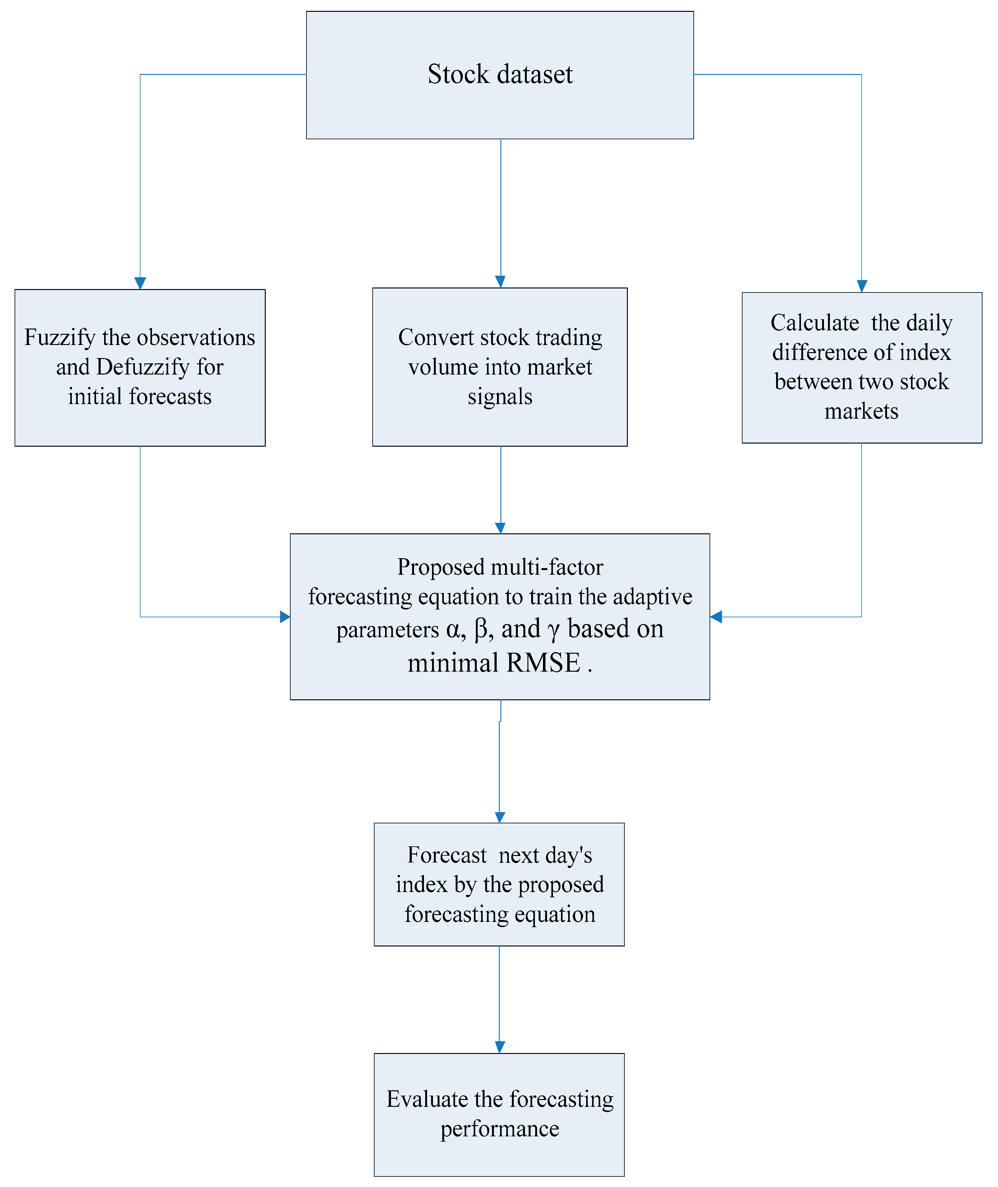
3.1. Proposed Computational Step

As mentioned above, this paper proposes a multi-factor fuzzy time series model to improve performance for stock forecasting. The proposed computational methods entails eight steps: (1) Collect datasets; (2) fuzzify the observations and defuzzify F(t) to obtain the initial forecast; (3) transfer trading volume into market signals; (4) calculate the daily difference of the indexes between two stock markets; (5) propose a multi-factor forecasting Equation; (6) adapt the best parameters for α, β and γ; (7) forecast the stock index; and (8) evaluate the forecasting performance. To detail the proposed model, each step of the proposed algorithm is described as follows:

Step 1. Collect the datasets.

The experimental datasets include three financial datasets (1) The TAIEX dataset, comprising the stock index from 03/01/1997 to 31/12/2004, was collected from the Taiwan Economic Journal (TEJ), (2) The HSI dataset, comprising the stock index from 1997/01/02 to 2004/12/31, was also collected from the TEJ database, and (3) The NASDAQ dataset, comprising the stock index from 1997/01/02 to 2004/12/31, was collected from the Yahoo website database (http://finance.yahoo.com/).

Step 2. Fuzzify the data and defuzzify F(t) to obtain an initial forecast.

(1) Determine the range and linguistic values.

Determine the range X = [min, max], which covers all observed stock index (training dataset). For example, the min and max values of TAIEX from 1997/01/03 to 2004/12/31 are 3446 and 10,202, respectively. The range is thus defined as X = [3446, 10,202]. Miller [50] suggested that the appropriate number of categories is seven (or 7 ± 2) because of the limitations of short-term human memory. Hence, the range is divided initially into seven equal linguistic intervals. Then the average datum for each linguistic value can be calculated. The length of the linguistic interval in this study is (10,202 − 3446)/7 = 965; thus, there are seven linguistic intervals: [3446, 4411], [4411, 5377], [5377, 6342], [6342, 7307], [7307, 8272], [8272, 9237], and [9237, 10,202].

(2) Build fuzzy sets and fuzzify the historical data.

Build the fuzzy set B₁, B₂, … B_k in the following range:

$$\begin{array}{c}{B}_1=\frac{b_{11}}{u_1}+\frac{b_{12}}{u_2}+\dots +\frac{b_{1m}}{u_m}\\ B_2=\frac{b_{21}}{u_1}+\frac{b_{22}}{u_2}+\dots +\frac{b_{2m}}{u_m}\\ \begin{array}{c}⋮\\ B_k=\frac{b_{k1}}{u_1}+\frac{b_{k2}}{u_2}+\dots +\frac{b_{km}}{u_m}\end{array}\end{array}$$

(1)

where b_ij is the grade of u_j in fuzzy set B_i, 1 ≤ i ≤ k, 1 ≤ j ≤ m, and b_ij ∈ [0,1].

Determine the grade of each historical datum belonging to each B_i (i = 1… m). If the maximal grade is located in B_k, then we mark the fuzzified stock index as B_k. The following seven linguistic values were used in this study: B₁ (very low), B₂ (low), B₃ (slightly low), B₄ (normal), B₅ (slightly high), B₆ (high), and B₇ (very high).

(3) Build fuzzy logical relationships (FLRs)

From the two consecutive fuzzy sets, B_i (t − 1) and B_j (t), we can use B_i→B_j to represent fuzzy logical relationships. i.e., “If part (rule condition)” is the value of the t trading day, and “Then part (rule conclusion)” is the value of the t + 1 trading day. The five TAIEX stock trading days from 2000/03/17 to 2000/3/23 are used as an example in the FLR in

Table 1. FLR table for time series.

TAIEX’s Rule for Consecutive Trading Day	FLR
8763.27 (t = 2000/03/17)→8536.05 (t + 1 = 2000/03/20)	B6 (t)→B5 (t + 1)
8536.05 (t = 2000/03/20)→9004.48 (t + 1 = 2000/03/21)	B5 (t)→B6 (t + 1)
9004.48 (t = 2000/03/21)→9069.39 (t + 1 = 2000/03/22)	B6 (t)→B6 (t + 1)
9069.39 (t = 2000/03/22)→9533.87 (t + 1 = 2000/03/23)	B6 (t)→B7 (t + 1)

t denotes trading day.

. For example, in the second row of Table 1, the trading day 8763.27 (t = 2000/03/17) falls into B₆ and the next trading day 8536.05 (t + 1 = 2000/03/20) falls into B₅ (please refer seven linguistic intervals in step II (1)); then, the FLR can be represented as B₆ (t)→B₅ (t + 1).

(4) Merge all FLRs

We use the same left-hand sides to merge FLRs and form a FLRs group. For instance, B_i→B_j, B_i→B_k, B_i→B_m can be grouped as B_i→B_j, B_k, B_m. A fluctuation-type stock index has three trends: upward trend, no change, and downward trend; these three trends are used to express the FLRs group. The range of the stock index is partitioned into seven linguistic terms in this paper. As mentioned, price fluctuation is used to group the FLRs. For example, B₁→B₂ is grouped as an “upward” trend, B₁→B₁ is “no change”, and B₂→B₁ is a “downward” trend.

(5) Give weights to all FLRs groups

Using the fluctuation-weighted approach [51], we assign weights to all FLR groups, and normalize all weights to a normalized weight matrix, W_n(t), as presented in Equation (2):

$$W_n\left(t\right)=\left[\begin{array}{ccc}{w}_1,& w_2,& \begin{array}{cc}\dots & w_n\end{array}\end{array}\right]=\left[\begin{array}{ccc}\frac{W_1}{{{\displaystyle \sum }}_{k=1}^n{W}_k},& \frac{W_2}{{{\displaystyle \sum }}_{k=1}^n{W}_k},& \begin{array}{cc}\dots & \frac{W_n}{{{\displaystyle \sum }}_{k=1}^n{W}_k}\end{array}\end{array}\right]$$

(2)

(6) Defuzzify F(t + 1) to obtain the initial forecast.

The defuzzified forecast F(t + 1)_df and the defuzzified matrix L_df(t), which are defined as Equations (3) and (4), respectively, are applied in this step. The defuzzified value then denotes the initial stock index forecast.

$$\mathrm{F}{\left(\mathrm{t}+1\right)}_{\mathrm{df}}=L_{df}\left(t\right)W_n\left(t\right)$$

(3)

$$L_{df}\left(t\right)=\left[\begin{array}{ccc}{m}_1& m_2& \begin{array}{cc}\dots & m_i\end{array}\end{array}\right]$$

(4)

where m_i is the intermediate point of each linguistic interval, L_i.

Step 3. Transfer the trading volume into market signals.

(1) The daily trading volume is converted into a technical indicator of volume VR(t) as follows:

$$VR(t)=\frac{{\displaystyle \sum _{i=1}^n{V}_{up}(t)-{\displaystyle \sum _{i=1}^n{V}_{down}(t)}}}{{\displaystyle \sum _{i=1}^{n}V(t)}}$$

(5)

where ${\displaystyle \sum }_{j=1}^n{V}_{up}\left(t\right)$ is the sum of trading volumes, if the stock market closes on an upward trend for the previous n days; and ${\displaystyle \sum }_{j=1}^n{V}_{down}\left(t\right)$ is the sum of the trading volumes, if the stock market closes on downward trend for the previous n days

(2) Define the range of VR(t).

The range X = [low, high], which covers all observations VR(t) in the training dataset. This range is initially partitioned into five linguistic intervals L_i based on stock market properties.

(3) Build fuzzy sets of VR(t) and fuzzify the VR(t) observations.

Define fuzzy set L₁, L₂, … L_k in the range by using Equation (1). Then fuzzify all data into five linguistic values, defined as follows: L₁ (oversold), L₂ (sold), L₃ (stable), L₄ (bought), and L₅ (overbought).

(4) Convert linguistic terms into market signals.

The function of the signal transfer is defined in Equation (6). This function can be used to transfer all possible linguistic terms into the corresponding market signals.

$$M\left(L_{VR\left(t\right)}\right)=\{\begin{array}{c}\begin{array}{cc}+1,& if L_{VR\left(t\right)} is L_1\end{array}\\ \begin{array}{cc}+0.5,& if L_{VR\left(t\right)} is L_2\end{array}\\ 0\begin{array}{cc},& if L_{VR\left(t\right)} is L_3\end{array}\\ \begin{array}{cc}-0.5,& if L_{VR\left(t\right)} is L_4\end{array}\\ \begin{array}{cc}-1,& if L_{VR\left(t\right)} is L_5\end{array}\end{array}$$

(6)

Step 4. Compute the daily differences of the two stock market indexes.

(1) Select the causal relationship of the two stock markets.

It is common knowledge that the fluctuation of the NASDAQ strongly impacts the TAIEX for Taiwanese investors. This correlation has two main aspects: (1) The US stock market occupies a leading role in the global economic environment and thus has a certain effect on other stock markets; and (2) Taiwan’s economy relies mainly on exports, and the United States is one of its major export countries [13]. Therefore, Taiwan is affected whenever the American economy is in a downturn. More specifically, the Taiwan stock market mostly consists of stocks in the electronic technology industry, such as in the Taiwan Semiconductor Manufacturing Company and Chunghwa Telecom. The NASDAQ is thus a crucial indicator for the Taiwan stock index and is used as an important factor affecting the TAIEX and HSI.

(2) Compute the differences of daily two stock market indexes

If no transactions exist on day(t), the index of this day is replaced by that on day (t − 1). The daily difference between the Taiwan stock (or HSI stock) and NASDAQ stock is |P(t) − N(t)|, where P(t) is the stock index at day t, and N(t) is the NASDAQ index at day t.

Step 5. Propose a multifactor forecasting model.

This step is based on the adaptive expectation model (Kmenta, 1986) and the multi-period adaptation model (Chen et al., 2008) to propose a novel multifactor forecasting model, which contains three significant factors, as per Equation (7):

F(t + 1) = P(t) + α × M(L_VR(t)) × P(t) + β × [(F(t) − P(t))] + γ × (|P(t) − N(t)|)

(7)

where P(t) represents the stock index on day(t), N(t) denotes the NASDAQ index on day(t), F(t + 1) denotes a forecast of the stock index on day(t + 1), L_VR(t) represents a linguistic term of the VR(t) indicator, VR(t) denotes a technical indicator of volume, M(L_VR(t)) represents a signal transfer function, and α, β, and γ are the coefficient of three factors for the proposed fitting forecast model. The meanings of parameters α, β, and γ are explained as follows:

(1)

α represents the degree of influence of the F(t + 1) forecast from the market signals of trading volume and the actual stock index. Taiwan stock has is a volatility limitation of ±7%, whereas HSI has no such restriction; thus, to obtain accurate factors and better train the forecasting equation, we extend the range of α to between −0.15 and 0.15.

(2)

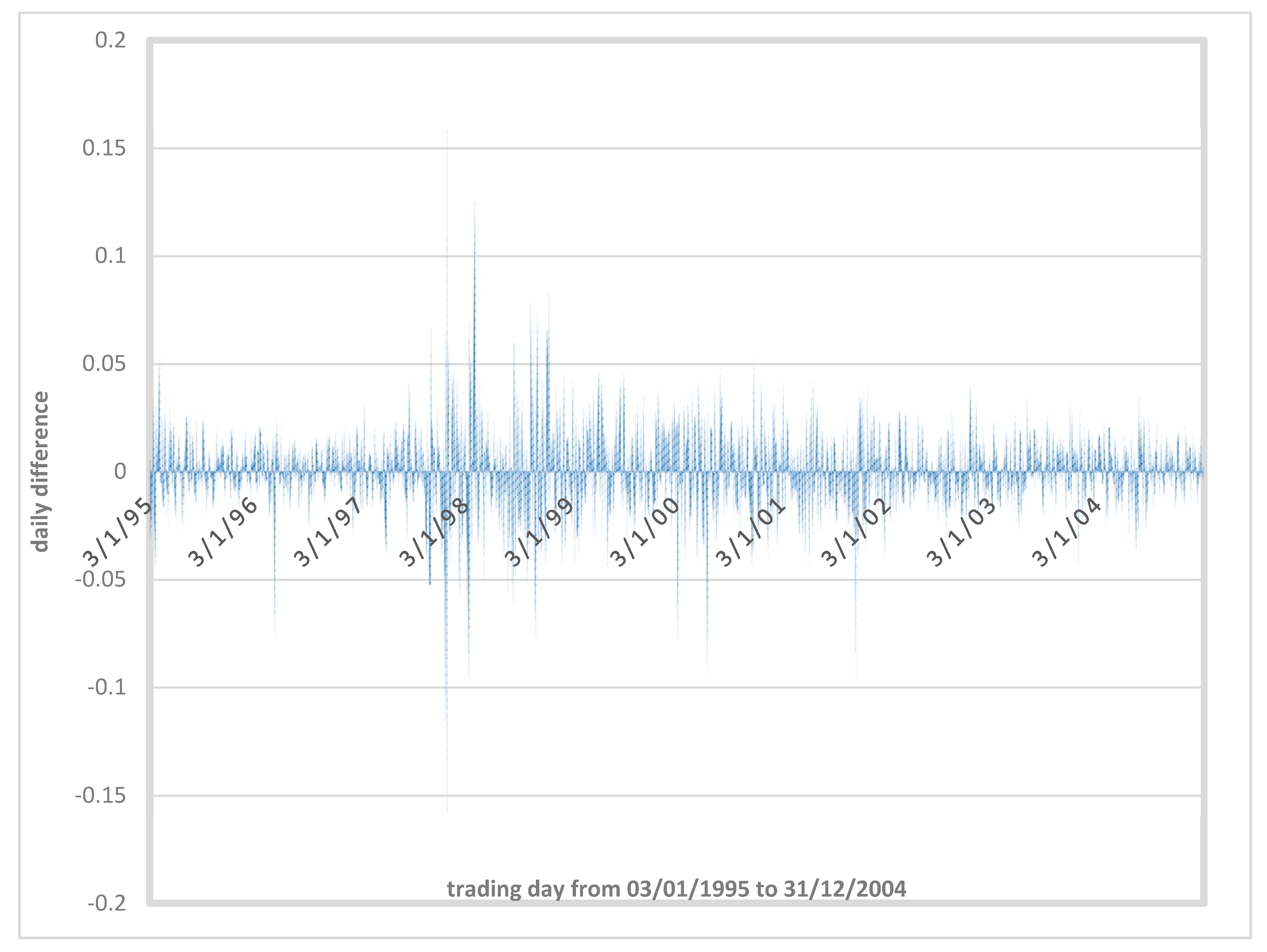
β represents the degree of influence of the F(t + 1) forecast based on the difference between the forecast stock index and the actual stock index. Moreover, given the volatility limitation of TAIEX (±7%) and the lack of a limit for the HSI stock, we plot the daily fluctuation of HSI as shown in Figure 2. From Figure 2, we see that the daily fluctuation is no greater than ±15%. Then, we can set the range of β from −0.15 to 0.15 to search for the optimal β.

(3)

γ represents the degree of influence of the F(t + 1) forecast from the daily difference of two stock indexes; the range of γ is [−1, 1], where −1 is an entire negative correlation, and 1 represents completely positive correlation.

In Equation (7), F(t) has been defuzzified by Equation (3) and M(L_VR(t)) has been transferred into the corresponding market signals by Equation (6). Therefore, the three factors have been crisp values, and the M(L_VR(t)) is an indicator signal; then M(L_VR(t)) × P(t) is a linear factor. Hence, the proposed model in Equation (7) is a linear multifactor forecasting model. Next, from Step 1 to Step 4, we employed the collected stock datasets to fit the Equation (7) based on the minimal RMSE to obtain the best parameters for α, β, and γ, and each iteration step is 0.001 for α, β, and γ, the detailed computation could be referred to Algorithm 1.

Step 6. Adapt the best parameters α, β, and γ.

To obtain the best parameters for α, β, and γ, the training data are used to adapt these parameters by calculating the minimum RMSE using Equation (8). We set a reasonable step iteration (here set as step = 0.001), thereby finally producing the best parameters for α, β, and γ.

$$\mathrm{RMSE}=\sqrt{\frac{{{\displaystyle \sum }}_{\mathrm{t}=1}^{\mathrm{n}}{\left|\mathrm{A}\left(t \right)-F\left(t \right)\right|}^2}{\mathrm{n}}}$$

(8)

where A(t) is the actual value on day(t), F(t) is the forecast value on day(t), and n is the number of trading days.

Step 7. Forecast the stock index.

In step 6, the parameters that optimize forecasting performance (minimum RMSE) are obtained in the training process. The trained Equation can then forecast F(t + 1) for the testing dataset.

Step 8. Evaluate the performance of the forecast.

Using Equation (8), the RMSE for all the testing data is calculated, and we use the RMSE as an evaluation criterion to compare with the listed models.

Algorithm 1: Multifactor FTS model

Input: double array ${\mathit{P}}_{\mathit{i}}$, ${\mathit{V}}_{\mathit{i}}$, ${\mathit{I}}_{\mathit{i}}$, ${\mathit{p}}_{\mathit{i}}$, ${\mathit{V}}_{\mathit{i}\mathbf{+}\mathit{h}}^{\mathit{t}}$, ${\mathit{I}}_{\mathit{i}\mathbf{+}\mathit{h}}^{\mathit{t}}$, and ${\mathit{p}}_{\mathit{i}\mathbf{+}\mathit{h}}^{\mathit{t}}$ begin   sum = 0   min RMSE = 999999999  // refer Equation (8)   for i←−150 to 150 do    for j←−150 to 150 do     for k←−1000 to 1000 do      for x←0 to length of factor1 do        forecast train $=\frac{i}{1000}\times {\mathit{P}}_{\mathit{i}}\left[x\right]+\frac{j}{1000}\times \mathit{f}\mathit{a}\mathit{c}\mathit{t}\mathit{o}\mathit{r}\mathbf{2}\left[x\right]+\frac{k}{1000}\times \mathit{f}\mathit{a}\mathit{c}\mathit{t}\mathit{o}\mathit{r}\mathbf{3}\left[x\right]+\mathit{D}\mathit{a}\mathit{t}\mathit{a}\mathbf{1}\left[x\right]$          // refer Equation (7), and set α = $\frac{i}{1000}$, β = $\frac{j}{1000}$, and γ = $\frac{k}{1000}$        square error $={\left(\mathit{D}\mathit{a}\mathit{t}\mathit{a}\mathbf{1}\left[x+1\right]-forecast\_train\right)}^2$        sum = sum + square error       end       if (min RMSE > RMSE)         best(i) = i         best(j) = j         best(k) = k         min RMSE = RMSE       end       RMSE = 0       square error = 0     end    end   end Output: best i, best j, best k

3.2. The Pseudocode of the Proposed Model

For easy computation, this section presents a pseudocode for the proposed model as Algorithm 1. The notation used in Algorithm 1 is introduced as follows:

${\mathit{P}}_{\mathit{i}}$:	stock index for training in the i-th year;
${\mathit{V}}_{\mathit{i}}$:	trading volume for training in the i-th year;
${\mathit{I}}_{\mathit{i}}$:	interaction between two stock markets for training in the i-th year;
${\mathit{p}}_{\mathit{i}}$:	closing price for training in the i-th year;
${\mathit{P}}_{\mathit{i}\mathbf{+}\mathit{h}}^{\mathit{t}}$:	next half-year stock index for testing in the i-th year;
${\mathit{V}}_{\mathit{i}\mathbf{+}\mathit{h}}^{\mathit{t}}$:	next half-year trading volume for testing in the i-th year;
${\mathit{I}}_{\mathit{i}\mathbf{+}\mathit{h}}^{\mathit{t}}$:	next half-year interaction between two stock markets for testing in the i-th year;
${\mathit{p}}_{\mathit{i}\mathbf{+}\mathit{h}}^{\mathit{t}}$:	next half-year closing price for testing in the i-th year.

4. Verification and Comparison

The TAIEX, HSI, and NASDAQ stock data from 1997 to 2004 are used as an experimental dataset in this study. Using the half-year sliding window method, we divide these dataset into fourteen overlapping sub-datasets. Each sub-dataset contains data covering one year for training and half a year for testing, and the window is shifted up by half a year for each sub-dataset. For verification, the forecast results of the fourteen TAIEX testing periods are listed in

Table 2. Forecast result for TAIEX testing data.

Training	Testing	α	β	γ	RMSE
1997/01~1997/12	1998/01~1998/06	−0.004	0.002	0.002	112
1997/07~1998/06	1998/07~1998/12	−0.006	0.005	0.002	104
1998/01~1998/12	1999/01~1999/06	−0.008	−0.001	0.002	97
1998/07~1999/06	1999/07~1999/12	−0.008	0.001	0.003	122
1999/01~1999/12	2000/01~2000/06	−0.009	0.049	0.003	168
1999/07~2000/06	2000/07~2000/12	0.0	0.057	−0.001	147
2000/01~2000/12	2001/01~2001/06	−0.006	−0.003	−0.002	94
2000/07~2001/06	2001/07~2001/12	−0.01	0.016	−0.003	91
2001/01~2001/12	2002/01~2002/06	−0.013	−0.003	0.001	98
2001/07~2002/06	2002/07~2002/12	−0.009	0.007	0.001	82
2002/01~2002/12	2003/01~2003/06	−0.005	0.024	0.0	71
2002/07~2003/06	2003/07~2003/12	−0.008	−0.002	0.002	61
2003/01~2003/12	2004/01~2004/06	−0.005	−0.01	0.003	112
2003/07~2004/06	2004/07~2004/12	−0.006	−0.004	0.002	59

and that the fourteen HSI testing periods in

Table 3. Forecast result for HSI testing data.

Training	Testing	α	β	γ	RMSE
1997/01~1997/12	1998/01~1998/06	−0.013	−0.021	−0.001	226
1997/07~1998/06	1998/07~1998/12	0.0	−0.07	−0.003	228
1998/01~1998/12	1999/01~1999/06	−0.019	0.024	−0.001	192
1998/07~1999/06	1999/07~1999/12	0.0	−0.014	0.002	208
1999/01~1999/12	2000/01~2000/06	−0.013	0.017	0.0	329
1999/07~2000/06	2000/07~2000/12	−0.014	0.041	−0.001	238
2000/01~2000/12	2001/01~2001/06	−0.016	0.065	−0.001	217
2000/07~2001/06	2001/07~2001/12	0.0	−0.015	−0.001	199
2001/01~2001/12	2002/01~2002/06	−0.01	0.013	0.0	116
2001/07~2002/06	2002/07~2002/12	−0.009	0.012	0.0	119
2002/01~2002/12	2003/01~2003/06	−0.008	−0.003	0.0	88
2002/07~2003/06	2003/07~2003/12	−0.009	0.017	0.001	115
2003/01~2003/12	2004/01~2004/06	0.0	0.006	0.001	153
2003/07~2004/06	2004/07~2004/12	−0.01	−0.017	0.0	106

.

To show the forecast results of the proposed model, we employed the RMSE as an evaluation indicator and used Chen’s [4], Huarng and Yu’s [9], and Chen et al.’s [7] FTS models as comparison models. To evaluate whether the performance of the proposed model surpassed that of conventional time series models, we also compared the performance of the proposed model with support vector regression [33] and a general regression neural network [34]. The experimental results for the TAIEX are shown in

Table 4. Forecast results of the TAIEX (six-month moving-window).

Testing	RMSE
	[4]	[9]	[7]	SVR	GRNN	Proposed
1998/01~1998/06	209	139	207	275	1208	112 a
1998/07~1998/12	339	160	361	393	1964	104 a
1999/01~1999/06	324	211	352	897	2381	97 a
1999/07~1999/12	195	162	205	919	1624	122 a
2000/01~2000/06	404	231	496	469	2508	168 a
2000/07~2000/12	319	293	563	742	4159	147 a
2001/01~2001/06	245	418	368	468	2813	94 a
2001/07~2001/12	368	823	536	441	2032	91 a
2002/01~2002/06	215	264	186	657	1797	98 a
2002/07~2002/12	155	237	157	672	2077	82 a
2003/01~2003/06	160	150	157	159	1582	71 a
2003/07~2003/12	150	459	246	733	1473	61 a
2004/01~2004/06	188	534	314	360	1924	112 a
2004/07~2004/12	106	166	96	392	1357	59 a
Average	241	303	303	541	2064	101a

^a The best performance among 6 models, SVR: support vector regression, and GRNN: general regression neural network.

and results for HSI are shown in

Table 5. Forecast results of the HSI (six-month moving-window).

Testing	RMSE
	[4]	[9]	[7]	SVR	GRNN	Proposed
1998/01~1998/06	620	491	1506	591	10192	226 a
1998/07~1998/12	434	294	776	251	3844	228 a
1999/01~1999/06	415	327	1197	758	6546	192 a
1999/07~1999/12	728	357	856	729	8309	208 a
2000/01~2000/06	678	460	924	353	5975	329 a
2000/07~2000/12	372	304	503	726	3703	238 a
2001/01~2001/06	589	466	662	504	4422	217 a
2001/07~2001/12	626	415	1099	994	9973	199 a
2002/01~2002/06	318	172	402	230	2761	116 a
2002/07~2002/12	232	192	225	496	3380	119 a
2003/01~2003/06	261	157	284	433	2091	88 a
2003/07~2003/12	325	256	329	509	7329	115 a
2004/01~2004/06	376	212	596	393	7913	153 a
2004/07~2004/12	313	159	262	119	2572	106 a
Average	449	304	687	506	5644	181a

Note: “a” denotes the best performance among the six models.

. These tables show that the proposed model outperformed the other models in the fourteen testing periods, and the average RMSE of Table 4 and Table 5 also shows that the proposed model outperformed the other models.

To test whether the proposed model outperforms the other models, we use a nonparametric Wilcoxon signed rank test [52] to compare all RMSEs of the two matched models and determine whether their population mean ranks are different. Each stock market has 15 pairwise comparisons (a pairwise comparison of six models), and the test results of two stock market are shown in

Table 6. Wilcoxon signed rank test for comparing proposed with listing methods.

TAIEX	[4]	[9]	[7]	SVR	GRNN
Proposed	+ *	+ *	+ *	+ *	+ *
GRNN	− *	− *	− *	− *
SVR	− *	− *	− *
[7]	− *	+
[9]	− *
HSI	[4]	[9]	[7]	SVR	GRNN
Proposed	+ *	+ *	+ *	+ *	+ *
GRNN	− *	− *	− *	− *
SVR	−	− *	+
[7]	− *	− *
[9]	+

Note: * denotes that a p-value less than 0.05 is statistically significant, “+” denotes the row method > column method, and “−” denotes the row method < column method.

. We see that all cells are “+ *” in the second and eighth row of Table 6, indicating that the proposed method is better than that of the other five models in the TAIEX and HSI datasets, and the GRNN presents the worst result.

5. Findings and Discussion

After verification and comparison, this section provides some findings and discusses the relevant problems. First, there are five findings:

(1)

From the literature review, the selected attributes (trading volume, stock index, and interaction between two stock markets) have been proved to have an impact on the forecast of the stock market, and the results have a minimal RMSE, which will lead to a higher profits for investors.

(2)

Table 4 and Table 5 indicate that the TAIEX is less volatile than the HSI. This is because Taiwan limits the volatility of shares to ±7%, whereas Hong Kong has no limit. From Figure 2, the daily fluctuation of HSI can help us to set the search range for quickly obtaining the optimal parameters for α and β.

(3)

As in Table 2, Taiwan is influenced by US stock market activity; the maximal impact γ is ±0.003. However, Table 3 shows that Hong Kong is less influenced by US stock market activity, and the impact γ is 0 in the five training periods.

(4)

From Table 2 and Table 3, the maximal parameter is β = 0.057 for TAIEX (1999/07~2000/06) and β = 0.065 for HSI (2000/01~2000/12). During this period (1999/07~2000/12), we searched “2000 crisis”. The results pertaining to the Dot-com bubble (2000–2002) and the year 2000 issues carry tremendous risks of disruption in the operations of financial institutions and in financial markets. Hence, we think that the “2000 crisis” has influenced the fluctuations of the stock market.

(5)

The comparative results (Table 4 and Table 5) and statistical test (Table 6) show that the proposed model outperforms other models in forecast accuracy (less RMSE) because the proposed linear multifactor forecasting equation with three optimized parameters (α, β, and γ) produces an optimal prediction to match past stock index patterns and generates a more accurate forecast.

From results and findings, we list three issues to discuss as follows:

(1) Will an accurate forecast lead to higher profits?

In general, the minimal forecast RMSE will lead to a higher profits for investors. However, it is very dangerous to directly use an AI forecast model for investing in the financial market. In practice, the use an AI forecast model has its limitations, such as factor selection (technical indicators, foundational analysis, and news), information quality, timely information, and investor policies (risk-adjusted trading strategy returns, valuable investment, short-term, very short-term, medium-to-long-term, and stock ownership), etc. Therefore, we suggest that the investors should be more cautious in using AI forecast models.

(2) How should one select a forecast model?

There are many algorithms we can use, from longstanding best practices to cutting-edge methodologies. Each algorithm has its pros and cons. The complexity, assumptions, and types of data inputs used in a given model type will vary, but the basic ingredients are similar across the board. Therefore, we suggest that a user first needs to understand the pros and cons of each model as a start, and the dataset would fit into a single model type. To understand the model limitations, it is also possible to build many forecast models to compare their performance.

(3) What are the advantages of using fuzzified historical data?

From the compared methods [4,7,9,33,34], we find that Chen method [4] is FTS model with one factor, Huarng and Yu [9] is also one factor with picking high (the highest price of the day) and low (the lowest price of the day) as Type 2 observations, and Chen et al. [7] is a one-factor FTS model with multi-period adaptation model. The three methods [4,7,9] are FTS models with simple and easy understanding, but they do not consider more key factors, hence their performance are not better than the proposed model. Furthermore, GRNN has local minimal point and over-fitting problems, and the computational requirement of the SVR is quite tedious [53], especially how to select the fitting kernel function is a key question.

6. Conclusions

This study proposed a novel multifactor FTS model based on stock volatility, the proposed model employs three crucial forecasting factors, namely, stock trading volume, stock index, and interaction between two stock markets. Experimental results for the TAIEX and HSI demonstrate that the proposed model forecasts the stock index effectively and outperforms other models in RMSE. From the forecast results of two stock markets, the average RMSE indicates that the proposed model outperformed the other models as shown in Table 4 and Table 5. However, HSI index has larger fluctuation than TAIEX index, because Taiwan stocks have a volatility limitation of ±7%, whereas HSI stocks have no such restriction. Hence, the larger fluctuation leads to the average RMSE of all models with larger RMSE except SVR in HSI dataset. On the other hand, the proposed model has the tolerance of fluctuation (smaller RMSE) as shown in Table 4 and Table 5.

After our findings and discussions, we found that the proposed model has three major advantages: (1) fuzzy time series with multifactor prediction; (2) to transform nonlinear model into linear fitting model with fast convergence and accurate forecast capability; and (3) from literature review, to select three important factors (stock index, trading volume, and the daily difference of two stock market indexes). Therefore, we think that the proposed model fits well into the current state of knowledge.

A simple and easy to explain model is the motivation of this study; therefore, we used three factors to build a linear combination of multifactor fuzzy time-series for forecasting stock index. From Ahmed and Khalid [53], we found the ANN-based forecasting models have some drawbacks such as local minimal point, over-fitting problems, etc. These drawbacks can be overcome by advanced hybrid intelligent models like SVM, ELM, and ANFIS. However, the computational requirement of most of these models is quite tedious, especially if training through an optimization technique is involved; this is a drawback for real applications. Hence, this study proposes a linear fitting model, which has been converted from a nonlinear fuzzy time-series multifactor model into a linear fitting model, and the proposed linear fitting model has fast convergence and accurate forecast capability.

Two suggestions to further enhance the proposed model by making its results less conservative and improving forecasting performance may be suggested: (1) Other forecast factors could be used in the proposed model; (2) other methods (such as machine learning algorithms) could be embedded in the proposed model, and (3) the policy of investor being a key factor to obtain profits, adding policies of investor could improve forecast capability and calculate the profits.

References

1. Song, Q.; Chissom, B.S. Forecasting enrollments with fuzzy time series—Part I. Fuzzy Sets Syst. 1993, 54, 1–9. [Google Scholar] [CrossRef]
2. Chen, S.-M.; Hsu, C.-C. A new method to forecast enrollments using fuzzy time series. Int. J. Appl. Sci. Eng. 2004, 2, 234–244. [Google Scholar] [CrossRef]
3. Chen, S.-M.; Wang, N.-Y.; Pan, J.-S. Forecasting enrollments using automatic clustering techniques and fuzzy logical relationships. Expert Syst. Appl. 2009, 36, 11070–11076. [Google Scholar] [CrossRef]
4. Chen, S.-M. Forecasting enrollments based on fuzzy time-series. Fuzzy Sets Syst. 1996, 81, 311–319. [Google Scholar] [CrossRef]
5. Chen, S.-M. Forecasting enrollments based on high-order fuzzy time series. Cybern. Syst. 2002, 33, 1–16. [Google Scholar] [CrossRef]
6. Yu, H.-K. Weighted fuzzy time-series models for TAIEX forecasting. Phys. A Stat. Mech. Its Appl. 2005, 349, 609–624. [Google Scholar] [CrossRef]
7. Chen, T.-L.; Cheng, C.-H.; Teoh, H.-J. High-order fuzzy time-series based on multi-period adaptation model for forecasting stock markets. Phys. A Stat. Mech. Its Appl. 2008, 387, 876–888. [Google Scholar] [CrossRef]
8. Hadavandi, E.; Shavandi, H.; Ghanbari, A. Integration of genetic fuzzy systems and artificial neural networks for stock price forecasting. Knowl.-Based Syst. 2010, 23, 800–808. [Google Scholar] [CrossRef]
9. Huarng, K.; Yu, H.-K. A type 2 fuzzy time series model for stock index forecasting. Phys. A Stat. Mech. Its Appl. 2005, 353, 445–462. [Google Scholar] [CrossRef]
10. Park, J.-I.; Lee, D.-J.; Song, C.-K.; Chun, M.-G. TAIFEX and KOSPI 200 forecasting based on two-factors high-order fuzzy time series and particle swarm optimization. Expert Syst. Appl. 2010, 37, 959–967. [Google Scholar] [CrossRef]
11. Chen, S.-M.; Hwang, J.-R. Temperature prediction using fuzzy time series. IEEE Trans. Syst. Man Cybern. Part B (Cybern.) 2000, 30, 263–275. [Google Scholar] [CrossRef] [PubMed] [Green Version]
12. Li, S.-T.; Kuo, S.-C.; Cheng, Y.-C.; Chen, C.-C. Deterministic vector long-term forecasting for fuzzy time series. Fuzzy Sets Syst. 2010, 161, 1852–1870. [Google Scholar] [CrossRef]
13. Cheng, C.-H.; Wei, L.-Y. Volatility model based on multi-stock index for TAIEX forecasting. Expert Syst. Appl. 2009, 36, 6187–6191. [Google Scholar] [CrossRef]
14. Lee, L.-W.; Wang, L.-H.; Chen, S.-M.; Leu, Y.-H. Handling forecasting problems based on two-factors high-order fuzzy time series. IEEE Trans. Fuzzy Syst. 2006, 14, 468–477. [Google Scholar] [CrossRef]
15. Dickinson, D.G. Stock market integration and macroeconomic fundamentals: An empirical analysis, 1980–1995. Appl. Financ. Econ. 2000, 10, 261–276. [Google Scholar] [CrossRef]
16. Kanas, A.; Yannopoulos, A. Comparing linear and nonlinear forecasts for stock returns. Int. Rev. Econ. Financ. 2001, 10, 383–398. [Google Scholar] [CrossRef]
17. Rashid, A. Stock prices and trading volume: An assessment for linear and nonlinear Granger causality. J. Asian Econ. 2007, 18, 595–612. [Google Scholar] [CrossRef]
18. Campbell, J.Y.; Grossman, S.J.; Wang, J. Trading volume and serial correlation in stock returns. Q. J. Econ. 1993, 108, 905–939. [Google Scholar] [CrossRef] [Green Version]
19. Chu, H.-H.; Chen, T.-L.; Cheng, C.-H.; Huang, C.-C. Fuzzy dual-factor time-series for stock index forecasting. Expert Syst. Appl. 2009, 36, 165–171. [Google Scholar] [CrossRef]
20. Hiemstra, C.; Jones, J.D. Testing for linear and nonlinear Granger causality in the stock price-volume relation. J. Financ. 1994, 49, 1639–1664. [Google Scholar] [CrossRef]
21. Kitt, R.; Kalda, J. Scaling analysis of multi-variate intermittent time-series. Phys. A Stat. Mech. Its Appl. 2005, 353, 480–492. [Google Scholar] [CrossRef] [Green Version]
22. Zhu, X.; Wang, H.; Xu, L.; Li, H. Predicting stock index increments by neural networks: The role of trading volume under different horizons. Expert Syst. Appl. 2008, 34, 3043–3054. [Google Scholar] [CrossRef]
23. Le, V.; Zurbruegg, R. The role of trading volume in volatility forecasting. J. Int. Financ. Mark. Inst. Money 2010, 20, 533–555. [Google Scholar] [CrossRef]
24. Wang, X.; Phua, P.K.H.; Lin, W. Stock market prediction using neural networks: Does trading volume help in short-term prediction? Proc. Int. Jt. Conf. Neural Netw. 2003, 4, 2438–2442. [Google Scholar] [CrossRef]
25. Su, C.-H.; Cheng, C.-H. A hybrid fuzzy time series model based on ANFIS and integrated nonlinear feature selection method for forecasting stock. Neurocomputing 2016, 205, 264–273. [Google Scholar] [CrossRef]
26. Stefanakos, C. Fuzzy time series forecasting of nonstationary wind and wave data. Ocean Eng. 2016, 121, 1–12. [Google Scholar] [CrossRef] [Green Version]
27. Zadeh, L.A. Fuzzy sets. Inf. Control 1965, 8, 338–353. [Google Scholar] [CrossRef] [Green Version]
28. Song, Q.; Chissom, B.S. Forecasting enrollments with fuzzy time series—Part II. Fuzzy Sets Syst. 1994, 62, 1–8. [Google Scholar] [CrossRef]
29. Bose, M.; Mali, K. Designing fuzzy time series forecasting models: A survey. Int. J. Approx. Reason. 2019, 111, 78–99. [Google Scholar] [CrossRef]
30. Chen, S.-M.; Zou, X.-Y.; Gunawan, G.C. Fuzzy time series forecasting based on proportions of intervals and particle swarm optimization techniques. Inf. Sci. 2019, 500, 127–139. [Google Scholar] [CrossRef]
31. Panigrahi, S.; Behera, H.S. A computationally efficient method for high order Fuzzy time series forecasting. J. Theor. Appl. Inf. Technol. 2018, 96, 7215–7226. [Google Scholar] [CrossRef]
32. Bas, E.; Grosan, C.; Egrioglu, E.; Yolcu, U. High order fuzzy time series method based on pi-sigma neural network. Eng. Appl. Artif. Intell. 2018, 72, 350–356. [Google Scholar] [CrossRef]
33. Avazbeigi, M.; Doulabi, S.H.H.; Karimi, B. Choosing the appropriate order in fuzzy time series: A new N-factor fuzzy time series for prediction of the auto industry production. Expert Syst. Appl. 2010, 37, 5630–5639. [Google Scholar] [CrossRef]
34. Vapnik, V.N. The Nature of Statistical Learning Theory; Springer: Berlin/Heidelberg, Germany, 2000. [Google Scholar]
35. Specht, D. F A general regression neural network. IEEE Trans. Neural Netw. 1991, 2, 568–576. [Google Scholar] [CrossRef] [PubMed] [Green Version]
36. Chen, C.-D.; Chen, S.-M. A New Method to Forecast the TAIEX Based on Fuzzy Time Series. In Proceedings of the 2009 IEEE International Conference on Systems, Man, and Cybernetics, San Antonio, TX, USA, 11–14 October 2009. [Google Scholar]
37. Huarng, K.-H.; Yu, T.H.-K.; Hsu, Y.W. A multivariate heuristic model for fuzzy time-series forecasting. IEEE Trans. Syst. Man Cybern. Part B Cybern. 2007, 37, 836–846. [Google Scholar] [CrossRef] [PubMed]
38. Tsai, I.-C. Dynamic price–volume causality in the American housing market: A signal of market conditions. North Am. J. Econ. Financ. 2019, 48, 385–400. [Google Scholar] [CrossRef]
39. Granger, C.W.J. Investigating causal relations by econometric models and cross-spectral methods. Econometrica 1969, 37, 424–438. [Google Scholar] [CrossRef]
40. Shen, C.-H.; Wang, L.-R. Daily serial correlation, trading volume and price limit: Evidence from the Taiwan stock market. Pac. Basin Financ. J. 1998, 6, 251–273. [Google Scholar] [CrossRef]
41. Bremer, M.; Hiraki, T. Volume and individual security returns on the Tokyo Stock Exchange. Pac. Basin Financ. J. 1999, 7, 351–370. [Google Scholar] [CrossRef]
42. Wang, C.; Chin, S. Profitability of return and volume-based investment strategies in China’s stock market. Pac. Basin Financ. J. 2004, 12, 541–564. [Google Scholar] [CrossRef]
43. Hodgson, A.; Masih, A.M.M.; Masih, R. Futures trading volume as a determinant of prices in different momentum phases. Int. Rev. Financ. Anal. 2006, 15, 68–85. [Google Scholar] [CrossRef]
44. Kim, M.-J.; Min, S.-H.; Han, I. An evolutionary approach to the combination of multiple classifiers to predict a stock price index. Expert Syst. Appl. 2006, 31, 241–247. [Google Scholar] [CrossRef]
45. Lee, B.-S.; Rui, O.M.; Wang, S.S. Information transmission between the NASDAQ and Asian second board markets. J. Bank. Financ. 2004, 28, 1637–1670. [Google Scholar] [CrossRef]
46. Yang, S.H. Dynamic Conditional Correlation Analysis of NASDAQ and Taiwan Stock Market. Master’s Thesis, Business Administration, National Chiao Tung University, Hsinchu, Taiwan, 2009. [Google Scholar]
47. Savva, C.S. International stock markets interactions and conditional correlations. J. Int. Financ. Mark. Inst. Money 2009, 19, 645–661. [Google Scholar] [CrossRef]
48. Kim, S.; In, F. The influence of foreign stock markets and macroeconomic news announcements on Australian financial markets. Pac. Basin Financ. J. 2002, 10, 571–582. [Google Scholar] [CrossRef]
49. Cheng, C.-H.; Liu, J.-W.; Lin, T.-H. Multi-factor fuzzy time series model based on stock volatility for forecasting Taiwan stock index. Adv. Mater. Res. 2011, 211–212, 1119–1123. [Google Scholar] [CrossRef]
50. Miller, G.A. The magical number seven, plus or minus two: Some limits on our capacity for processing information. Psychol. Rev. 1994, 63, 81–97. [Google Scholar] [CrossRef] [Green Version]
51. Cheng, C.-H.; Chen, T.-L.; Chiang, C.-H. Trend-weighted fuzzy time-series model for TAIEX forecasting. Lect. Note Comput. Sci. 2006, 4234, 469–477. [Google Scholar]
52. Wilcoxon, F. Individual comparisons by ranking methods. Biom. Bull. 1945, 1, 80–83. [Google Scholar] [CrossRef]
53. Ahmed, A.; Khalid, M. A review on the selected applications of forecasting models in renewable power systems. Renew. Sustain. Energy Rev. 2019, 100, 9–21. [Google Scholar] [CrossRef]
Figure 1. Procedure of the proposed model.
Symmetry 11 01474 g001
Figure 2. Daily fluctuation of HSI.
Symmetry 11 01474 g002