Article

Entropy Estimation of Inverse Weibull Distribution under Adaptive Type-II Progressive Hybrid Censoring Schemes

Department of Mathematics, Beijing Jiaotong University, Beijing 100044, China
*
Author to whom correspondence should be addressed.
Symmetry 2019, 11(12), 1463; https://doi.org/10.3390/sym11121463
Submission received: 31 October 2019 / Revised: 21 November 2019 / Accepted: 25 November 2019 / Published: 28 November 2019

Abstract

:
This paper discusses entropy estimations for two-parameter inverse Weibull distributions under adaptive type-II progressive hybrid censoring schemes. Estimations of entropy derived by maximum likelihood estimation method and Bayes estimation method are both considered. Different Bayes estimators using squared loss function, Linex loss function, general entropy loss function, and balanced loss function are derived. Numerical results are derived by Lindley’s approximation method. Especially, the interval estimation of entropy is derived through maximum likelihood estimation method. To test the effectiveness of the estimations, simulation studies are conducted. These entropy estimation methods are illustrated and applied to analyze a real data set.

1. Introduction

In the life testing field, different data collection models are created to simulate various realistic situations. Conventional censoring methods, type-I and type-II censoring schemes have evolved into progressive forms and have been explored and applied extensively.
Theoretically, these data sets take the unintentional loss of observed units into consideration, but in experiments, these conventional data sets are difficult to implement. Especially when the units work for a long time, it has been proved that the sample size of the type-I censored data set is usually small. At the same time, the progressive type-II censoring data set is difficult to realize as it may last for a long time.
Suppose the experimenter provides a time T, which is the ideal total test time, but they allow the experiment to last beyond it. If the number of failures that occur before time T reaches the expectation, the experiment will stop earlier than T. Otherwise, once the experimental time exceeds the time T, but the number of observed failures is still lower than m, we hope to terminate the experiment as soon as possible. In response to this expectation, the experimenter would prefer a design that ensures that m observed failure times are obtained to assure the efficiency of statistical inference while the total test time is not too far from the ideal time T. According to the basic characteristic of the censored sample, the smaller censored size, the shorter the experimental time. Therefore, if we want to terminate the experiment earlier while fixing sample size m, we should keep as many surviving items as possible in the test.
Introduced by the authors of [1], the adaptive type-II progressive hybrid censoring scheme was designed to satisfy such an expectation, thus reasonably and effectively shortening the experiment period. On the basis of the traditional type-II progressive censoring scheme, which removes some of the remaining individuals at each failure time, the adaptive type-II progressive hybrid actively adjusts the experimental time by responding to the experimenter’s expected duration of the experiment. It considers a traditional type-I censoring method that censors according to a specific time. Therefore, this kind of censoring scheme speeds up the experiment after the certain time T, improving the efficiency of the experiment.
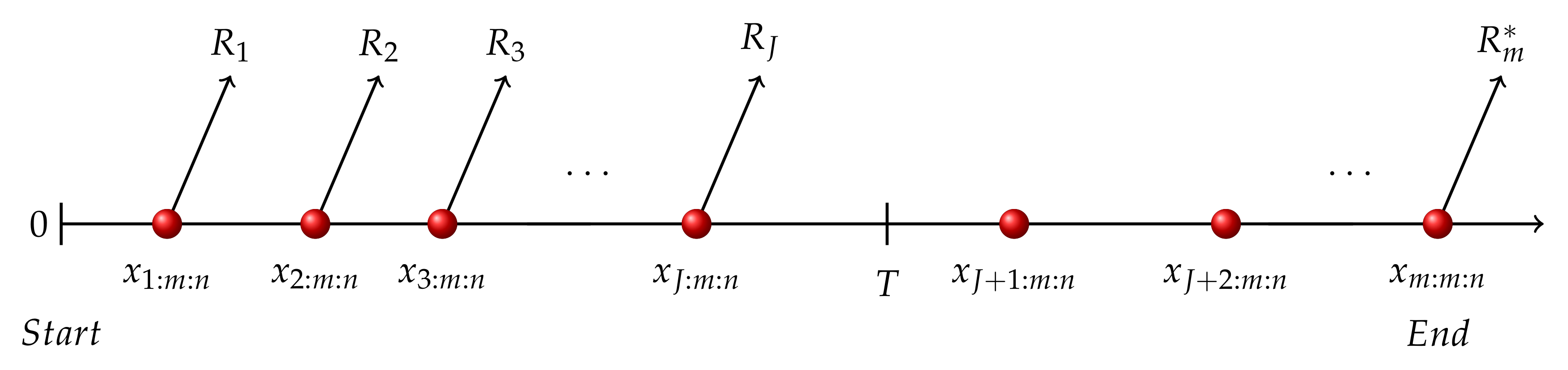
In this kind of data set, at each failure time x i : m : n , R i of remaining units will be removed. Although observed failures m and censored sample size are preset according to n and R 1 + R 2 + + R m + m = n , the censoring scheme R i varies depends on the performance of each individual and constraint time T. After setting threshold time T, appearances of adaptive type-II progressive hybrid censoring schemes under different cases depend on whether the m-th failure occurs beyond T (case I) or before T (case II).
In case I, see Figure 1, the m-th failure happens after certain time T and the last failure before time T occurs at x J : m : n , where J + 1 < m and x J : m : n < T < x J + 1 : m : n . In this situation, R J + 1 , R J + 2 , , R m 1 are set as R J + 1 = R J + 2 = = R m 1 = 0 , meanwhile R m = n m k = 1 J R k * .
In case II, see Figure 2, the m-th failure happens before time T. Therefore, adaptive type-II progressive hybrid censoring scheme degenerates into usual progressive type-II censoring data set, terminating at time x m : m : n .
Given the descriptions of these two schemes above, the likelihood functions of two cases can be written as
L I = K k = 1 m f ( x k : m : n ) k = 1 J [ 1 F ( x k : m : n ) ] R k [ 1 F ( x m : m : n ) ] R m * ,
L I I = K k = 1 m f ( x k : m : n ) [ 1 F ( x k : m : n ) ] R k .
where K = i = 1 m [ n i + 1 k = 1 max { i 1 , J } R k ] , R m * = n m k = 1 J R k .
Detailed in [2], one of the basic properties of order statistics is that the fewer operating items are withdrawn, the shorter total test time is expected. Thus, once the experiment lasts beyond expected time, the procedure will be accelerated. Through these changes, the experimenter can control the test time within a relatively short time interval without losing the number of observed failures.
Several distributions have been investigated under the adaptive type-II progressive hybrid censoring scheme. The authors of [3] compared estimations of parameters of generalized Pareto distribution and analyzed their creditable intervals using this kind of data samples. The authors of [1] contributed to computation of expected total test time and estimated failure rate for failure times under exponential distribution using this kind of data set. In addition, the authors of [4] estimated parameters, reliability functions, and hazard functions under adaptive type-II progressive hybrid censoring schemes for exponentiated Weibull distribution.
Inverse Weibull distribution plays an important role in reliability engineering and life testing, which was proposed to describe failures of mechanical components affected by degradation phenomenon. It has been investigated from various aspects. Reference [5] applied classical and Bayesian estimation procedures for estimations of parameters from Inverse Weibull distribution based on the progressive type-II censored data set. Especially considering Bayesian method, References [6] compared simulated risks of different estimators. References [7,8] devoted their efforts to its extensive versions investigations, including generalized inverse Weibull distribution as well as exponentiated generalized inverse Weibull distribution.
Inverse Weibull distribution has been explored from different perspectives. Many properties of this distribution are presented graphically and mathematically by [9], including variance and coefficients for variation, skewness, and kurtosis. Reference [10] estimated inverse Weibull distribution under a new prior distribution, including the considerations in the range of shape parameter and expected value of a quantile (reliable life) of the sampling distribution. Further extension of involving two inverse Weibull distributions into hybrid model was especially detailed in [11].
Obtaining a random variable x from inverse Weibull distribution, we display its cumulative distribution function and probability density function as
F ( x ; β , λ ) = exp ( λ x β ) β > 0 , λ > 0 , x > 0 ,
f ( x ; β , λ ) = β λ exp ( λ x β ) x ( β + 1 ) β > 0 , λ > 0 , x > 0 .
In which, shape parameter β and scale parameter λ ensure the flexibility and suitability of inverse Weibull distribution in numerous applications.
Nowadays, in the application field, the inverse Weibull distribution is still suitable for fitting numerous kinds of data resources. Depending on the value of the shape parameter, the hazard function of the inverse Weibull distribution can be reduced or increased. Therefore, the inverse Weibull distribution model is more appropriate in many conditions. The superiority of this distribution in providing a satisfactory parameter fit is often emphasized in articles when the nonmonotonic and unimodal hazard rate functions are strongly indicated in the data set. Reference [12] established analysis models for the first-order reaction of lignocellulosic biomass through inverse Weibull distribution. Regardless of various pre-exponential factors and activation energies, inverse Weibull distributions perform better in reaction sequences description. Reference [13] preferred the hybrid model based on inverse Weibull distribution to analyze the capacity of a cellular network in a cellular system employing multi-input multi-output beam-forming in rich and limited scattering environments. Such wide applications of inverse Weibull distribution are attributed to its flexible scale and shape parameters.
Entropy, raised by Shannon during investigation on communication (see [14]), constitutes the framework of information theory. The well-known Shannon entropy pioneers the information measurement field and has been widely used and studied today. This entropy of lifetime distribution can be calculated through
H ( f ) = 0 f ( x ) ln f ( x ) d x .
Entropy describes the uncertainty expressed by probability density function. Various distributions have different entropy values, describing distributions from another perspective and grabbing extensive attention to it. However, only numerical description of the entropy can be used to improve the practical experiments. Therefore, its calculation and estimation of different distributions are important. Reference [15], focused on entropy estimations of multivariate normal distribution. Reference [16] discussed estimations of Rayleigh distribution against criteria of bias, root mean squared error and Kullback–Leibler divergence values. Also, the authors of [17] contributed to the entropy estimations of Weibull distribution using generalized progressive hybrid censored samples.
Using inverse Weibull distribution, we derive the Shannon entropy of it directly from Equations (4) and (5) as follows.
H ( f ) = γ + β + γ β β ln β + ln λ β ,
where γ denotes the Euler–Mascheroni constant γ = 0.5772
In this paper, we focus on the entropy estimation of inverse Weibull distribution when samples derived under adaptive type-II progressive hybrid censoring schemes. Maximum likelihood estimation and Bayes estimation with multiple loss functions are studied.
The rest of the article is organized as follows. In Section 2, maximum likelihood estimations in different cases are obtained, including point estimation and approximate confidence interval estimation. Then, in Section 3, Bayes estimations of entropy are also proposed. Three loss functions and their balanced extension are considered. Lindley’s approximation method is used for calculation of Bayesian estimates. Through Monte Carlo simulation, in Section 4, we present comparisons of different estimators in tables and figures. In Section 5, a real data set is applied for illustrative purposes. Finally, Section 6 summarizes with a short conclusion.

2. Maximum Likelihood Estimation

Using general likelihood functions (1) and (2), and functions of inverse Weibull distribution, the likelihood functions of the censored sample are given by
  • Case I
    L I ( β , λ ) = K ( β λ ) m [ 1 exp ( λ x k : m : n β ) ] R m * k = 1 m x k : m : n ( β + 1 ) exp ( λ x k : m : n β ) k = 1 J [ 1 exp ( λ x k : m : n β ) ] R k .
  • Case II
    L I I ( β , λ ) = K ( β λ ) m k = 1 m exp ( λ x k : m : n β ) x k : m : n ( β + 1 ) [ 1 exp ( λ x k : m : n β ) ] R k .
When considering various schemes, likelihood functions can be written as an expression with different coefficients.
L c ( β , λ ) = K ( β λ ) m k = 1 m exp ( λ x k : m : n β ) x k : m : n ( β + 1 ) [ 1 exp ( λ x k : m : n β ) ] R k c
where K = i = 1 m [ n i + 1 k = 1 max { i 1 , j } R k c ] and c = 1 , 2 denotes different cases, within which schemes have different appearances beyond R J .
In case I, c = 1 , R m 1 = n J k = 1 J R k 1 , and R J + 1 1 = R J + 2 1 = = R m 1 1 = 0 are also required besides the prerequisite R 1 + R 2 + + R m + m = n .
In case II, c = 2 and R k 2 (where k > J ) can be defined randomly as long as they meet the sum requirement.
Therefore, the log-likelihood function is
l c ( β , λ ) m ln ( β λ ) k = 1 m λ x k : m : n β ( β + 1 ) k = 1 m ln ( x k : m : n ) + k = 1 m R k c ln [ 1 exp ( λ x k : m : n β ) ] .
The corresponding score equations are
l c ( β , λ ) λ = m λ k = 1 m x k : m : n β k = 1 m R k c x k : m : n β u k = 0 ,
l c ( β , λ ) β = m β + λ k = 1 m x k : m : n β ln ( x k : m : n ) k = 1 m ln ( x k : m : n ) λ k = 1 m R k c x k : m : n β u k ln ( x k : m : n ) = 0 .
where u k = exp ( λ x k : m : n β ) [ 1 exp ( λ x k : m : n β ) ] 1 .

2.1. Point Estimation of Entropy

However, it is difficult to derive explicit numerical solutions using Equations (11) and (12). Thus, a numerical method should be used to figure out the values.
To begin with, through transformations, we obtain functional expressions of λ ^ and β ^ through
λ ^ ( β ) = m k = 1 m x k : m : n β [ 1 + R k c u k ] ,
β ^ = h ( β ) = m λ ^ ( β ) k = 1 m x k : m : n β ln ( x k : m : n ) [ 1 R k c u k ] k = 1 m ln ( x k : m : n ) .
Having the initial guess, β ( 0 ) , we assume β ( 1 ) = h ( β ( 0 ) ) . Following such recurrence, a sequence of β ( i ) as β ( i ) = h ( β ( i 1 ) is produced. Stop the procedure once | β ( i ) β ( i 1 ) | < ϵ , where ϵ is a preset tolerance. Taking β ( i ) as the estimated value β ^ , we derive λ ^ as the estimation of λ as well. Once we have β ^ and λ ^ , the maximum likelihood estimation of entropy can be easily derived as
H ^ ( f ) = γ + β ^ + γ β ^ β ^ ln β ^ + ln λ ^ β ^ .

2.2. Approximate Confidence Intervals of Entropy

In statistics, the delta method is the result of an approximate probability distribution of the asymptotic normal statistical estimator function from the limit variance of the estimator. This method is well known for its generality in deriving the variances and approximate confidence intervals of estimators by creating a linear approximation of maximum likelihood function. Reference [18] used the Delta method for estimation of new Weibull–Pareto distribution based on progressive Type-II censored sample. Reference [19] also used this method for estimation of the two-parameter bathtub lifetime model. Different loss functions for Bayes estimation are considered and realized through Monte Carlo method.
In this section, the Delta method is used to derive the confidence intervals of entropy H ( f ) in the following Algorithm 1.
In Algorithm, D is calculated through
H ( f ) β = 1 β γ + ln λ β 2 , H ( f ) λ = 1 β λ
Algorithm 1. Entropy estimation using Delta method.
1:
Derive vector D as
D = H ( f ) β , H ( f ) λ β = β ^ , β = λ ^ .
2:
Calculate estimated variance of H ^ ( f ) as
V ( H ^ ( f ) ) = [ D I c 1 ( β , λ ) D T ] ,
where D T is the transpose of matrix D.
3:
Calculate the approximate confidence interval of H ^ ( f ) .
H ^ ( f ) z θ / 2 V ( H ^ ( f ) ) , H ^ ( f ) + z θ / 2 V ( H ^ ( f ) )
I 1 ( β , λ ) denotes the Fisher information matrix of the parameters, which could be further calculated through the derivation in Equations (11) and (12).
I c ( β ^ , λ ^ ) = I 11 I 12 I 21 I 22
I 11 = l c ( X ˜ | β , λ ) β 2 = m β 2 + λ k = 1 m x k : m : n β [ ln ( x k : m : n ) ] 2 λ k = 1 m R k c x k : m : n β u k [ ln ( x k : m : n ) ] 2 + λ k = 1 m R k c x k : m : n β u k β ln ( x k : m : n ) .
I 12 = l c ( X ˜ | β , λ ) β λ = k = 1 m x k : m : n β ln ( x k : m : n ) k = 1 m R k c x k : m : n β u k ln ( x k : m : n ) + λ k = 1 m R k c x k : m : n β u k λ ln ( x k : m : n )
I 21 = l c ( X ˜ | β , λ ) λ β = k = 1 m x k : m : n β ln ( x k : m : n ) k = 1 m R k c x k : m : n β u k ln ( x k : m : n )
k = 1 m R k c x k : m : n β u k β ln ( x k : m : n )
I 22 = l c ( X ˜ | β , λ ) λ 2 = m λ 2 k = 1 m R k c x k : m : n β u k λ
Within which the u k β and u k λ represent the partial derivatives of equation u k for β and λ , respectively.
u k β = λ exp ( 2 λ x k : m : n β ) ln ( x k : m : n ) x k : m : n β [ exp ( λ x k : m : n β ) 1 ] 2 λ exp ( λ x k : m : n β ) ln ( x k : m : n ) x k : m : n β [ exp ( λ / x k : m : n β ) 1 ]
u k λ = exp ( λ x k : m : n β ) x k : m : n β [ exp ( λ x k : m : n β ) 1 ] exp ( 2 λ x k : m : n β ) x k : m : n β [ exp ( λ x k : m : n β ) 1 ] 2

3. Bayes Estimations

The Bayesian method provides a solution to derive the estimation of certain distribution based on the prior information and the sample information. Prior information is processed into prior distribution. Therefore, it can be combined with likelihood function to derive posterior distribution. During this process, different estimators are evaluated through loss functions, which determine the criterion for selecting the optimal estimator.
Prior distribution is an important factor in Bayes estimation since its influence cannot be completely eliminated. In this paper, Gamma distributions are prior distributions for parameters β and λ of inverse Weibull distribution. We assume that β follows Gamma distribution with hyperparameters ( s , t ) , meanwhile λ follows the Gamma distribution with hyperparameters ( a , b ) . Thus, their joint prior distribution can be derived directly.
π ( β , λ ) β s 1 exp ( t β ) λ a 1 exp ( b λ )
Based on Equation (9), the joint prior distribution of β , λ , and X ˜ = ( x 1 : m : n , , x m : m : n ) is
π ( β , λ , X ˜ ) β s 1 exp ( t β ) λ a 1 exp ( b λ ) ( β λ ) m k = 1 m exp ( λ x k : m : n β ) x k : m : n ( β + 1 ) [ 1 exp ( λ x k : m : n β ) ] R k c .
Given X ˜ , the posterior distribution of β and λ is apparently.
π ( β , λ | X ˜ ) π ( β , λ , X ˜ ) 0 0 π ( β , λ , X ˜ ) d β d λ
In this section, we first use squared error loss function, Linex loss function, and general entropy loss function to carry out Bayes estimations of inverse Weibull distribution under Gamma prior distribution. On this basis, balanced loss function is also considered to promote the estimation. Then, we use Lindley’s approximation to calculate results.

3.1. Three Loss Functions

The loss function determines the choosing of best estimator to a certain degree. In this section, we consider three different loss functions and derive their estimation results of entropy for comparing different Bayes estimations.

3.1.1. Squared Error Loss Function

Squared error loss (SEL) function is applicable when considering symmetric loss functions. The loss function is shown as
L S ( ϕ , σ ) = ( ϕ σ ) 2 ,
where ϕ is the estimation of parameter σ .
Therefore, under the squared error loss function, the Bayes estimates can be obtained theoretically as
H ˜ S ( f ) = 0 H ( f ) π ( β , λ , X ˜ ) d β d λ 0 0 π ( β , λ , X ˜ ) d β d λ .

3.1.2. Linex Loss Function

The Linex loss function is applied when considering asymmetric loss functions. It plays an important role in engineering evaluation when positive and negative errors have unequal influence on the estimation. On the basis of discussions given in [20], the Linex loss function is shown as
L L ( ϕ , σ ) = exp ( h ( σ ϕ ) ) h ( σ ϕ ) 1 , h 0 .
The constant h denotes the weight of errors on different directions. If h > 0 , the positive errors are more serious than negative ones. If h < 0 , the lower estimations are more significant than higher estimations. If h is close to 0, the Linex loss function is close to squared loss function.
The Bayes estimator using the Linex loss function is described as
ϕ ^ L = 1 h ln [ E ϕ ( exp ( h ϕ ) | X ) ] .
Therefore, under the Linex loss function, Bayes estimates can be obtained theoretically as
H ˜ L ( f ) = 1 h ln [ 0 exp ( h H ( f ) ) π ( β , λ , X ˜ ) d β d λ 0 0 π ( β , λ , X ˜ ) d β d λ ] .

3.1.3. General Entropy Loss Function

General entropy loss function is also a widely used asymmetric loss function introduced in [21] and extended in [22]. Endowing flexibility to location parameter and scale parameter in measurement, this modified Linex function is also popular in lots of fields. The general entropy loss function is shown as
L E ( ϕ , σ ) ( σ ϕ ) q q ln ( σ ϕ ) 1 , q 0 .
The constant q also denotes how much influence that an error will have. If q > 0 , positive errors cause more serious consequences than negative ones. On the other hand, if q < 0 , negative errors affect the consequences more seriously.
The Bayes estimator using General entropy loss function is described as
ϕ ^ E = [ E ϕ ( ϕ q | X ) ] 1 / q .
Therefore, under the general entropy loss function, Bayes estimates can be obtained theoretically as
H ˜ E ( f ) = [ 0 H ( f ) q π ( β , λ , X ˜ ) d β d λ 0 0 π ( β , λ , X ˜ ) d β d λ ] 1 / q .

3.2. Bayes Estimation Using Balanced Loss Function

Based on the different loss functions, general balanced loss function gives out an uniform expression of different Bayes estimates. Such loss function is in the form of
L ρ , w , σ 0 ( ϕ , σ ) = w ρ ( σ 0 , σ ) + ( 1 w ) ρ ( ϕ , σ ) ,
where ρ is a general expression of any conventional loss function and σ 0 is a target estimator of σ .
With transformations of expression in balanced loss function, all the estimators mentioned above, including maximum likelihood estimation, symmetric, and asymmetric Bayes estimation, can be presented as special cases. When ρ denotes different functions, such as ( ϕ σ ) 2 , exp ( h ( σ ϕ ) ) h ( σ ϕ ) 1 , or ( σ ϕ ) q q ln ( σ ϕ ) 1 , function (33) describes the squared error estimation, Linex loss function, and general entropy loss function.
In addition, through different values of w, the balanced loss function reflects the proximity of estimation towards target estimator σ 0 or unknown parameter ϕ . Thus, this loss function is more general, as artificial preferences can be attached to this kind of function. Wide applications of it can be detected through [23,24].
According to [17], the approximate Bayes estimations based on the balanced loss functions are given as
H ^ B S ( f ) = w H ^ ( f ) + ( 1 w ) H ^ s ( f ) ,
H ^ B L ( f ) = 1 h ln [ w exp [ h H ^ ( f ) ] + ( 1 w ) exp [ h H ^ L ( f ) ] ] ,
H ^ B E ( f ) = [ w H ^ q ( f ) + ( 1 w ) H ^ E q ( f ) ] 1 / q .

3.3. Lindley’s Approximation

All the initial appearances of Bayes estimation above are ratio of two integrals which are not feasible to obtain the explicit results directly. Therefore, Lindley’s approximation is used to figure out the numerical solutions. This method has been used extensively (see [25,26]) as it gives out numerical result through simplifying transformation.
In the two-parameter case, according to the authors of [17], Lindley’s approximation is written as
L ^ B ( θ ) = 1 2 ( Q + y 30 S 12 + y 03 S 21 + y 21 P 12 + y 12 P 21 ) + p 1 Q 12 + p 2 Q 21 + L ^ ( θ ) ,
where τ i j denotes the ( i , j ) -th element of the matrix [ 2 l / θ 1 i θ 2 j ] 1 , l denotes the log-likelihood function, and
Q = i = 1 2 j = 1 2 u i j τ i j , Q i j = u i τ i i + u j τ j i , S i j = ( u i τ i i + u j τ i j ) τ i i , P i j = 3 u i τ i i τ i j + u j ( τ i i τ j j + 2 τ i j 2 ) , y i j = l ( θ 1 , θ 2 ) θ 1 i θ 2 j , p i = p θ i , u i = L ^ ( θ ) θ i , u i j = L ^ ( θ ) θ i θ j , p = ln π ( θ 1 , θ 2 ) , i , j = 0 , 1 , 2 , 3 .
Based on these equations, we can calculate the Lindley’s approximation of entropy estimation of inverse Weibull distribution:
y 30 = 3 l β 3 = 2 m β 3 λ k = 1 m x k : m : n β ( ln ( x k : m : n ) ) 3 λ k = 1 m R k c u k x β ( ln ( x k : m : n ) ) 3 2 λ k = 1 m R k c u k β x β ( ln ( x k : m : n ) ) 2 λ k = 1 m R k c u k β x β ( ln ( x k : m : n ) )
y 21 = 3 l β 2 λ = k = 0 m x k : m : n β ( ln ( x k : m : n ) ) 2 k = 1 m R k c u j x β ( ln ( x k : m : n ) ) 2 k = 1 m R j c u k λ x β ( ln ( x k : m : n ) ) 2 k = 1 m R k c u j x β ( ln ( x k : m : n ) ) λ k = 1 m R k c u k β λ x β ( ln ( x k : m : n ) )
y 20 = 2 l β 2 = m β 2 λ k = 1 m x k : m : n β ( ln ( x k : m : n ) ) 2 λ k = 1 m R k c u k x k : m : n β ( ln ( x k : m : n ) ) 2 λ k = 1 m R k c u k β x k : m : n β ln ( x k : m : n )
y 11 = 2 l β λ = k = 1 m x k : m : n β ln ( x k : m : n ) k = 1 m R k c u k x k : m : n β ln ( x k : m : n ) λ k = 1 m R k c u k λ x k : m : n β ln ( x k : m : n )
y 12 = 3 l β λ 2 = k = 1 m R k c u k λ x k : m : n β ln ( x k : m : n ) k = 1 m R k c u k λ x k : m : n β ln ( x k : m : n ) λ k = 1 m R k c u k λ x k : m : n β ln ( x k : m : n )
y 03 = 3 l λ 3 = 2 m λ k = 1 m x k : m : n β u k λ y 02 = 2 l λ 2 = m λ 2 k = 1 m x k : m : n β u k λ
τ 11 = y 02 y 20 y 02 y 11 2 τ 22 = y 20 y 20 y 02 y 11 2 τ 12 = τ 21 = y 11 y 20 y 02 y 11 2
u k β and u k β are first and second derivative of u k by β , respectively; also, u k λ and u k λ are the first and second derivative of u k by λ , respectively. For convenience of illustration, we display u k β .
u j β = 3 λ 2 exp ( 2 λ x k : m : n β ) ( ln ( x k : m : n ) ) 2 x k : m : n ( 2 β ) ( exp ( λ x k : m : n β ) 1 ) 2 λ 2 exp ( λ x k : m : n β ) ( ln ( x k : m : n ) ) 2 x k : m : n 2 β ( exp ( λ x k : m : n β ) 1 ) 2 λ 2 exp ( 3 λ x k : m : n β ) ( ln ( x k : m : n ) ) 2 x k : m : n 2 β ( exp ( λ x k : m : n β ) 1 ) 3 + λ exp ( λ x k : m : n β ) ( ln ( x k : m : n ) ) 2 ( x k : m : n β ( exp ( λ x k : m : n β ) 1 ) ) λ exp ( 2 λ x k : m : n β ) ( ln ( x k : m : n ) ) 2 x k : m : n β ( exp ( λ x k : m : n β ) 1 ) 2
Using the Lindley’s approximation shown above, we can calculate the approximation results of Bayes estimates against different loss functions.
Under the squared error loss function,
L ( β , λ ) = H ( f ) = γ + β + γ β β ln β + ln λ β .
u 1 = L β = γ β 2 1 β ln λ β 2 u 2 = L λ = 1 λ β u 22 = 2 L λ 2 = 1 λ 2 β u 21 = u 12 = 2 L β λ = 1 λ β 2 u 11 = 2 L β 2 = 2 ( γ + ln λ ) β 3 + 1 β 2
Using Equation (37), the approximate Bayes estimation H ^ S ( f ) can be derived as
H ^ S ( f ) = H ^ ( f ) + 0.5 [ l 30 ( u 1 τ 11 + u 2 τ 12 ) τ 11 + l 03 ( u 2 τ 22 + u 1 τ 21 ) τ 22 + l 21 { 3 u 1 τ 11 τ 12 + u 2 ( τ 11 τ 22 + 2 τ 12 2 ) } + ( u 11 τ 11 + 2 u 12 τ 12 + u 22 τ 22 ) ] + p 1 ( u 1 τ 11 + u 2 τ 21 ) + p 2 ( u 2 τ 22 + u 1 τ 12 ) .
Under the Linex loss function,
L ( β , λ ) = exp [ h H ( f ) ] = exp [ h ( γ + β + γ β β ln β + ln λ β ) ] .
u 1 = L β = h [ γ β 2 1 β ln λ β 2 ] exp [ h H ( f ) ]    u 2 = L λ = h λ β exp [ h H ( f ) ] u 11 = 2 L β 2 = h { 2 γ β 3 + 1 β 2 + 2 ln λ β 3 h [ γ β 2 1 β ln λ β 2 ] 2 } exp [ h H ( f ) ] u 21 = u 12 = 2 L β λ = h λ β 2 exp [ h H ( f ) ] + h 2 λ β [ γ β 2 1 β ln λ β 2 ] exp [ h H ( f ) ] u 22 = 2 L λ 2 = h λ β exp [ h H ( f ) ] [ h λ β 1 λ ]
Using Equation (37), the approximate Bayes estimation H ^ L ( f ) can be derived as
H ^ L ( f ) = 1 h ln { exp [ h H ^ ( f ) ] + 0.5 [ l 30 ( u 1 τ 11 + u 2 τ 12 ) τ 11 + l 03 ( u 2 τ 22 + u 1 τ 21 ) τ 22 + l 21 { 3 u 1 τ 11 τ 12 + u 2 ( τ 11 τ 22 + 2 τ 12 2 ) } + ( u 11 τ 11 + 2 u 12 τ 12 + u 22 τ 22 ) ] + p 1 ( u 1 τ 11 + u 2 τ 21 ) + p 2 ( u 2 τ 22 + u 1 τ 12 ) } .
Under the general entropy loss function,
L ( β , λ ) = [ H ( f ) ] q = ( γ + β + γ β β ln β + ln λ β ) q .
u 1 = L β = q ( γ β 2 1 β ln λ β 2 ) H ( q + 1 ) ( f )    u 2 = L λ = q ( 1 λ β ) H ( q + 1 ) ( f ) u 21 = u 12 = 2 L β λ = q ( 1 λ β ) H ( q + 2 ) ( f ) [ 1 β H ( f ) ( q + 1 ) ( γ β 2 1 β ln λ β 2 ) ] u 11 = 2 L β 2 = q H ( q + 2 ) ( f ) [ ( 2 γ β 3 + 1 β 2 + 2 ln λ β 3 ) H ( f ) ( q + 1 ) ( γ β 2 1 β ln λ β 2 ) 2 ] u 22 = 2 L λ 2 = q ( 1 λ β ) H ( q + 2 ) [ 1 λ H ( f ) + ( q + 1 ) ( 1 λ β ) ]
Using Equation (37), the approximate Bayes estimation H ^ E ( f ) can be derived as
H ^ E ( f ) = [ H ^ ( f ) q + 0.5 [ l 30 ( u 1 τ 11 + u 2 τ 12 ) τ 11 + l 03 ( u 2 τ 22 + u 1 τ 21 ) τ 22 + l 21 { 3 u 1 τ 11 τ 12 + u 2 ( τ 11 τ 22 + 2 τ 12 2 ) } + ( u 11 τ 11 + 2 u 12 τ 12 + u 22 τ 22 ) ] + p 1 ( u 1 τ 11 + u 2 τ 21 ) + p 2 ( u 2 τ 22 + u 1 τ 12 ) ] 1 / q .

4. Simulation Results

Monte Carlo method is an important procedure of statistical analysis that provides a certain method for simulation through generating random variables under a certain distribution. In this section, we compare the performances of different estimations using this method.
At the beginning, we derive Algorithm 2 to generate adaptive type-II progressive hybrid censored sample under inverse Weibull distribution following the method proposed in [1].
Algorithm 2 Generating adaptive type-II progressive hybrid censoring data under inverse Weibull distribution.
1:
For each i ∈ [1,m], generate W i following uniform distribution.
2:
For each i ∈ [1,m], generate V i : m : n through relationship with R i and W i as
V 1 = W 1 1 / 1 + R m ,
V 2 = W 2 1 / ( 2 + R m + R m 1 ) ,
,
V m = W m 1 / ( m + R m + R m 1 + + R 1 ) .
3:
For each i ∈ [1,m], generate U i : m : n through relationship with V i as
U 1 = 1 V m ,
U 2 = 1 V m V m 1 ,
,
U m = 1 V m V m 1 V 1 .
4:
For each i ∈ [1,m], derive x 1 : m : n , x 2 : m : n , , x m : m : n following x i : m : n = F 1 ( U i ) ,
where F 1 denotes the inverse Weibull distribution’s inverse cumulative functional expression
with parameters ( β , λ ).( i = 1 , 2 , , m )
5:
When X J : m : n < T < X J + 1 : m : n , set index J and record X 1 : m : n , , X J + 1 : m : n
6:
Record X J + 2 : m : n , , X m : m : n , as first m J 1 order statistics following truncated distribution f ( x ) / [ 1 F ( x J + 1 ) ] with sample size ( n J 1 k = 1 J R j c ) .
Without loss of generality, we set parameters of the inverse Weibull distribution to β = λ = 1 .
Next, we create adaptive type-II progressive hybrid censoring schemes by setting the schemes and threshold time T. It is used to display the estimation appearances under different cases of adaptive type-II progressive hybrid censoring data set. Therefore, we take different T into consideration by setting them to T = 0.7 , 1.5 , respectively.
Meanwhile, this paper also considers various adaptive type-II progressive hybrid censored data set through three kinds of censoring schemes. Schemes themselves have different versions in case I and case II. However, for illustration convenience, they are displayed in Table 1. As the proportions of the censored samples and observed samples also influence the entropy values, various m and n are set to n = 30 , 40 , 60 , m = 10 , 15 . Also, to avoid over censoring, we chose s = 1 when n = 30 , 40 , while s = 3 when n = 60 .
Finally, in the computation of each estimation, we use noninformative prior distribution with parameters h and q set to h = 1.5 , 0.5 , 1 (for Linex loss function); q = 1.5 , 0.5 , 1 (for general entropy loss function); and w = 0.2 , 0.5 , 0.8 (for balanced loss function).
In interval estimation, we derive the variances of estimated entropy, indicating the approximate interval of entropy of different progressive type-II censoring schemes. Under different conditions, the lengths of estimation interval are tabulated in Table 2.
According to results, it is reasonable to assume that the censoring pattern, the censored size, and the time limitation T are apparently related to the interval estimation.
  • With the growth of time constraint T, the lengths of approximate confidence intervals of entropy decrease.
  • When observed failure amount increases while sample size is fixed, the lengths of approximate confidence intervals of entropy decrease.
  • Censoring scheme c. usually leads to shorter estimation intervals.
In point estimation, following the method for computation using descriptions of β ^ and λ ^ as in Equations (13) and (14), we derive the estimates under maximum likelihood estimations method and Bayes estimation methods against squared error loss function, Linex loss function, and general entropy loss function. According to discussions in Section 3, balanced loss function-based estimations against three loss functions above are also calculated through Lindley’s approximation. Using Monte Carlo method, we replicate the procedures 1000 times in each case to present the comparisons. All the estimations are compared by presenting their mean squared error (MSE) (units is 0.1) and bias (units is 0.1) in Table 3, Table 4, Table 5, Table 6, Table 7, Table 8, Table 9 and Table 10.
As can be seen from tables, the properties of the estimates under all of the above conditions are as follows.
  • All the maximum likelihood estimates and Bayesian estimates are lower than true values.
  • With the growth of time constraint T, the estimates seem to be more accurate.
  • When sample size increases while observed failures amount is fixed, the MSE values show a decreasing tendency.
  • When the observed failure amount increases while sample size is fixed, the MSE values decrease generally.
  • q = 1 is more appropriate value of general entropy loss function for estimation.
  • w = 0.5 is more suitable for balanced loss function under the noninformative prior inverse Weibull distribution.
  • Censoring scheme c. usually performs better.
  • General entropy estimation performs better under most conditions.
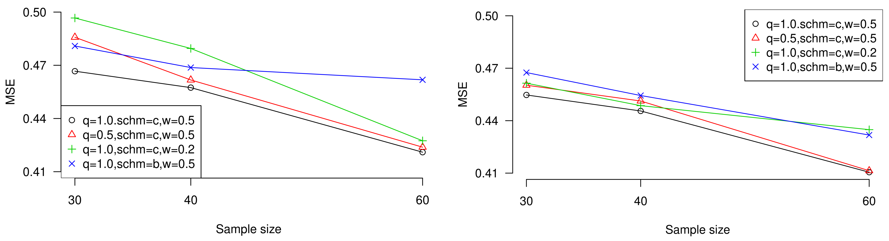
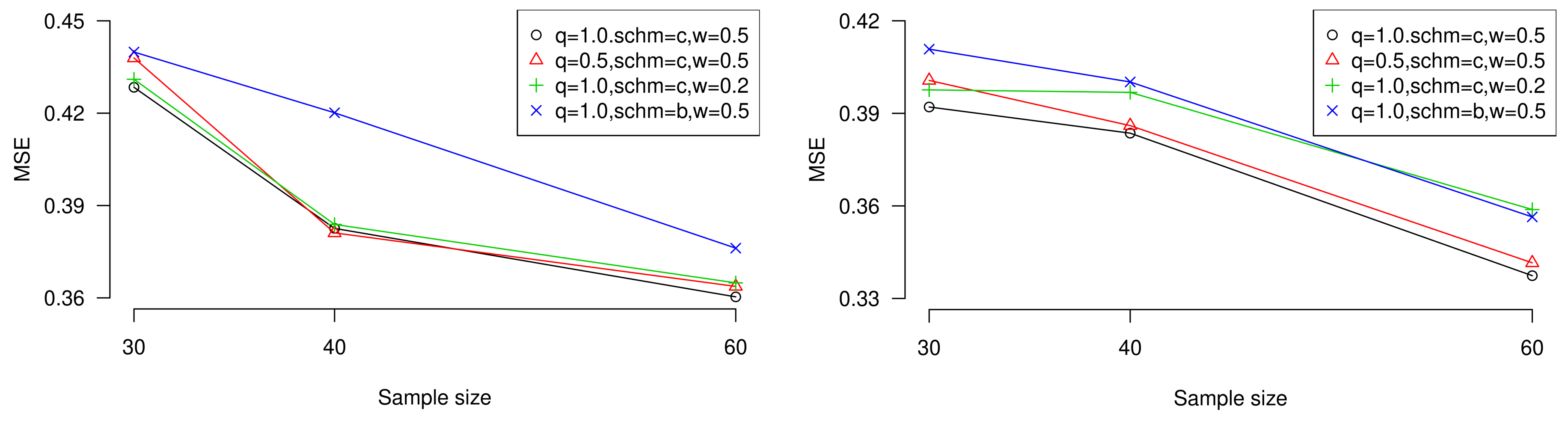
To display the conclusions, we plot the performances of MSE when sample size is increasing with different censored sizes, censoring schemes, weight of errors, and proximity of estimation towards target estimator or unknown parameter. Besides, the influence of expected experiment time T can also be observed in the figures. Trends are shown in Figure 3 and Figure 4 (values come from Table 3, Table 5, Table 7, and Table 9).

5. Real Data Analysis

To illustrate the estimations intuitively, we use a data set obtained through realistic experiment. The research started when people realized that guinea pigs are highly susceptible to human tuberculosis. Although guinea pigs do acquire resistance, even a few deadly tubercle bacilli will cause progressive disease and death. The initial focus of this investigation was the relation between numbers of tubercle bacilli infected individuals and survival time. Reference [27] used this data to test whether they can be regarded as samples from inverse Weibull distribution. According to the result, it is reasonable to use inverse Weibull distribution to analyze.
The listed values are the survival times (in days) of the guineas placed in the environment of 4.0 × 10⁶ bacillary units per 0.5 mL. Those 72 observations are shown as follows; 12, 15, 22, 24, 24, 32, 32, 33, 34, 38, 38, 43, 44, 48, 52, 53, 54, 54, 55, 56, 57, 58, 58, 59, 60, 60, 60, 60, 61, 62, 63, 65, 65, 67, 68, 70, 70, 72, 73, 75, 76, 76, 81, 83, 84, 85, 87, 91, 95, 96, 98, 99, 109, 110, 121, 127, 129, 131, 143, 146, 146, 175, 175, 211, 233, 258, 258, 263, 297, 341, 341, 376.
We first generate progressive type-II censoring scheme with ( R 1 , , R 18 ) = ( 4 , 4 , , 4 ) , and the sample is 15, 22, 32, 43, 48, 56, 60, 65, 68, 76, 87, 99, 121, 127, 146, 175, 233, 297.
For case I data set, we assume T = 90 , R 1 1 = R 2 1 = = R 11 1 = 4 , while R 12 1 = = R 17 1 = 0 and R 18 1 = 28 .
For case II data set, we assume T = 300 and scheme changes into R 1 2 = R 2 2 = = R 18 2 = 4 .
Some other values about the inverse Weibull distribution and the loss function must be given before estimations. Without informative prior, we choose a = b = s = t = 0 . Meanwhile, the influence of overestimation and underestimation are inexplicit, so against different loss functions, for consistency, we use the same h and q in simulation analysis, such that h = 1.5 , 0.5 , 1 , q = 1.5 , 0.5 , 1 . In addition, we still use w = 0.2 , 0.5 , 0.8 to carry out different balanced loss functions for estimations.
Table 11 presents the estimations of entropy under adaptive type-II progressive hybrid censoring schemes, considering all the conditions mentioned above. For convenience, we display the interval estimation entropy derived by maximum likelihood method in the same tabel.
According to the simulation study, we prefer the general entropy loss function-based Bayes estimation, where q = 1 and w = 0.5 to estimate the entropy of progressive type-II censored data reported by the infected tubercle bacilli, which has been tested to follow the inverse Weibull distribution.

6. Conclusions

Entropy of inverse Weibull distribution under different conditions are calculated and estimated in this paper. Adaptive type-II progressive hybrid censoring schemes are focused on, as they satisfy the experiment time limitation and can also be used to simulate different practical situations. Theoretically, maximum likelihood estimations, including point estimation as well as interval estimation, and Bayes estimations using three kinds of loss function, including squared error loss function, Linex loss function, and general entropy loss function, are given. Also, in general condition, considering the preference of the proximity of the target estimator to the unknown parameters, balanced loss function-based Bayes estimates are also computed. As these estimations are difficult to obtain by direct calculation, Lindley’s approximation method is applied to solve the problem numerically.
In expectation of clear comparison among all the estimations, we compute the interval length, MSE, as well as bias of them by simulation. From the results, some suggestions about estimation choices for inverse Weibull distribution without informative prior information under adaptive type-II progressive censoring schemes can be obtained. Finally, for illustration, a real data set, which has been proved following inverse Weibull distribution, is used for estimation application.
Macroscopically, although all the estimation errors are within a short interval, the ratio between observed failures and censored samples as well as supposed time limitation T are influential factors of estimates. The higher ratio of observed failures against censored samples, the larger T, the more accurate estimation is.
More specifically, under both MSE and bias criteria, Scheme c. is usually superior to other schemes and w = 0.5 is more suitable for balanced loss function under the noninformative prior inverse Weibull distribution. Furthermore, for noninformative inverse Weibull distribution, Bayes estimations are preferable in most conditions and general entropy estimation with parameter q = 1 is usually the most reasonable estimation.

Author Contributions

Methodology and Writing, R.X.; Supervision, W.G.

Funding

This research was supported by Project 202010004005 which was supported by National Training Program of Innovation and Entrepreneurship for Undergraduates.

Acknowledgments

The authors would like to thank the referees and the editor for their careful reading and constructive comments which led to this substantive improved version.

Conflicts of Interest

The authors declare no conflict of interest.

References

  1. Ng, H.K.T.; Kundu, D.; Chan, P.S. Statistical analysis of exponential lifetimes under an adaptive Type-II progressive censoring scheme. Nav. Res. Logist. 2010, 56, 687–698. [Google Scholar] [CrossRef]
  2. Burkschat, M.; Cramer, E.; Kamps, U. On optimal schemes in progressive censoring. Stat. Probab. Lett. 2006, 76, 1032–1036. [Google Scholar] [CrossRef]
  3. Mahmoud, M.; Soliman, A.; Ellah, A.; El-Sagheer, R. Estimation of Generalized Pareto under an Adaptive Type-II Progressive Censoring. Intell. Inf. Manag. 2013, 5, 73–83. [Google Scholar] [CrossRef]
  4. Sobhi, M.M.A.; Soliman, A.A. Estimation for the exponentiated Weibull model with adaptive Type-II progressive censored schemes. Appl. Math. Model. 2016, 40, 1180–1192. [Google Scholar] [CrossRef]
  5. Musleh, R.M.; Helu, A. Estimation of the inverse Weibull distribution based on progressively censored data: Comparative study. Reliab. Eng. Syst. Saf. 2014, 131, 216–227. [Google Scholar] [CrossRef]
  6. Singh, S.K.; Singh, U.; Kumar, D. Bayesian estimation of parameters of inverse Weibull distribution. J. Appl. Stat. 2013, 40, 1597–1607. [Google Scholar] [CrossRef]
  7. De Gusmao, F.R.; Ortega, E.M.; Cordeiro, G.M. The generalized inverse Weibull distribution. Stat. Pap. 2011, 52, 591–619. [Google Scholar] [CrossRef]
  8. Elbatal, I.; Muhammed, H.Z. Exponentiated generalized inverse Weibull distribution. Appl. Math. Sci. 2014, 8, 3997–4012. [Google Scholar] [CrossRef]
  9. Khan, M.S.; Pasha, G.R.; Pasha, A.H. Theoretical analysis of inverse weibull distribution. WSEAS Trans. Math. 2008, 7, 30–38. [Google Scholar]
  10. Erto, P. New Practical Bayes Estimators for the 2-Parameter Weibull Distribution. IEEE Trans. Reliab. 2009, 31, 194–197. [Google Scholar] [CrossRef]
  11. Sultan, K.S.; Ismail, M.A.; Al-Moisheer, A.S. Mixture of two inverse Weibull distributions: Properties and estimation. Comput. Stat. Data Anal. 2007, 51, 5377–5387. [Google Scholar] [CrossRef]
  12. Li, X.; Grace, J.R.; Bi, X.; Campbell, J.S. A new pyrolysis model based on generalized extreme value (GEV) distributions and its application to lignocellulosic biomass. Fuel 2016, 184, 211–221. [Google Scholar] [CrossRef]
  13. Elkotby, H.; Mai, V. Interference Modeling for Cellular Networks under Beamforming Transmission. IEEE Trans. Wirel. Commun. 2017, 16, 5201–5217. [Google Scholar] [CrossRef]
  14. Shannon, C.E. A Mathematical Theory of Communication; University of Illinois Press: Champaign, IL, USA, 1948. [Google Scholar]
  15. Misra, N.; Singh, H.; Demchuk, E. Estimation of the entropy of a multivariate normal distribution. J. Multivar. Anal. 2005, 92, 324–342. [Google Scholar] [CrossRef]
  16. Cho, Y.; Sun, H.; Lee, K. An Estimation of the Entropy for a Rayleigh Distribution Based on Doubly-Generalized Type-II Hybrid Censored Samples. Entropy 2014, 16, 3655–3669. [Google Scholar] [CrossRef]
  17. Cho, Y.; Sun, H.; Lee, K. Estimating the Entropy of a Weibull Distribution under Generalized Progressive Hybrid Censoring. Entropy 2015, 17, 102–122. [Google Scholar] [CrossRef]
  18. Mahmoud, M.; EL-Sagheer, R.M.; Abdallah, S. Inferences for New Weibull–Pareto Distribution Based on Progressively Type-II Censored Data. J. Stat. Appl. Probab. 2016, 5, 501–514. [Google Scholar] [CrossRef]
  19. Ahmed, E.A. Bayesian estimation based on progressive Type-II censoring from two-parameter bathtub-shaped lifetime model: An Markov chain Monte Carlo approach. J. Appl. Stat. 2014, 41, 752–768. [Google Scholar] [CrossRef]
  20. Pandey, B.N.; Omkar, R. Bayesian estimation of mean and square of mean of normal distribution using linex loss function. Commun. Stat. 2007, 21, 3369–3391. [Google Scholar] [CrossRef]
  21. Basu, A.; Ebrahimi, N. Bayesian approach to life testing and reliability estimation using asymmetric loss function. J. Stat. Plan. Inference 1992, 29, 21–31. [Google Scholar] [CrossRef]
  22. Calabria, R.; Pulcini, G. An engineering approach to Bayes estimation for the Weibull distribution. Microelectron. Reliab. 1994, 34, 789–802. [Google Scholar] [CrossRef]
  23. Hu, G.; Ping, P. All admissible linear estimators of a regression coefficient under a balanced loss function. J. Multivar. Anal. 2011, 102, 1217–1224. [Google Scholar] [CrossRef]
  24. Rodrigues, J.; Zellner, A. Weighted balanced loss function and estimation of the mean time to failure. Commun. Stat. 2007, 23, 3609–3616. [Google Scholar] [CrossRef]
  25. Singh, P.K.; Singh, S.K.; Singh, U. Bayes Estimator of Inverse Gaussian Parameters Under General Entropy Loss Function Using Lindley’s Approximation. Commun. Stat. Simul. Comput. 2008, 37, 1750–1762. [Google Scholar] [CrossRef]
  26. Preda, V.; Panaitescu, E.; Constantinescu, A. Bayes estimators of Modified-Weibull distribution parameters using Lindley’s approximation. WSEAS Trans. Math. 2010, 9, 539–549. [Google Scholar]
  27. Kundu, D.; Howlader, H. Bayesian inference and prediction of the inverse Weibull distribution for Type-II censored data. Comput. Stat. Data Anal. 2010, 54, 1547–1558. [Google Scholar] [CrossRef]
Figure 1. (I)Experiment terminates beyond T.
Symmetry 11 01463 g001
Figure 2. (II)Experiment terminates before T.
Symmetry 11 01463 g002
Figure 3. Mean squared error (MSE) of entropy estimation under censoring scheme c., in the case of T = 0.7 , when m = 10 (left) and m = 15 (right).
Symmetry 11 01463 g003
Figure 4. MSE of entropy estimation under censoring scheme c., in the case of T = 1.5 , when m = 10 (left) and m = 15 (right).
Symmetry 11 01463 g004
Table 1. Censoring schemes.
SchemesCase ICase II
a. R m = n m , R i = 0 ( i 0 ) R m = n m , R i = 0 ( i 0 )
b. R m = n j s
R j + 1 = R j + 2 = = R m 1 = 0
R 1 = R 2 = = R j = s
R m = n ( m 1 ) s
R i = s , ( i m )
c. R m = n j , R j = j
R j + 1 = R j + 2 = = R m 1 = 0
R 1 = R 2 = = R j 1 = 0
R m = n m + 1 , R j = j
R j + 1 = R j + 2 = = R m 1 = 1
R 1 = R 2 = = R j 1 = 0
Table 2. Approximate variance of entropy V ( H ^ ( f ) ) .
m = 10 m = 15
n Scheme T = 0.7 T = 1.5 n Scheme T = 0.7 T = 1.5
30a.0.15450.143130a.0.10690.0732
b.0.11450.0789 b.0.08870.0630
c.0.11390.0893 c.0.07130.0730
40a.0.16240.176640a.0.11930.0766
b.0.14910.1090 b.0.10680.0692
c.0.14150.1027 c.0.13190.0671
60a.0.17070.132260a.0.10970.1570
b.0.12560.1284 b.0.09930.0779
c.0.17050.1092 c.0.10630.0867
Table 3. MSE of entropy estimations when T = 0.7 , m = 10 .
mnSchemew H ^ H ^ S H ^ L H ^ E
h = 1.5 h = 0.5h = 1.0 q = 1.5 q = 0.5q = 1.0
1030a. 5.58345.80134.87175.15795.33474.81515.23705.5881
0.2 4.72384.71465.73144.69784.69304.97304.7081
0.5 5.43974.73805.41935.24004.72075.50305.3608
0.8 5.62534.81295.20455.49644.79685.22155.5844
b. 4.96705.03794.75794.66054.89324.72654.65934.9653
0.2 5.11314.61216.22084.95814.61056.66175.0398
0.5 4.94105.10704.65434.87334.76224.95424.8088
0.8 5.09934.78455.23914.98854.75785.29265.0510
c. 4.91274.97644.60494.65774.85294.60284.65664.9129
0.2 4.93394.84444.99534.83564.79974.59524.8837
0.5 4.98074.72394.65844.94724.71584.85814.6667
0.8 4.92504.60224.65574.89724.60184.85554.7127
1040a. 5.32875.49595.03914.93155.14245.01384.96015.3268
0.2 4.61215.11244.91554.90884.74454.93564.9091
0.5 5.49604.99665.33495.26954.93534.87824.8179
0.8 5.36084.93824.94085.26734.90554.94664.9283
b. 4.87294.93114.68654.60754.82074.66764.60784.8724
0.2 4.65645.68434.78214.64524.78454.78664.6486
0.5 4.69624.64984.88304.69714.64344.77434.6873
0.8 4.88414.66554.60694.85954.66104.89254.5961
c. 4.59804.59794.55994.62794.59734.70934.62774.5977
0.2 4.82344.60214.72974.77104.60174.73044.7950
0.5 4.80914.67184.62354.77974.66344.62354.5741
0.8 4.574904.68084.62734.59784.51284.62724.6979
1060a. 4.83745.25194.78224.72925.01384.74234.73045.1381
0.2 4.79044.66724.66074.74664.65574.65964.7659
0.5 4.90674.63904.81374.84804.63464.70804.6845
0.8 5.15944.73854.72705.10074.72755.13754.7272
b. 4.68414.70094.81364.85424.67754.76994.86734.6856
0.2 5.05964.82564.71274.91764.78474.71284.9905
0.5 5.06494.74514.81464.96124.72414.81894.6182
0.8 4.68734.76554.85554.68274.75334.85814.6844
c. 4.50984.61245.08114.64084.60964.47954.33954.3107
0.2 4.68865.05194.65524.66794.96264.35434.2744
0.5 4.61034.97574.63864.50984.94104.23834.2100
0.8 4.69594.66244.78594.68264.33074.48884.2876
Table 4. Bias of entropy estimations when T = 0.7 , m = 10 .
mnSchemew H ^ H ^ S H ^ L H ^ E
h = 1.5 h = 0.5h = 1.0 q = 1.5 q = 0.5q = 1.0
1030a. −2.1167−2.0952−2.1118−2.1206−2.0979−2.0915−2.0888−2.1280
0.2 −1.9939−2.1061−2.1014−1.9939−2.0653−2.0920−2.1280
0.5 −2.0716−2.0869−2.1011−2.0716−2.0648−2.0915−2.0869
0.8 −2.0979−2.1118−2.1206−2.0979−2.1294−2.1325−2.1240
b. −2.1113−2.1093−2.0888−2.0958−2.1109−2.1297−2.1324−2.1239
0.2 −2.0776−2.0321−2.1328−2.0776−2.0800−2.0787−2.0722
0.5 −2.0720−2.1229−2.1064−2.0720−2.0776−2.0799−2.0794
0.8 −2.1109−2.0888−2.0958−2.1109−2.0910−2.1280−2.0653
c. −2.0986−2.1153−2.1119−2.0827−2.1164−2.0764−2.1074−2.1119
0.2 −2.0968−2.1355−2.0829−2.1070−2.1196−2.0767−2.0675
0.5 −2.0987−2.0589−2.0706−2.1058−2.1041−2.0639−2.0767
0.8 −2.1164−2.1119−2.0827−2.0707−2.0280−2.0129−2.0776
1040a. −2.1051−2.1025−2.1242−2.0850−2.1046−2.0432−2.1004−2.0772
0.2 −2.1146−2.0912−2.1121−2.1146−2.1073−2.1059−2.1196
0.5 −2.1105−2.0823−2.1367−2.1075−2.1198−2.0764−2.1074
0.8 −2.1046−2.1242−2.0850−2.0982−2.0891−2.0386−2.1010
b. −2.0802−2.0766−2.0754−2.0652−2.0742−2.0680−2.0646−2.0608
0.2 −2.0624−2.0684−2.0616−2.0624−2.0642−2.0592−2.0584
0.5 −2.0613−2.0687−2.0629−2.0617−2.0615−2.0541−2.0535
0.8 −2.0642−2.0654−2.0632−2.0644−2.0607−2.0572−2.0589
c. −2.0462−2.0449−2.0503−2.0510−2.0419−2.0419−2.0412−2.0448
0.2 −2.0521−2.0392−2.0444−2.0402−2.0412−2.0318−2.0315
0.5 −2.0351−2.0335−2.0371−2.3651−2.0359−1.9737−1.9419
0.8 −2.0491−2.0432−2.0402−2.0379−2.0375−2.0278−2.0253
1060a. −2.0719−2.0663−2.0979−2.1074−2.0708−2.1057−2.0764−2.1058
0.2 −2.0609−2.1206−1.9785−2.0999−2.1014−2.1012−2.1006
0.5 −2.0741−2.0436−2.1078−2.1054−2.0807−2.0767−2.0639
0.8 −2.0708−2.0979−2.1074−2.0697−2.0852−2.1102−2.1059
b. −2.0335−2.0230−2.0876−2.0524−2.0400−2.1215−2.0822−2.0417
0.2 −2.0970−2.1007−2.0072−2.0560−2.0503−1.9847−1.9246
0.5 −2.0410−2.0969−2.0334−2.0580−2.0860−1.9478−1.8593
0.8 −2.0314−2.0876−2.0524−2.0124−1.9702−1.9698−1.9309
c. −2.0107−2.0121−2.0024−2.0051−2.0019−2.0002−2.0019−1.9412
0.2 −2.0151−2.0125−2.0009−2.0026−2.0023−2.0040−1.9215
0.5 −2.0166−2.0064−2.0017−1.9684−1.9822−1.9185−1.9141
0.8 −2.0125−2.0047−2.0048−1.9987−1.9857−1.9641−1.9371
Table 5. MSE of entropy estimations when T = 0.7 , m = 15 .
mnSchemew H ^ H ^ S H ^ L H ^ E
h = 1.5 h = 0.5h = 1.0 q = 1.5 q = 0.5q = 1.0
1530a. 5.35875.47474.70445.41515.20404.68815.53875.3588
0.2 4.80565.68985.05724.76715.50775.08764.7847
0.5 4.66185.06324.65184.65745.00334.65944.6517
0.8 5.17124.98665.49195.12934.98295.51935.1872
b. 4.81315.19884.62894.86335.04434.62454.87205.1316
0.2 4.89524.64244.68154.59514.83714.78094.7514
0.5 4.74964.80114.62034.73444.77884.71994.6752
0.8 5.14484.62395.10864.86554.62294.86734.7392
c. 4.73324.75004.82494.84424.72124.78674.85234.9332
0.2 4.61534.90424.61284.61374.85784.61304.6145
0.5 4.67964.69484.64234.67274.68494.60294.5471
0.8 4.73654.68544.84714.73064.77574.84874.7332
1540a. 4.98195.21595.08374.78105.65774.99434.78475.9775
0.2 4.72404.94944.95674.70334.88984.97544.7113
0.5 4.65404.59704.75874.64944.59704.75994.6508
0.8 6.02724.99344.78055.86404.96604.78125.9810
b. 4.87784.91555.31584.79554.83885.18654.91024.8772
0.2 4.59605.58964.59614.59595.42224.59614.5959
0.5 4.96844.66704.62974.91324.65974.62934.5439
0.8 4.88525.19054.90094.86855.14794.90394.8777
c. 4.52054.85244.72314.67324.79174.70094.67274.8202
0.2 4.49544.51784.57134.58064.56624.50334.4859
0.5 4.46024.50114.55744.55384.54854.51264.4556
0.8 4.52674.49904.57174.61384.59364.51164.5165
1560a. 4.92234.97084.64934.81444.86944.64014.82094.9208
0.2 4.68824.92465.14174.67164.86935.19144.6768
0.5 4.85094.70644.89624.81494.69474.90374.8330
0.8 4.93184.63904.81484.90914.63704.81614.9220
b. 4.60864.65194.64494.66964.66034.52034.46834.5063
0.2 4.67334.68774.69284.61944.55704.59224.4961
0.5 4.61714.60384.62144.61724.61794.52094.3178
0.8 4.62574.61854.66734.69674.61244.56704.4081
c. 4.35314.36244.38454.36134.34984.27044.26384.2531
0.2 4.30064.31494.34394.36074.23704.26654.3486
0.5 4.35594.31394.27224.15054.20674.11394.1052
0.8 4.35494.31714.36884.35244.32564.26164.2531
Table 6. Bias of entropy estimations when T = 0.7 , m = 15 .
mnSchemew H ^ H ^ S H ^ L H ^ E
h = 1.5 h = 0.5h = 1.0 q = 1.5 q = 0.5q = 1.0
1530a. −2.0884−2.0856−2.0929−2.1351−2.0878−2.0592−2.1075−2.0672
0.2 −2.1192−2.1018−2.0814−2.1336−2.0807−2.1269−2.1336
0.5 −2.0919−2.1082−2.0750−2.1114−1.9852−2.1111−2.1127
0.8 −2.0878−2.0929−2.1351−2.0531−2.0611−2.1157−2.0600
b. −2.0700−2.0657−2.1016−2.0973−2.1336−2.0792−2.1270−2.1336
0.2 −2.0977−2.0794−2.1055−1.9974−2.1111−2.1124−2.0877
0.5 −2.0958−2.0992−2.0902−2.0656−2.1157−2.0557−2.0436
0.8 −2.0692−2.1016−2.0973−2.0807−2.1269−2.1336−2.0629
c. −2.0517−2.0452−2.0625−2.1173−2.0549−2.0847−2.0488−2.0580
0.2 −2.0629−2.0348−2.0976−2.0682−2.1037−2.0981−2.1066
0.5 −2.0963−2.0548−2.0489−2.0478−2.0560−2.1108−2.0584
0.8 −2.0504−2.0625−2.1173−2.1336−2.1336−2.0792−2.1270
1540a. −2.0596−2.0552−2.1161−2.0802−2.0567−2.1193−2.0832−2.0785
0.2 −2.1322−2.1121−2.1024−2.1019−2.1001−2.0266−2.1290
0.5 −2.0936−2.0895−2.1167−2.1021−2.0309−2.0664−2.0647
0.8 −2.0587−2.1161−2.0802−2.0548−2.1181−2.1290−2.1019
b. −2.0455−2.0391−2.1031−2.0355−2.0442−2.0605−2.0898−2.0752
0.2 −2.0870−2.0353−2.0594−2.0870−2.1028−2.0506−2.0626
0.5 −2.1071−2.0681−2.1086−2.1041−2.0785−2.0371−2.0343
0.8 −2.0442−2.1031−2.0355−2.0442−2.1029−2.0998−2.1121
c. −2.0019−2.0093−2.0052−1.9820−1.9911−1.9806−1.9750−1.9835
0.2 −1.9887−1.9807−1.9893−1.9905−1.9866−1.9790−1.9721
0.5 −1.9903−1.9925−1.9907−1.9839−1.9790−1.9719−1.9674
0.8 −1.9953−1.9902−1.9820−1.9911−1.9956−1.9750−1.9735
1560a. −1.9920−1.9892−1.9415−1.8043−1.9915−1.9329−1.8928−1.8893
0.2 −1.9950−1.8212−1.9844−1.9893−1.9867−1.9286−1.8920
0.5 −1.8153−1.9736−1.9988−1.9898−1.9329−1.9128−1.8873
0.8 −1.9915−1.9415−1.8043−1.8170−1.9776−1.9985−1.8979
b. −1.8803−1.8769−1.8912−1.8802−1.8873−1.8820−1.8984−1.8977
0.2 −1.8092−1.8940−1.8902−1.8874−1.8986−1.8975−1.8800
0.5 −1.8097−1.8897−1.8917−1.8911−1.8708−1.8761−1.8727
0.8 −1.8796−1.8912−1.8852−1.8975−1.8847−1.8984−1.8977
c. −1.8664−1.8532−1.8666−1.8735−1.8121−1.8110−1.7498−1.8769
0.2 −1.8581−1.7491−1.8797−1.8622−1.8785−1.8498−1.8421
0.5 −1.8669−1.8494−1.8741−1.8524−1.8538−1.8341−1.8287
0.8 −1.8558−1.8666−1.8795−1.8602−1.8613−1.8527−1.8536
Table 7. MSE of entropy estimations when T = 1.5 , m = 10 .
mnSchemew H ^ H ^ S H ^ L H ^ E
h = 1.5 h = 0.5h = 1.0 q = 1.5 q = 0.5q = 1.0
1030a. 4.77754.81505.04854.75954.74924.95444.76334.7771
0.2 5.08144.79145.35564.92714.75335.48895.0064
0.5 4.74855.17144.79224.72645.07954.79564.7359
0.8 4.78474.95204.75874.77084.92114.75954.7774
b. 4.56144.43824.54764.49904.65144.56174.49254.4228
0.2 4.58404.44184.40944.43564.63634.40954.5381
0.5 4.47504.42934.42164.36504.44274.42374.3987
0.8 4.41464.44604.43064.43124.40984.49434.4594
c. 4.39674.39664.39654.39714.39674.39624.39684.3966
0.2 4.41294.46254.70704.60994.35174.40694.3102
0.5 4.40254.41224.38004.3774.41024.37944.2841
0.8 4.39674.39604.39684.39674.39594.39674.3967
1040a. 4.69744.71895.00374.59614.68514.91904.59634.6968
0.2 4.78834.46604.57114.94054.83484.75774.7183
0.5 4.56904.47394.50314.70514.40124.51374.4285
0.8 4.60164.91544.59614.69474.88824.59624.6973
b. 4.30234.30274.31974.31544.30294.31514.31584.3015
0.2 4.29004.33314.29874.28964.29074.22054.2058
0.5 4.33274.39954.32404.31224.28914.21474.2013
0.8 4.30244.31394.31464.30244.31294.27094.3021
c. 3.92043.93873.92053.82653.90563.81343.83233.8267
0.2 3.91403.97753.86623.81773.95323.87933.8385
0.5 3.86643.80263.72383.86533.89453.81113.8257
0.8 3.92403.81353.83383.91713.80843.83643.8294
1060a. 4.16004.11824.13434.11284.11274.10424.09314.1290
0.2 4.16374.13084.13564.13714.12794.10544.0957
0.5 4.07164.09344.09744.09254.08464.07614.0552
0.8 4.17004.09154.12174.13814.09384.09114.0798
b. 3.87203.89233.89593.85973.82543.88863.85963.8621
0.2 3.81343.81853.81533.80963.87313.84393.8289
0.5 3.80323.79213.74103.77263.76593.76473.7615
0.8 3.82193.79313.79673.80423.79463.79383.7621
c. 3.67173.69643.63843.90193.64303.62323.90223.6721
0.2 3.64803.64863.64403.64183.64023.64893.6360
0.5 3.64313.64373.64593.64283.64183.63723.6032
0.8 3.65643.65283.64953.64133.64163.63963.6378
Table 8. Bias of entropy estimations when T = 1.5 , m = 10 .
mnSchemew H ^ H ^ S H ^ L H ^ E
h = 1.5 h = 0.5h = 1.0 q = 1.5 q = 0.5q = 1.0
1030a. −2.1368−2.1367−2.1300−2.1287−2.1368−2.0969−2.1359−2.0393
0.2 −2.1196−2.1085−2.0973−2.1196−2.0969−2.1358−2.1196
0.5 −2.0873−2.1204−2.1026−2.0873−2.0581−2.0975−2.0943
0.8 −2.1368−2.1300−2.1287−2.1368−2.1410−2.1189−2.1284
b. −2.0902−2.0860−2.0753−2.0916−2.0893−2.1359−2.1360−2.0354
0.2 −2.0631−2.0919−2.0311−2.0631−2.0969−2.1359−2.0945
0.5 −2.0937−2.0619−2.0861−2.0937−2.0471−2.1056−2.0327
0.8 −2.0893−2.0753−2.0916−2.0893−2.1409−2.1184−2.0393
c. −2.0203−2.0027−2.0119−2.0275−2.0180−2.0354−2.0104−2.0138
0.2 −2.0317−2.0345−2.0264−2.0138−2.0269−2.0242−2.0050
0.5 −2.0212−2.0483−2.0124−2.0232−2.0101−2.0115−1.9743
0.8 −2.0180−2.1109−2.0275−2.0189−2.0345−2.0345−2.0117
1040a. −2.0814−2.0766−2.1012−2.1199−2.0804−2.0863−2.0950−2.1032
0.2 −2.0423−2.0545−2.1068−2.0423−2.1027−2.0874−2.0838
0.5 −2.0909−2.0909−2.0775−2.0909−2.1037−2.0780−2.0607
0.8 −2.0804−2.1012−2.1199−2.0804−2.0787−2.1128−2.1174
b. −2.0009−1.9977−1.9783−2.0297−2.0002−2.0075−1.9874−1.9907
0.2 −1.9626−1.9461−1.9741−1.9626−2.0027−1.9869−1.9626
0.5 −1.9449−1.9680−1.9607−1.9449−2.0029−1.9763−1.9869
0.8 −2.0002−1.9783−2.0297−2.0002−2.0369−2.0370−1.9792
c. −1.9413−1.9416−1.9195−1.9188−1.9414−1.9828−1.9636−1.9562
0.2 −1.9557−1.9475−1.9265−1.9557−1.9428−1.9542−1.9164
0.5 −1.9958−1.9396−1.9154−1.9358−1.9369−1.9292−1.9180
0.8 −1.9414−1.9195−1.9188−1.9414−1.9390−1.9369−1.9186
1060a. −2.0775−2.0750−2.0621−2.0437−2.0770−2.0877−2.0692−2.0750
0.2 −2.1062−2.0720−1.9312−2.1062−2.0749−2.0594−2.1165
0.5 −1.9563−2.0725−2.0186−1.9563−2.0369−2.0406−2.0378
0.8 −2.0770−2.0621−2.0437−2.0770−2.0378−2.0469−2.0396
b. −1.8803−1.9756−1.8805−1.9369−1.8793−1.8585−1.8539−1.8540
0.2 −1.8469−1.9045−1.8339−1.8469−1.9208−1.8988−1.8675
0.5 −1.9137−1.9298−1.8808−1.9137−1.9170−1.8540−1.8521
0.8 −1.8793−1.8805−1.9369−1.8793−1.8576−1.9160−1.8989
c. −1.8269−1.8159−1.8475−1.9321−1.8247−1.8989−1.8602−1.8568
0.2 −1.8439−1.8529−1.8705−1.8439−1.8322−1.8215−1.8188
0.5 −1.8668−1.8428−1.8427−1.8368−1.8176−1.8166−1.8156
0.8 −1.8247−1.8566−1.9001−1.8247−1.8568−1.8289−1.8302
Table 9. MSE of entropy estimations when T = 1.5 , m = 15 .
mnSchemew H ^ H ^ S H ^ L H ^ E
h = 1.5 h = 0.5h = 1.0 q = 1.5 q= 0.5q = 1.0
1530a. 4.60274.60404.75094.63424.61484.72534.63324.6028
0.2 4.61374.59294.60754.61144.52594.60694.5071
0.5 4.62484.60444.66584.62244.60384.58544.5473
0.8 4.60294.72464.63304.60274.71854.63294.6027
b. 4.29634.33864.37394.31394.29644.36014.31314.2872
0.2 4.31324.33474.36434.31074.31274.26334.1749
0.5 4.30914.30334.31134.30804.20264.11094.1081
0.8 4.29644.35894.31304.29634.25584.21284.1963
c. 4.09584.59574.02104.03174.10144.01674.03074.0957
0.2 4.12754.12844.17994.15374.09964.01103.9761
0.5 4.07254.02604.00714.01084.02314.00683.9206
0.8 4.09584.04624.03034.00954.10534.00413.9652
1540a. 4.48754.49984.59524.41084.48074.51374.41034.3672
0.2 5.36565.11004.47385.15435.02334.47284.3773
0.5 4.59544.43524.59924.59544.43194.59904.2954
0.8 4.48994.59514.41004.48614.59514.40984.4865
b. 4.07784.08904.33514.03194.07164.09414.03104.0773
0.2 4.10284.10234.10094.10174.09134.06384.0580
0.5 4.08164.12794.03884.05654.02494.03954.0018
0.8 4.18004.09334.33074.07944.08284.04054.0777
c. 3.99883.99573.99923.93683.97853.99873.93623.9657
0.2 3.97624.04933.97303.96434.01393.98233.9680
0.5 4.01643.90993.96064.02593.90843.86023.8358
0.8 3.99743.99833.93573.74563.96833.83553.8558
1560a. 4.12874.14534.11454.11174.02664.11244.10594.0854
0.2 4.14384.81244.29514.13514.12424.29514.0067
0.5 4.17054.09804.10884.07484.09484.10354.0023
0.8 4.13194.15244.11734.12604.11244.10204.1086
b. 3.73033.74433.76393.59673.72073.73983.59673.7308
0.2 3.66663.61173.62403.65894.03283.82043.6614
0.5 3.65653.59753.59603.65303.59733.59603.5642
0.8 3.63713.73243.59663.71953.73283.58743.6304
c. 3.63983.64553.12763.55173.63823.03403.70573.6403
0.2 3.69533.61643.59763.68333.61493.59783.5882
0.5 3.69643.59963.41273.48723.39923.41543.3738
0.8 3.64103.53513.45003.53953.50683.48493.4399
Table 10. Bias of entropy estimations when T = 1.5 , m = 15 .
mnSchemew H ^ H ^ S H ^ L H ^ E
h = 1.5 h = 0.5h = 1.0 q = 1.5 q = 0.5q = 1.0
1530a. −2.1294−2.1287−2.1081−2.1194−2.1292−1.9889−2.0558−1.9818
0.2 −2.1194−2.0978−2.1054−2.1194−2.1094−2.0892−2.0641
0.5 −2.1210−2.1242−2.1199−2.1210−2.1002−1.9818−1.9704
0.8 −2.1292−2.1081−2.1194−2.1292−2.0765−2.0438−2.0884
b. −1.9355−1.9352−1.9186−1.9139−1.9354−2.0503−2.0940−2.0754
0.2 −1.9402−1.9261−2.0958−1.9402−1.9169−1.9227−2.0444
0.5 −1.9197−1.9159−1.9217−1.9197−2.0294−2.0348−1.9332
0.8 −1.9354−1.9186−1.9139−1.9354−2.0236−2.0403−2.0131
c. −1.9242−1.9235−2.0976−1.9132−1.9240−2.0529−2.0622−1.9795
0.2 −1.9192−2.0742−1.9214−1.9192−1.9889−2.0616−2.0558
0.5 −1.9156−1.9235−1.9057−1.9156−2.0804−2.0497−2.0382
0.8 −1.9240−2.0976−1.9132−1.9240−2.0936−2.0910−2.0736
1540a. −1.9025−1.9005−1.9326−1.9206−1.9021−1.8503−1.8940−1.8754
0.2 −1.8451−1.8660−1.9035−1.8451−1.9176−1.9231−1.8397
0.5 −1.9346−1.9135−1.9263−1.9346−1.8940−1.8754−1.8547
0.8 −1.9021−1.9326−1.9206−1.9021−1.9333−1.8827−1.8693
b. −1.8941−1.8922−1.8893−1.9139−1.8937−1.8725−1.8681−1.8263
0.2 −1.9241−1.9249−1.8990−1.9241−1.8947−1.8899−1.8619
0.5 −1.8897−1.9154−1.8938−1.8897−1.8902−1.8693−1.8113
0.8 −1.8937−1.8893−1.9139−1.8937−1.8716−1.8267−1.8394
c. −1.8355−1.8353−1.8273−1.8126−1.8355−1.8794−1.8736−1.8264
0.2 −1.8498−1.8576−1.8417−1.8504−1.8566−1.8430−1.8396
0.5 −1.8422−1.8212−1.8367−1.8422−1.8327−1.8131−1.8097
0.8 −1.8355−1.8273−1.8126−1.8355−1.8236−1.8264−1.8142
1560a. −1.7963−1.7941−1.8203−1.8201−1.7959−1.8196−1.7792−1.8724
0.2 −1.8114−1.7641−1.7332−1.7128−1.7915−1.7960−1.7724
0.5 −1.7570−1.7726−1.7852−1.7570−1.7957−1.7934−1.7647
0.8 −1.7959−1.8203−1.7201−1.7959−1.8186−1.8170−1.7915
c. −1.7117−1.7104−1.7484−1.7272−1.7115−1.7495−1.7444−1.7431
0.2 −1.7012−1.7188−1.7278−1.7312−1.7460−1.7425−1.7365
0.5 −1.7279−1.7265−1.7347−1.7279−1.7265−1.7357−1.7273
0.8 −1.7115−1.7484−1.7272−1.7115−1.7484−1.7488−1.7457
c. −1.6225−1.6197−1.6343−1.6914−1.6239−1.6309−1.6344−1.6365
0.2 −1.6102−1.6300−1.6286−1.6327−1.6316−1.6357−1.6331
0.5 −1.6135−1.6284−1.6274−1.6215−1.6265−1.6357−1.6273
0.8 −1.6175−1.6329−1.6316−1.6297−1.6376−1.6350−1.6362
Table 11. Maximum likelihood estimations and Bayes estimations of entropy.
Casew H ^ H ^ S H ^ L H ^ E
h = 1 h = 0.5 h = 1 q = 1 q = 0.5 q = 1
I 9.0277 (±0.6263)18.252911.54926.79287.235510.13979.81909.6931
0.2 16.407911.34607.40977.50119.91739.65269.5523
0.5 13.640310.93338.97158.11089.58379.17819.1534
0.8 10.872710.218412.36409.94259.25019.41099.3486
II 8.1621 (±0.5510)20.029110.84755.16105.95729.99859.90569.8461
0.2 17.655710.64135.72206.20839.63129.51489.4559
0.5 14.095610.22047.05196.76719.08038.47198.4512
0.8 10.53559.479312.83148.14838.52948.97078.9254

