Type II Topp–Leone Inverted Kumaraswamy Distribution with Statistical Inference and Applications

Abstract

In this paper, we present and study a new four-parameter lifetime distribution obtained by the combination of the so-called type II Topp–Leone-G and transmuted-G families and the inverted Kumaraswamy distribution. By construction, the new distribution enjoys nice flexible properties and covers some well-known distributions which have already proven themselves in statistical applications, including some extensions of the Bur XII distribution. We first present the main functions related to the new distribution, with discussions on their shapes. In particular, we show that the related probability density function is left, right skewed, near symmetrical and reverse J shaped, with a notable difference regarding the right tailed, illustrating the flexibility of the distribution. Then, the related model is displayed, with the estimation of the parameters by the maximum likelihood method and the consideration of two practical data sets. We show that the proposed model is the best one in terms of standard model selection criteria, including Akaike information and Bayesian information criteria, and goodness of fit tests against three well-established competitors. Then, for the new model, the theoretical background on the maximum likelihood method is given, with numerical guaranties of the efficiency of the estimates obtained via a simulation study. Finally, the main mathematical properties of the new distribution are discussed, including asymptotic results, quantile function, Bowley skewness and Moors kurtosis, mixture representations for the probability density and cumulative density functions, ordinary moments, incomplete moments, probability weighted moments, stress-strength reliability and order statistics.

1. Introduction

The detailed explanation of a lifetime phenomenon often follows from a deep data analysis based on a well-chosen statistical model. Since the “universal best model” remains an Utopian idea, a lot of effort has been put into the construction of models with different features, involving the development of new probability distributions. The mathematical techniques for creating new probability distributions are numerous. A common technique is to introduce one or several additional tuning parameters to a standard probability distribution, with the aim to improve it, in the theoretical and practical sense. We refer the reader to the following families of distributions: the exponentiated-G (or exp-G) family [1], the beta-G family [2], the Marshall-Olkin-G family [3], the gamma-G family [4], the Kumaraswamy-G family [5], the type I half-logistic-G family [6], the transmuted-G family [7], the odd power Cauchy family [8], the exponentiated generalised Topp–Leone-G family [9], the type II Topp–Leone-G family [10] and the type II general inverse exponential-G family [11].

Let us now show some basics of the type II Topp–Leone-G family of distributions introduced by [10]. The corresponding cumulative distribution function (cdf) and probability density function (pdf) are, respectively, given by

$$F(x;\alpha ,\xi )=1-{\left\{1-{\left[G(x;\xi )\right]}^2\right\}}^{\alpha },x\in \mathbb{R}$$

and

$$f(x;\alpha ,\xi )=2\alpha g(x;\xi )G(x;\xi ){\left\{1-{\left[G(x;\xi )\right]}^2\right\}}^{\alpha -1},x\in \mathbb{R},$$

where $\alpha >0$, $G(x;\xi )$ denotes a baseline cdf of a continuous distribution which may depend on a parameter vector $\xi$ and $g(x;\xi )$ denotes the corresponding pdf. In addition to the special cases presented in [10], recent studies have highlighted the qualities of this family, and its ability to fit data sets by considering new baseline cdf $G(x;\xi )$. See, for instance, [12,13] with the consideration of the generalised Rayleigh and Rayleigh distributions as baselines, respectively. There was, however, an area that needed to be explored by considering other kinds of $G(x;\xi )$, which constituted the first piece of the idea of this study.

On the other side of things, with the aim to analyze lifetime data sets at their best, a new two-parameter distribution was introduced by [14]. It is called the inverted Kumaraswamy distribution. The corresponding cdf and pdf are, respectively, given by

$$G_{*}(x;a,b)={\left[1-{(1+x)}^{-a}\right]}^b,x>0$$

and

$$g_{*}(x;a,b)=ab{(1+x)}^{-a-1}{\left[1-{(1+x)}^{-a}\right]}^{b-1},x>0,$$

where $a,b>0$. This distribution, literally constructed from the inverse of a random variable following the so-called Kumaraswamy distribution minus one (see [15]), has been proven to be very rich. In particular, deep connexions exist with the so-called Lomax, inverted beta, log-logistic, inverted Weibull and generalised exponential distributions. However, a slight lack of flexibility can be seen in [14] (Figure 2): the hazard rate function seems to be limited in terms of curvatures (no J shape, no upside-down bathtub shape…). An immediate, elegant way to solve this problem is to extend it by using the simple transmuted technique proposed by [7]. Hence, the corresponding cdf and pdf are, respectively, given by

$$\begin{array}{cc}\hfill G(x;a,b,\lambda )& =G_{*}(x;a,b)\left[1+\lambda -\lambda G_{*}(x;a,b)\right]\hfill \\ \hfill & ={\left[1-{(1+x)}^{-a}\right]}^b\left\{1+\lambda -\lambda {\left[1-{(1+x)}^{-a}\right]}^b\right\}\hfill \end{array}$$

and

$$\begin{array}{cc}\hfill g(x;a,b,\lambda )& =g_{*}(x;a,b)\left[1+\lambda -2\lambda G_{*}(x;a,b)\right]\hfill \\ \hfill & =ab{(1+x)}^{-a-1}{\left[1-{(1+x)}^{-a}\right]}^{b-1}\left\{1+\lambda -2\lambda {\left[1-{(1+x)}^{-a}\right]}^b\right\},\hfill \end{array}$$

with $\lambda \in [-1,1]$. To the best of our knowledge, this remains a new three-parameter lifetime distribution in the literature. This constitutes the last piece of idea of the study.

That is, we introduce the type II Topp–Leone (transmuted) inverted Kumaraswamy (TIITLIK) distribution defined by combining the type II Topp–Leone-G family and the transmuted inverted Kumaraswamy distribution. We aim to offer a new ultra flexible four-parameter lifetime distribution, combining the qualities of these parents distributions, with a high potential of applicability. New statistical models for sophisticated data sets are the perspectives.

The plan of the paper is the following. In Section 2, we introduce the TIITLIK distribution, its main functions and some graphics illustrating the behaviour of the corresponding probability density and hazard rate functions. In Section 3, by the means of two practical data sets and the consideration of the maximum likelihood method, we show that the TIITLIK distribution fits better than well-established and modern adversary models. The details on the maximum likelihood method in the context of the TIITLIK distribution are given in Section 4, including a simulation study to show the nice numerical performances of the estimates. Section 5 presents the mathematical properties of the TIITLIK distribution, including asymptotes and critical points of the corresponding pdf and hrf, the quantile function, mixture representations, ordinary and central moments, incomplete moments, weighted probability moments, stress-strength reliability parameter and order statistics. Finally, some concluding remarks are given in Section 6.

2. TIITLIK Distribution

By adopting the notations above, the cdf of the TIITLIK distribution is given by

$$\begin{array}{cc}\hfill F(x;\alpha ,a,b,\lambda )& =1-{\left\{1-{\left[G(x;a,b,\lambda )\right]}^2\right\}}^{\alpha }\hfill \\ \hfill & =1-{\left\{1-{\left[1-{(1+x)}^{-a}\right]}^{2b}{\left\{1+\lambda -\lambda {\left[1-{(1+x)}^{-a}\right]}^b\right\}}^2\right\}}^{\alpha },x>0,\hfill \end{array}$$

(1)

with $\alpha ,a,b>0$ and $\lambda \in [-1,1]$. To illustrate the richness of this cdf, some special cases are described below. When $\alpha =1$, we get the cdf of the two exponentiated, transmuted, inverted Kumaraswamy distributions with parameters a, b and $\lambda$. When $\lambda =0$, we get the cdf of the Kumaraswamy inverted Kumaraswamy distribution with parameters $\alpha$, a and $2b$. When $\alpha =1$ and $\lambda =0$, we get the cdf of the inverted Kumaraswamy distribution with parameters a and $2b$. All these special cases contain several notable special cases themselves.

The survival function (sf) of the TIITLIK distribution is given by

$$\begin{array}{cc}\hfill R(x;\alpha ,a,b,\lambda )& =1-F(x;\alpha ,a,b,\lambda )\hfill \\ \hfill & ={\left\{1-{\left[1-{(1+x)}^{-a}\right]}^{2b}{\left\{1+\lambda -\lambda {\left[1-{(1+x)}^{-a}\right]}^b\right\}}^2\right\}}^{\alpha },x>0.\hfill \end{array}$$

Upon differentiation of $F(x;\alpha ,a,b,\lambda )$, the corresponding pdf is given by

$$\begin{array}{cc}\hfill & f(x;\alpha ,a,b,\lambda )=2\alpha g(x;a,b,\lambda )G(x;a,b,\lambda ){\left\{1-{\left[G(x;a,b,\lambda )\right]}^2\right\}}^{\alpha -1}\hfill \\ \hfill & =2\alpha ab{(1+x)}^{-a-1}{\left[1-{(1+x)}^{-a}\right]}^{2b-1}\left\{1+\lambda -2\lambda {\left[1-{(1+x)}^{-a}\right]}^b\right\}\times \hfill \\ \hfill & \left\{1+\lambda -\lambda {\left[1-{(1+x)}^{-a}\right]}^b\right\}{\left\{1-{\left[1-{(1+x)}^{-a}\right]}^{2b}{\left\{1+\lambda -\lambda {\left[1-{(1+x)}^{-a}\right]}^b\right\}}^2\right\}}^{\alpha -1},\hfill \\ \hfill & x>0.\hfill \end{array}$$

(2)

The corresponding hazard rate function (hrf) and cumulative hazard rate function (chrf) are, respectively, given by

$$\begin{array}{cc}\hfill & h(x;\alpha ,a,b,\lambda )=\frac{f(x;\alpha ,a,b,\lambda )}{R(x;\alpha ,a,b,\lambda )}\hfill \\ \hfill & =2\alpha ab{(1+x)}^{-a-1}{\left[1-{(1+x)}^{-a}\right]}^{2b-1}\left\{1+\lambda -2\lambda {\left[1-{(1+x)}^{-a}\right]}^b\right\}\times \hfill \\ \hfill & \left\{1+\lambda -\lambda {\left[1-{(1+x)}^{-a}\right]}^b\right\}{\left\{1-{\left[1-{(1+x)}^{-a}\right]}^{2b}{\left\{1+\lambda -\lambda {\left[1-{(1+x)}^{-a}\right]}^b\right\}}^2\right\}}^{-1},\hfill \\ \hfill & x>0\hfill \end{array}$$

and

$$\begin{array}{cc}\hfill & H(x;\alpha ,a,b,\lambda )=-log\left[R\right(x;\alpha ,a,b,\lambda \left)\right]\hfill \\ \hfill & =-\alpha log\left\{1-{\left[1-{(1+x)}^{-a}\right]}^{2b}\left\{1+\lambda -\lambda {\left[1-{(1+x)}^{-a}\right]}^{2b}\right\}\right\},x>0.\hfill \end{array}$$

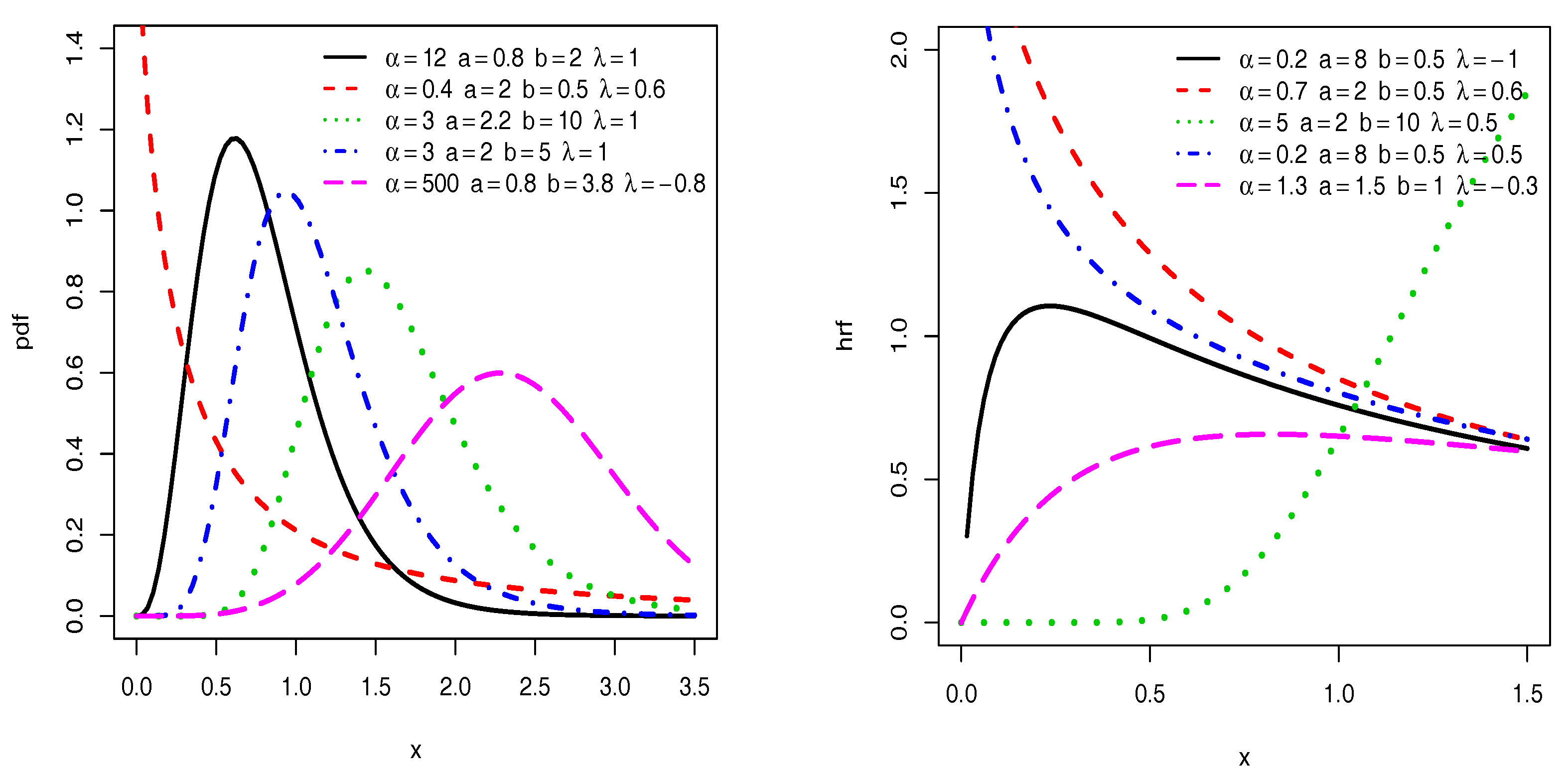
Figure 1 presents plots of the pdf and hrf of the TIITLIK distribution for fixed values of $\alpha$, a, b and $\lambda$, showing a great diversity in terms of curvature. In particular, the plots of the pdf is left, right skewed, near symmetrical and reverse J shaped, with a notable difference on the right tailed-ness. The plots of the hrf are increasing, decreasing and upside-down bathtub (contrary to the former inverted Kumaraswamy distribution; see [14] (Figure 2)). These facts ensure a great ability of the related TIITLIK model to fit a wide variety of practical data sets. This aspect will be developed in detail in Section 3.

3. Applications

We claim that the TIITLIK distribution has a high potential of applicability. In order to illustrate this claim, we analysed two practical data sets, with fair comparison to useful models in the literature, and discussions. Thus, we compared the TIHLIK distribution with the inverted Kumaraswamy (IK) distribution [14], generalised inverted Kumaraswamy (GIK) distribution by [16], Marshall–Olkin extended inverted Kumaraswamy (MOEIK) distribution [17] and Topp–Leone generalised inverted Kumaraswamy (TLGIK) distribution [18]. We refer to these papers for the exact definitions of the corresponding pdfs.

We estimated the parameters of the corresponding models by the maximum likelihood method. The estimates, called maximum likelihood estimates (MLEs), were computed using R software with the library AdequacyModel, in which the function goodness.fit was used. We refer to Section 4 for the definitions and theoretical background of the MLEs in the context of the TIITLIK model.

The following statistical measures were calculated: log-likelihood $\left(\widehat{\ell }\right)$, Akaike information criterion (AIC), Bayesian information criterion (BIC), Anderson–Darling statistic (A*) and Cramer–von Mises statistic (W*). The lower the values of these criteria, the better the fit. We also provide the value for the Kolmogorov–Smirnov (KS) statistic and its p-value.

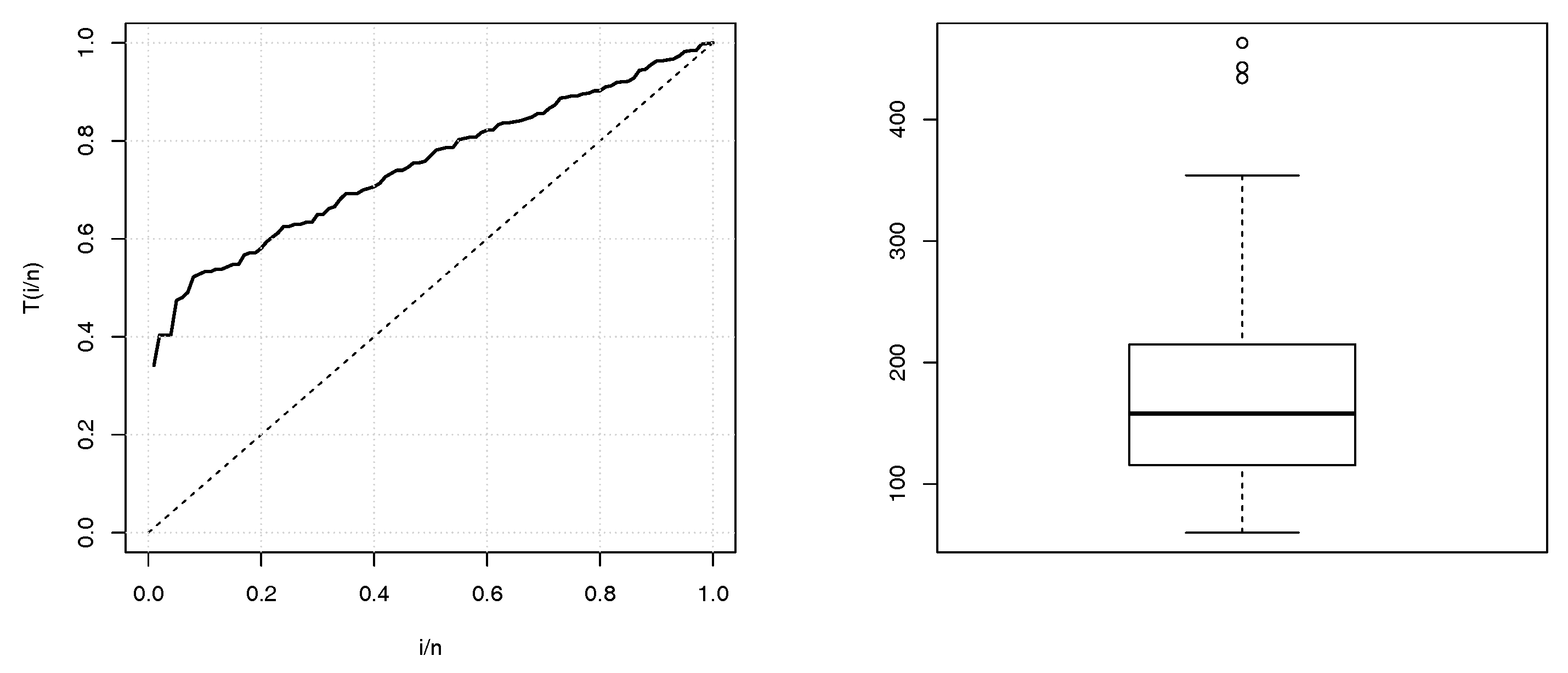
The first data set (data set 1): The first data set, given in [19], represents the annual maximum precipitation (in inches) for one rain gauge in Fort Collins (Colorado, USA) from 1900 through 1999. The heading of the data is as follows: 239, 232, 434, 85, 302, 174…

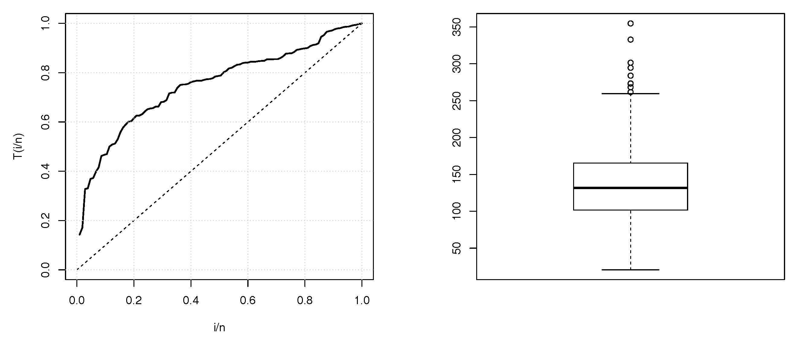
The second data set (data set 2): The second data set consists of annual maximum daily precipitation (in unit: mm) at Busan(Korea) from 1904 through 2011 period. The data set has recently been used by [20]. The heading of the data is as follows: 24.8, 140.9, 54.1, 153.5, 47.9, 165.5…

Some descriptives statistics of these two data sets are given in

Table 1. A brief statistical description of data sets 1 and 2.

	n	Mean	Median	Standard Deviation	Skewness	Kurtosis
Data set 1	100	175.67	158	83.17	1.32	1.71
Data set 2	105	144.6	131.6	66.18	0.93	0.73

. The TTT plots and boxplots for data sets 1 and 2 are shown in Figure 2 and Figure 3, respectively. From the both TTT plots, we see a concave curve, indicating that the hrf behind the data is possibly increasing. This specificity also belongs to the hrf for the TIITLIK distribution for some values, justifying its consideration for these data sets. Further detail on the TTT plots can be found in [21]. MLEs and their standard errors (in parentheses) are presented in

Table 2. Maximum likelihoods (MLEs) with their standard errors for data set 1.

Model	$\mathit{\alpha }$	a	b	$\mathit{\lambda }$	$\mathit{\beta }$	$\mathit{\theta }$
TIITLIK	6.8935	0.7683	86.5351	0.9847	-	-
	(1.0629)	(0.1939)	(2.2302)	(0.3637)	-	-
TLGIK	1.0146	-	-	1.3053	89.8279	56.2739
	(3.6755)	-	-	(4.6934)	(4.1124)	(3.8161)
MOEIK	2.5225	-	-	566.2283	576.4857	-
	(0.1234)	-	-	(25.8570)	(27.8788)	-
GIK	722.6636	-	-	-	0.5796	2.3328
	(9.2161)	-	-	-	(1.3594)	(5.4708)
IK	-	0.7465	32.1198	-	-	-
	-	(0.0409)	(6.0239)	-	-	-

and

Table 3. MLEs with their standard errors for data set 2.

Model	$\mathit{\alpha }$	a	b	$\mathit{\lambda }$	$\mathit{\beta }$	$\mathit{\theta }$
TIITLIK	35.0662	0.6705	30.7472	−0.7928	-	-
	(3.0642)	(0.1709)	(1.1182)	(0.1795)	-	-
TLGIK	1.8475	-	-	0.5927	82.5348	6.8899
	(0.5184)	-	-	(0.1581)	(7.0094)	(7.3323)
MOEIK	1.8704	-	-	99.9520	79.2607	-
	(0.0934)	-	-	(5.5420)	(6.7107)	-
GIK	351.3337	-	-	-	0.6904	1.8419
	(6.0827)	-	-	-	(3.1515)	(8.3987)
IK	-	1.1921	241.3032	-	-	-
	-	(0.0554)	(8.3953)	-	-	-

for data sets 1 and 2, respectively. The $-\widehat{\ell }$, AIC, BIC, W*, A*, KS and p-value values are provided in

Table 4. Statistical measures for data set 1.

Model	$-\widehat{\mathit{\ell }}$	AIC	BIC	W*	A*	KS	p-Value (KS)
TIITLIK	565.9951	1139.9900	1150.4110	0.0377	0.2893	0.0458	0.9847
TLGIK	567.5158	1143.0320	1153.4520	0.0644	0.4290	0.0519	0.9502
MOEIK	580.6865	1167.3730	1175.1890	0.0424	0.3156	0.1544	0.0169
GIK	593.7943	1193.5890	1201.4040	0.0472	0.3960	0.2024	0.0005
IK	644.0206	1292.0410	1297.2520	0.0410	0.3652	0.3018	0.00000002

and

Table 5. Statistical measures for data set 2.

Model	$-\widehat{\mathit{\ell }}$	AIC	BIC	W*	A*	KS	p-Value (KS)
TIITLIK	582.0684	1172.1370	1182.7530	0.1458	0.8300	0.0821	0.5000
TLGIK	600.0486	1208.0970	1218.7130	0.5001	2.8905	0.1202	0.0958
MOEIK	610.8292	1227.6580	1235.6200	0.1624	0.9319	0.2033	0.0003
GIK	616.0245	1238.0490	1246.0110	0.5327	3.0846	0.1999	0.0004
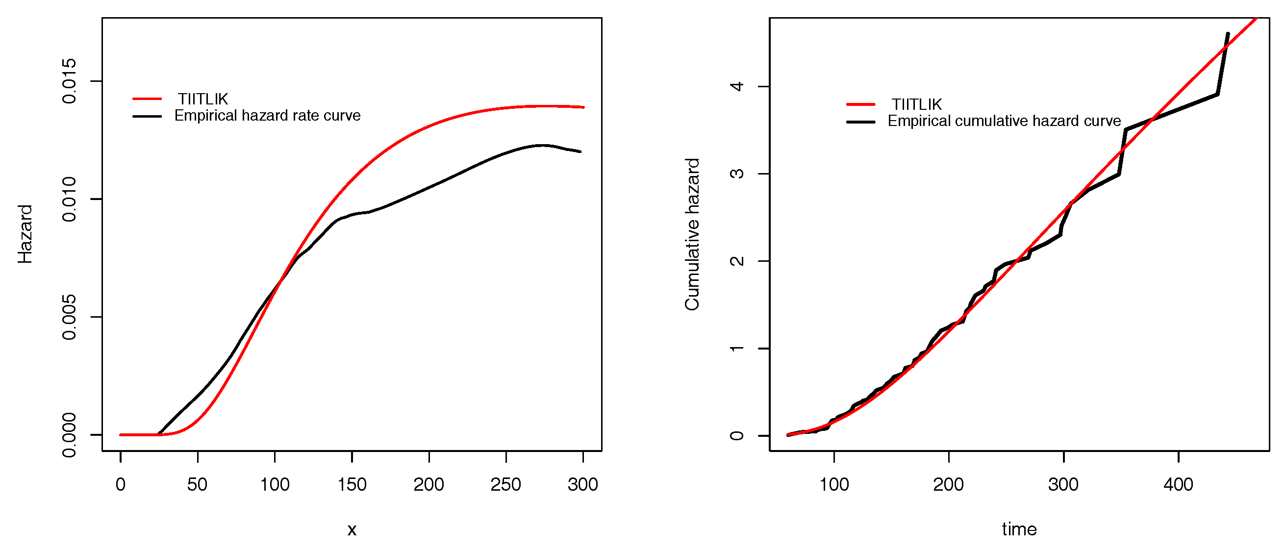
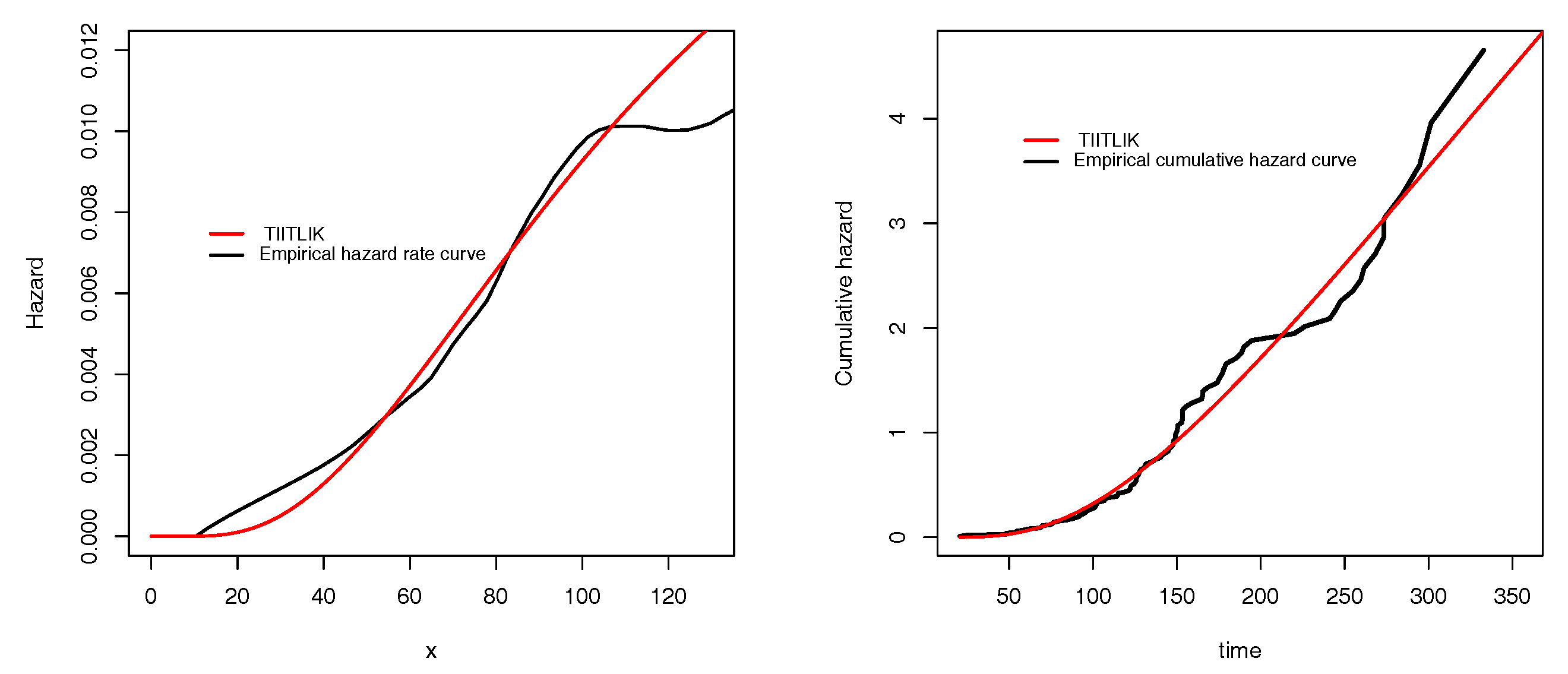
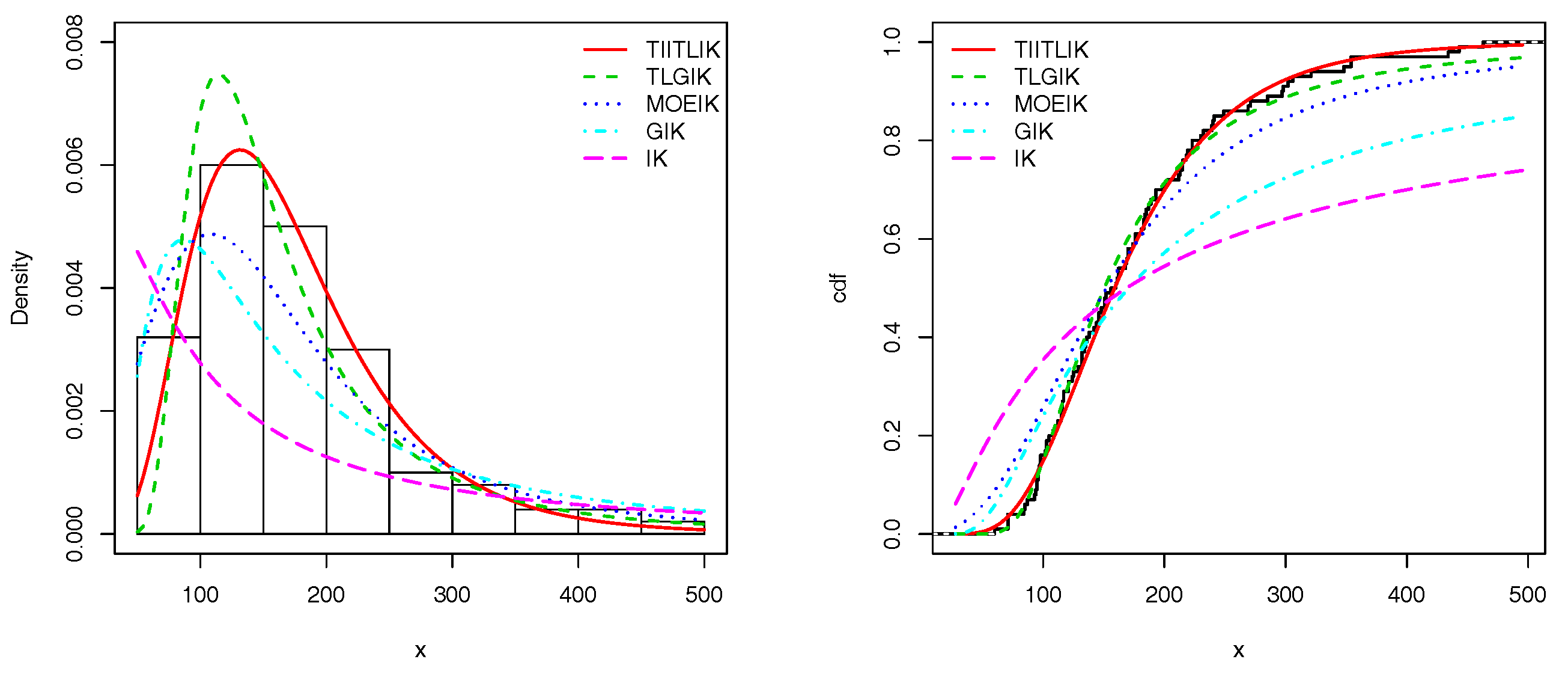
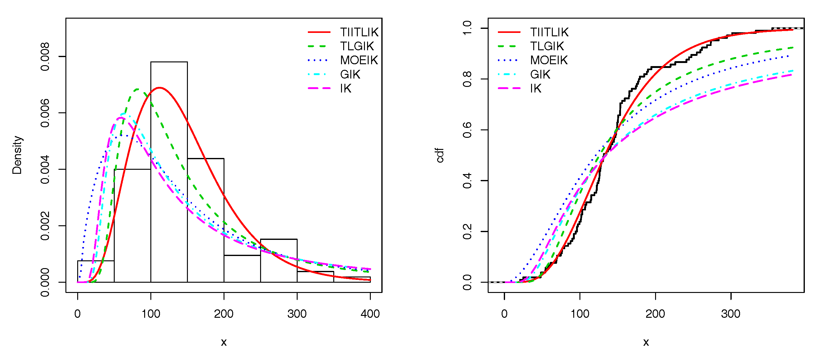
IK	620.0272	1244.0540	1249.3620	0.4794	2.7732	0.2147	0.0001

for data sets 1 and 2, respectively. In all cases, we see that the TIITLIK is the best. To illustrate this numerical fact with graphics, Figure 4 and Figure 5 present the empirical and estimated TIITLIK, hrfs and chrfs for data sets 1 and 2, respectively. Also, Figure 6 and Figure 7 show the estimated pdfs for data sets 1 and 2, respectively. For these four last figures, nice fits are observed for the TIITLIK distribution, attesting its applicability for these data sets.

4. On the MLEs of the TIITLIK Model

Here, we discuss the definitions and the convergence properties of the MLEs of the TIITLIK model used in Section 3.

4.1. Definition and Properties

Let $x_1,\dots ,x_n$ be n positive real numbers, all independent realisations of X. Then, the log-likelihood function for $\Theta =(\alpha ,a,b,\lambda )$ is given by

$$\begin{array}{cc}\hfill \ell (\Theta )& =\sum _{i=1}^{n}log\left[f(x_i;\alpha ,a,b,\lambda )\right]=nlog\left(2\right)+nlog\left(\alpha \right)+nlog\left(a\right)+nlog\left(b\right)-(a+1)\sum _{i=1}^{n}log(1+x_i)\hfill \\ \hfill & +(2b-1)\sum _{i=1}^{n}log\left[1-{(1+x_i)}^{-a}\right]+\sum _{i=1}^{n}log\left\{1+\lambda -2\lambda {\left[1-{(1+x_i)}^{-a}\right]}^b\right\}\hfill \\ \hfill & +\sum _{i=1}^{n}log\left\{1+\lambda -\lambda {\left[1-{(1+x_i)}^{-a}\right]}^b\right\}\hfill \\ \hfill & +(\alpha -1)\sum _{i=1}^{n}log\left\{1-{\left[1-{(1+x_i)}^{-a}\right]}^{2b}{\left\{1+\lambda -\lambda {\left[1-{(1+x_i)}^{-a}\right]}^b\right\}}^2\right\}.\hfill \end{array}$$

The vector of the MLEs of $\Theta$, say $\widehat{\Theta }=(\widehat{\alpha },\widehat{a},\widehat{b},\widehat{\lambda })$, are defined as the arguments of the maxima of $\ell (\Theta )$ according to $\Theta$. Thus, for the TIITLIK model, $\widehat{\alpha }$, $\widehat{a}$, $\widehat{b}$ and $\widehat{\lambda }$ can be determined as the simultaneous solutions of the following non-linear equations: $\partial \ell (\Theta )/\partial \alpha =0$, $\partial \ell (\Theta )/\partial a=0$, $\partial \ell (\Theta )/\partial b=0$ and $\partial \ell (\Theta )/\partial \lambda =0$, according to the parameters. Here, these partial derivatives can be expressed as follows:

$$\begin{array}{c}\hfill \frac{\partial \ell (\Theta )}{\partial \alpha }=\frac{n}{\alpha }+\sum _{i=1}^{n}log\left\{1-{\left[1-{(1+x_i)}^{-a}\right]}^{2b}{\left\{1+\lambda -\lambda {\left[1-{(1+x_i)}^{-a}\right]}^b\right\}}^2\right\},\end{array}$$

(3)

$$\begin{array}{cc}\hfill \frac{\partial \ell (\Theta )}{\partial a}& =\frac{n}{a}-\sum _{i=1}^{n}log(1+x_i)\hfill \\ \hfill & +(2b-1)\sum _{i=1}^n\frac{{(1+x_i)}^{-a}log(1+x_i)}{1-{(1+x_i)}^{-a}}-2b\lambda \sum _{i=1}^n\frac{{(1+x_i)}^{-a}log(1+x_i){[1-{(1+x_i)}^{-a}]}^{b-1}}{1+\lambda -2\lambda {\left[1-{(1+x_i)}^{-a}\right]}^b}\hfill \\ \hfill & -b\lambda \sum _{i=1}^n\frac{{(1+x_i)}^{-a}log(1+x_i){[1-{(1+x_i)}^{-a}]}^{b-1}}{1+\lambda -\lambda {\left[1-{(1+x_i)}^{-a}\right]}^b}\hfill \\ \hfill & +2b(\alpha -1)\sum _{i=1}^n\frac{{(1+x_i)}^{-a}log(1+x_i){\left[1-{(1+x_i)}^{-a}\right]}^{2b-1}\left\{1+\lambda -\lambda {\left[1-{(1+x_i)}^{-a}\right]}^b\right\}}{1-{\left[1-{(1+x_i)}^{-a}\right]}^{2b}{\left\{1+\lambda -\lambda {\left[1-{(1+x_i)}^{-a}\right]}^b\right\}}^2}\times \hfill \\ \hfill & \left[\lambda {\left[1-{(1+x_i)}^{-a}\right]}^b-\left\{1+\lambda -\lambda {\left[1-{(1+x_i)}^{-a}\right]}^b\right\}\right],\hfill \end{array}$$

$$\begin{array}{cc}\hfill \frac{\partial \ell (\Theta )}{\partial b}& =\frac{n}{b}+2\sum _{i=1}^{n}log\left[1-{(1+x_i)}^{-a}\right]-2\lambda \sum _{i=1}^n\frac{{\left[1-{(1+x_i)}^{-a}\right]}^{b}log[1-{(1+x_i)}^{-a}]}{1+\lambda -2\lambda {\left[1-{(1+x_i)}^{-a}\right]}^b}\hfill \\ \hfill & -\lambda \sum _{i=1}^n\frac{{\left[1-{(1+x_i)}^{-a}\right]}^{b}log[1-{(1+x_i)}^{-a}]}{1+\lambda -\lambda {\left[1-{(1+x_i)}^{-a}\right]}^b}\hfill \\ \hfill & +2(\alpha -1)\sum _{i=1}^n\frac{{\left[1-{(1+x_i)}^{-a}\right]}^{2b}log[1-{(1+x_i)}^{-a}]\left\{1+\lambda -\lambda {\left[1-{(1+x_i)}^{-a}\right]}^b\right\}}{1-{\left[1-{(1+x_i)}^{-a}\right]}^{2b}{\left\{1+\lambda -\lambda {\left[1-{(1+x_i)}^{-a}\right]}^b\right\}}^2}\times \hfill \\ \hfill & \left[\lambda {\left[1-{(1+x_i)}^{-a}\right]}^b-\left\{1+\lambda -\lambda {\left[1-{(1+x_i)}^{-a}\right]}^b\right\}\right]\hfill \end{array}$$

and

$$\begin{array}{cc}\hfill \frac{\partial \ell (\Theta )}{\partial \lambda }& =\sum _{i=1}^n\frac{1-2{\left[1-{(1+x_i)}^{-a}\right]}^b}{1+\lambda -2\lambda {\left[1-{(1+x_i)}^{-a}\right]}^b}+\sum _{i=1}^n\frac{1-{\left[1-{(1+x_i)}^{-a}\right]}^b}{1+\lambda -\lambda {\left[1-{(1+x_i)}^{-a}\right]}^b}\hfill \\ \hfill & -2(\alpha -1)\sum _{i=1}^n\frac{{\left[1-{(1+x_i)}^{-a}\right]}^{2b}\left\{1-{\left[1-{(1+x_i)}^{-a}\right]}^b\right\}\left\{1+\lambda -\lambda {\left[1-{(1+x_i)}^{-a}\right]}^b\right\}}{1-{\left[1-{(1+x_i)}^{-a}\right]}^{2b}{\left\{1+\lambda -\lambda {\left[1-{(1+x_i)}^{-a}\right]}^b\right\}}^2}.\hfill \end{array}$$

One might notice that, thanks to (3), we have the following relation between the MLEs:

$$\widehat{\alpha }={\left[-\frac{1}{n}\sum _{i=1}^{n}log\left\{1-{\left[1-{(1+x_i)}^{-\widehat{a}}\right]}^{2\widehat{b}}{\left\{1+\widehat{\lambda }-\widehat{\lambda }{\left[1-{(1+x_i)}^{-\widehat{a}}\right]}^{\widehat{b}}\right\}}^2\right\}\right]}^{-1}.$$

Clearly, we have no analytical expression for the MLEs. However, nonlinear optimisation methods, such as the quasi-Newton algorithm, can be used to have a precise numerical evaluation. Under some regularity assumptions, when n is large, the sub adjacent distribution of $\widehat{\Theta }$ is close to a multivariate normal distribution ${\mathcal{N}}_4(0_4,J{\left(\widehat{\Theta }\right)}^{-1})$, where $J\left(\widehat{\Theta }\right)={\left\{-{\partial }^2\ell (\Theta )/\partial r\partial s\right\}}_{(r,s)\in {\{\alpha ,a,b,\lambda \}}^2}{\mid }_{\Theta =\widehat{\Theta }}$, (the $4\times 4$ observed information matrix evaluated at $\widehat{\Theta }$). Here, for the sake of space, we omit its expression.

4.2. Simulation

Next, in the context of the TIITLIK model, we came up with a numerical study to study the behaviour of the MLEs and the behaviour of estimated survival and hazard rate functions defined with these estimates. We generated $N=1000$ random samples of size $n=30$, 50 and 100 from X. Five sets of the parameters were assigned. The MLEs and root mean square errors (RMSEs) of a, b, $\alpha$ and $\lambda$ were determined. Then, the estimates of sf and hrf at points $x_0$ were also evaluated. We adopted the notations: $\widehat{R}\left(x_0\right)=R(x_0,\widehat{\alpha },\widehat{a},\widehat{b},\widehat{\lambda })$ and $\widehat{h}\left(x_0\right)=h(x_0,\widehat{\alpha },\widehat{a},\widehat{b},\widehat{\lambda })$ (we remind you that $\widehat{\alpha }$, $\widehat{a}$, $\widehat{b}$ and $\widehat{\lambda }$ denote the MLEs of $\alpha$, a, b and $\lambda$, respectively). The numerical results are documented in

Table 6. MLEs, RMSEs and estimated sf and hrf of the TIITLIK distribution ($a=0.5$, $b=2$, $\alpha =2$ and $\lambda =0.5$).

	Parameters	ML	RMSE		$\widehat{\mathit{R}}\left({\mathit{x}}_0\right)$			$\widehat{\mathit{h}}\left({\mathit{x}}_0\right)$
$\mathit{n}$				${\mathit{x}}_{\mathbf{0}}=\mathbf{3}$	${\mathit{x}}_{\mathbf{0}}=\mathbf{5}$	${\mathit{x}}_{\mathbf{0}}=\mathbf{7}$	${\mathit{x}}_{\mathbf{0}}=\mathbf{3}$	${\mathit{x}}_{\mathbf{0}}=\mathbf{5}$	${\mathit{x}}_{\mathbf{0}}=\mathbf{7}$
30	a	0.800	0.550
	b	2.831	1.928
	$\alpha$	2.518	2.037	0.736	0.515	0.371	0.301	0.264	0.221
	$\lambda$	0.078	0.616
50	a	0.770	0.460
	b	2.610	1.586
	$\alpha$	2.172	1.590	0.743	0.540	0.406	0.285	0.240	0.197
	$\lambda$	0.113	0.570
100	a	0.763	0.358
	b	2.451	0.910
	$\alpha$	1.716	1.007	0.750	0.565	0.442	0.253	0.205	0.165
	$\lambda$	0.184	0.469

,

Table 7. MLEs, RMSEs, and estimated sf and hrf of the TIITLIK distribution ($a=0.5$, $b=2$, $\alpha =2$ and $\lambda =0.2$).

	Parameters	ML	RMSE		$\widehat{\mathit{R}}\left({\mathit{x}}_0\right)$			$\widehat{\mathit{h}}\left({\mathit{x}}_0\right)$
$\mathit{n}$				${\mathit{x}}_{\mathbf{0}}=\mathbf{3}$	${\mathit{x}}_{\mathbf{0}}=\mathbf{5}$	${\mathit{x}}_{\mathbf{0}}=\mathbf{7}$	${\mathit{x}}_{\mathbf{0}}=\mathbf{3}$	${\mathit{x}}_{\mathbf{0}}=\mathbf{5}$	${\mathit{x}}_{\mathbf{0}}=\mathbf{7}$
30	a	0.765	0.494
	b	3.058	2.314
	$\alpha$	2.436	2.519	0.816	0.622	0.478	0.262	0.240	0.204
	$\lambda$	0.053	0.466
50	a	0.641	0.283
	b	2.374	1.232
	$\alpha$	2.088	1.538	0.823	0.665	0.546	0.253	0.218	0.176
	$\lambda$	0.072	0.435
100	a	0.652	0.265
	b	2.325	0.872
	$\alpha$	1.867	1.165	0.824	0.671	0.558	0.240	0.196	0.158
	$\lambda$	0.071	0.390

,

Table 8. MLEs, RMSEs and estimated sf and hrf of the TIITLIK distribution ($a=0.5$, $b=2$, $\alpha =3$ and $\lambda =0.5$).

	Parameters	ML	RMSE		$\widehat{\mathit{R}}\left({\mathit{x}}_0\right)$			$\widehat{\mathit{h}}\left({\mathit{x}}_0\right)$
$\mathit{n}$				${\mathit{x}}_{\mathbf{0}}=\mathbf{3}$	${\mathit{x}}_{\mathbf{0}}=\mathbf{5}$	${\mathit{x}}_{\mathbf{0}}=\mathbf{7}$	${\mathit{x}}_{\mathbf{0}}=\mathbf{3}$	${\mathit{x}}_{\mathbf{0}}=\mathbf{5}$	${\mathit{x}}_{\mathbf{0}}=\mathbf{7}$
30	a	0.879	0.644
	b	3.113	2.796
	$\alpha$	3.104	2.303	0.591	0.324	0.190	0.423	0.372	0.309
	$\lambda$	0.266	0.930
50	a	0.855	0.519
	b	2.523	1.207
	$\alpha$	2.584	1.668	0.615	0.382	0.253	0.338	0.285	0.235
	$\lambda$	0.065	0.595
100	a	0.836	0.443
	b	2.507	1.081
	$\alpha$	2.404	1.495	0.651	0.426	0.294	0.314	0.265	0.218
	$\lambda$	0.064	0.581

,

Table 9. MLEs, RMSEs and estimated sf and hrf of the TIITLIK distribution ($a=0.5$, $b=2$, $\alpha =3$ and $\lambda =0.2$).

	Parameters	ML	RMSE		$\widehat{\mathit{R}}\left({\mathit{x}}_0\right)$			$\widehat{\mathit{h}}\left({\mathit{x}}_0\right)$
$\mathit{n}$				${\mathit{x}}_{\mathbf{0}}=\mathbf{3}$	${\mathit{x}}_{\mathbf{0}}=\mathbf{5}$	${\mathit{x}}_{\mathbf{0}}=\mathbf{7}$	${\mathit{x}}_{\mathbf{0}}=\mathbf{3}$	${\mathit{x}}_{\mathbf{0}}=\mathbf{5}$	${\mathit{x}}_{\mathbf{0}}=\mathbf{7}$
30	a	0.800	0.493
	b	2.808	1.775
	$\alpha$	2.737	1.983	0.723	0.495	0.349	0.316	0.280	0.234
	$\lambda$	0.044	0.482
50	a	0.767	0.446
	b	2.623	1.453
	$\alpha$	2.521	1.85	0.728	0.513	0.374	0.313	0.268	0.221
	$\lambda$	0.068	0.466
100	a	0.740	0.354
	b	2.353	0.966
	$\alpha$	2.320	1.496	0.738	0.541	0.410	0.283	0.236	0.194
	$\lambda$	−0.00542	0.449

and

Table 10. MLEs, RMSEs and estimated sf and hrf of the TIITLIK distribution ($a=1.2$, $b=3$, $\alpha =2$ and $\lambda =0.5$).

	Parameters	ML	RMSE		$\widehat{\mathit{R}}\left({\mathit{x}}_0\right)$			$\widehat{\mathit{h}}\left({\mathit{x}}_0\right)$
$\mathit{n}$				${\mathit{x}}_{\mathbf{0}}=\mathbf{3}$	${\mathit{x}}_{\mathbf{0}}=\mathbf{5}$	${\mathit{x}}_{\mathbf{0}}=\mathbf{7}$	${\mathit{x}}_{\mathbf{0}}=\mathbf{3}$	${\mathit{x}}_{\mathbf{0}}=\mathbf{5}$	${\mathit{x}}_{\mathbf{0}}=\mathbf{7}$
30	a	1.530	0.898
	b	4.257	2.831
	$\alpha$	2.261	1.682	0.151	0.032	0.010	0.269	0.278	0.252
	$\lambda$	0.705	0.958
50	a	1.504	0.778
	b	3.945	2.433
	$\alpha$	2.068	1.486	0.191	0.052	0.020	0.265	0.257	0.229
	$\lambda$	0.620	0.917
100	a	1.464	0.721
	b	3.633	1.794
	$\alpha$	2.057	1.204	0.229	0.073	0.031	0.262	0.252	0.223
	$\lambda$	0.481	0.439

. Table 6 considers the set of parameters: ($a=0.5$, $b=2$, $\alpha =2$ and $\lambda =0.5$); Table 7 considers: ($a=0.5$, $b=2$, $\alpha =2$ and $\lambda =0.2$); Table 8 considers: ($a=0.5$, $b=2$, $\alpha =3$ and $\lambda =0.5$); Table 9 considers: ($a=0.5$, $b=2$, $\alpha =3$ and $\lambda =0.2$); and finally, Table 9 considers: ($a=1.2$, $b=3$, $\alpha =2$ and $\lambda =0.5$).

From these numerical results, we observe that the RMSEs decrease as n increases in all situations. The estimated sfs decrease when $x_0$ increases in all situations. The estimated hrfs decrease when $x_0$ increases in all situations. The estimated sfs increase as n increases in all situations. The estimated hrfs decrease as n increases in all situations.

5. Mathematical Properties

After the practical aspect, this section is devoted to the main mathematical properties of the TIITLIK distribution. Hereafter, we consider a random variable X following the TIITLIK distribution; i.e., having the cdf given by (1) and the pdf given by (2).

5.1. Asymptotic Results and Critical Points

Some asymptotic results and critical points of the main functions of the TIITLIK distribution are presented below. When $x\to 0$, by using standard equivalence formulas, we get

$$F(x;\alpha ,a,b,\lambda )\sim \alpha {(1+\lambda )}^2{a}^{2b}{x}^{2b},f(x;\alpha ,a,b,\lambda )\sim 2b\alpha {(1+\lambda )}^2{a}^{2b}{x}^{2b-1}$$

and

$$h(x;\alpha ,a,b,\lambda )\sim 2b\alpha {(1+\lambda )}^2{a}^{2b}{x}^{2b-1}.$$

Hence, the limits of these functions mainly depend on b. When $b\in (0,1/2)$, we get $f(x;\alpha ,a,b,\lambda )\to +\infty$; when $b=1/2$, we obtain $f(x;\alpha ,a,b,\lambda )\to \alpha {(1+\lambda )}^{2}a$; and when $b>1/2$, we get $f(x;\alpha ,a,b,\lambda )\to 0$. Similarly, when $b\in (0,1/2)$, we get $h(x;\alpha ,a,b,\lambda )\to +\infty$; when $b=1/2$, we obtain $h(x;\alpha ,a,b,\lambda )\to \alpha {(1+\lambda )}^{2}a$; and when $b>1/2$, we get $h(x;\alpha ,a,b,\lambda )\to 0$.

Now, when $x\to +\infty$, we get

$$F(x;\alpha ,a,b,\lambda )\sim 1-2^{\alpha }{b}^{\alpha }{x}^{-a\alpha },f(x;\alpha ,a,b,\lambda )\sim 2^{\alpha }{b}^{\alpha }a\alpha x^{-a\alpha -1}$$

and

$$h(x;\alpha ,a,b,\lambda )\sim a\alpha x^{-1}.$$

Hence, in all cases, we have $f(x;\alpha ,a,b,\lambda )\to 0$ and $h(x;\alpha ,a,b,\lambda )\to 0$. We would like to mention that $\lambda$ plays no role for these asymptotes.

Let us now study the critical points of $f(x;\alpha ,a,b,\lambda )$ and $h(x;\alpha ,a,b,\lambda )$. The critical point(s) of $f(x;\alpha ,a,b,\lambda )$ is(are) given by the solution(s) of the following equation: ${\left\{log\left[f\right(x;\alpha ,a,b,\lambda \left)\right]\right\}}^{\prime }=0$ (the derivative is according to x), where

$$\begin{array}{cc}\hfill & log\left[f(x;\alpha ,a,b,\lambda )\right]=log\left(2\right)+log\left(\alpha \right)+log\left(a\right)+log\left(b\right)-(a+1)log(1+x)\hfill \\ \hfill & +(2b-1)log\left[1-{(1+x)}^{-a}\right]+log\left\{1+\lambda -2\lambda {\left[1-{(1+x)}^{-a}\right]}^b\right\}\hfill \\ \hfill & +log\left\{1+\lambda -\lambda {\left[1-{(1+x)}^{-a}\right]}^b\right\}\hfill \\ \hfill & +(\alpha -1)log\left\{1-{\left[1-{(1+x)}^{-a}\right]}^{2b}{\left\{1+\lambda -\lambda {\left[1-{(1+x)}^{-a}\right]}^b\right\}}^2\right\}.\hfill \end{array}$$

Then, a critical point $x_0$ of $f(x;\alpha ,a,b,\lambda )$ satisfies the following equation:

$$\begin{array}{cc}\hfill & -(a+1)\frac{1}{1+x_0}+a(2b-1)\frac{{(1+x_0)}^{-a-1}}{1-{(1+x_0)}^{-a}}-2ab\lambda \frac{{(1+x_0)}^{-a-1}{\left[1-{(1+x_0)}^{-a}\right]}^{b-1}}{1+\lambda -2\lambda {\left[1-{(1+x_0)}^{-a}\right]}^b}+\hfill \\ \hfill & -ab\lambda \frac{{(1+x_0)}^{-a-1}{\left[1-{(1+x_0)}^{-a}\right]}^{b-1}}{1+\lambda -\lambda {\left[1-{(1+x_0)}^{-a}\right]}^b}\hfill \\ \hfill & +2(\alpha -1)ab\frac{{(1+x_0)}^{-a-1}{\left[1-{(1+x_0)}^{-a}\right]}^{2b-1}\left\{1+\lambda -\lambda {\left[1-{(1+x_0)}^{-a}\right]}^b\right\}}{1-{\left[1-{(1+x_0)}^{-a}\right]}^{2b}{\left\{1+\lambda -\lambda {\left[1-{(1+x_0)}^{-a}\right]}^b\right\}}^2}\times \hfill \\ \hfill & \left[\lambda {\left[1-{(1+x_0)}^{-a}\right]}^b-\left\{1+\lambda -\lambda {\left[1-{(1+x_0)}^{-a}\right]}^b\right\}\right]=0.\hfill \end{array}$$

The nature of $x_0$ can be determined by investigating the sign of ${\left\{log\left[f\right(x;\alpha ,a,b,\lambda \left)\right]\right\}}^{″}{\mid }_{x=x_0}$. Due to the complexity of these equations, for given values of $\alpha$, a, b and $\lambda$, one can make use of mathematical software to determine $x_0$: R, Mathematica, Matlab, etc.

Similarly, the critical point(s) of $h(x;\alpha ,a,b,\lambda )$ is(are) given by the solution(s) of the following equation: ${\left\{log\left[h\right(x;\alpha ,a,b,\lambda \left)\right]\right\}}^{\prime }=0$. If such a critical point is denoted by $x_{*}$, it satisfies the following equation:

$$\begin{array}{cc}\hfill & -(a+1)\frac{1}{1+x_{*}}+a(2b-1)\frac{{(1+x_{*})}^{-a-1}}{1-{(1+x_{*})}^{-a}}-2ab\lambda \frac{{(1+x_{*})}^{-a-1}{\left[1-{(1+x_{*})}^{-a}\right]}^{b-1}}{1+\lambda -2\lambda {\left[1-{(1+x_{*})}^{-a}\right]}^b}+\hfill \\ \hfill & -ab\lambda \frac{{(1+x_{*})}^{-a-1}{\left[1-{(1+x_{*})}^{-a}\right]}^{b-1}}{1+\lambda -\lambda {\left[1-{(1+x_{*})}^{-a}\right]}^b}\hfill \\ \hfill & -2ab\frac{{(1+x_{*})}^{-a-1}{\left[1-{(1+x_{*})}^{-a}\right]}^{2b-1}\left\{1+\lambda -\lambda {\left[1-{(1+x_{*})}^{-a}\right]}^b\right\}}{1-{\left[1-{(1+x_{*})}^{-a}\right]}^{2b}{\left\{1+\lambda -\lambda {\left[1-{(1+x_{*})}^{-a}\right]}^b\right\}}^2}\times \hfill \\ \hfill & \left[\lambda {\left[1-{(1+x_{*})}^{-a}\right]}^b-\left\{1+\lambda -\lambda {\left[1-{(1+x_{*})}^{-a}\right]}^b\right\}\right]=0.\hfill \end{array}$$

Again, the nature of $x_{*}$ can be determined by investigating the sign of ${\left\{log\left[h\right(x;\alpha ,a,b,\lambda \left)\right]\right\}}^{″}{\mid }_{x=x_{*}}$.

5.2. Quantile Function

The quantile function (qf) of X, say $Q(y;\alpha ,a,b,\lambda )$, is characterised by the following equation: $Q\left(F\right(y;\alpha ,a,b,\lambda );\alpha ,a,b,\lambda )=F\left(Q\right(y;\alpha ,a,b,\lambda );\alpha ,a,b,\lambda )=y$, $y\in (0,1)$. After some algebra, we obtain

$$\begin{array}{c}\hfill Q(y;\alpha ,a,b,\lambda )={\left\{1-{\left[\frac{1+\lambda -\sqrt{1+2\left[1-2\sqrt{1-{(1-y)}^{1/\alpha }}\right]\lambda +{\lambda }^2}}{2\lambda }\right]}^{1/b}\right\}}^{-1/a}-1,y\in (0,1).\end{array}$$

Several quantities can be defined via the quantile function. For instance, the second quartile (median) is given by $M=Q(1/2;\alpha ,a,b,\lambda )$ and the inter-quantile range can be expressed as $IQR=Q(3/4;\alpha ,a,b,\lambda )-Q(1/4;\alpha ,a,b,\lambda )$.

Also, one can generate values from X by using the following result. Let $x_U=Q(U;\alpha ,a,b,\lambda )$, where U denotes a random variable following the uniform distribution $\mathcal{U}(0,1)$. Then, $x_U$ follows the TIITLIK distribution. This result was used in Section 4.2.

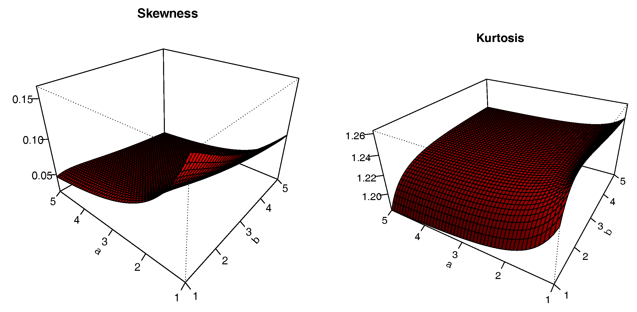
5.3. Bowley Skewness and Moors Kurtosis

The Bowley skewness and Moors kurtosis of X are defined by, respectively,

$$S=\frac{Q(6/8;\alpha ,a,b,\lambda )+Q(2/8;\alpha ,a,b,\lambda )-2Q(4/8;\alpha ,a,b,\lambda )}{IQR}$$

and

$$K=\frac{Q(7/8;\alpha ,a,b,\lambda )-Q(5/8;\alpha ,a,b,\lambda )+Q(3/8;\alpha ,a,b,\lambda )-Q(1/8;\alpha ,a,b,\lambda )}{IQR}.$$

Here, S is a measure of the asymmetry of the TIITLIK distribution and K is a measure of whether the TIITLIK distributions are heavy-tailed or light-tailed (relatively to a normal distribution). These measures have the advantage of always being well-defined from the mathematical point of view, contrary to other skewness and kurtosis measures (based on moments, for instance). More detail can be found in [22] for the Bowley skewness and [23] for the Moors kurtosis.

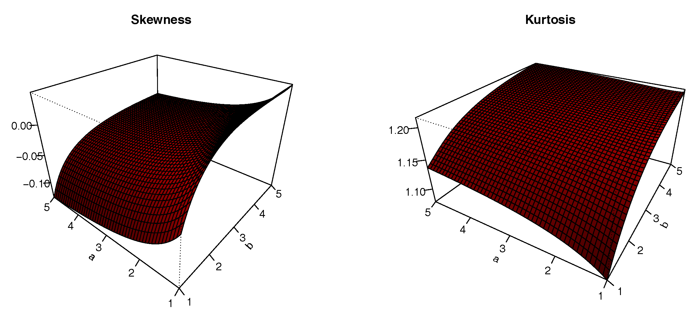
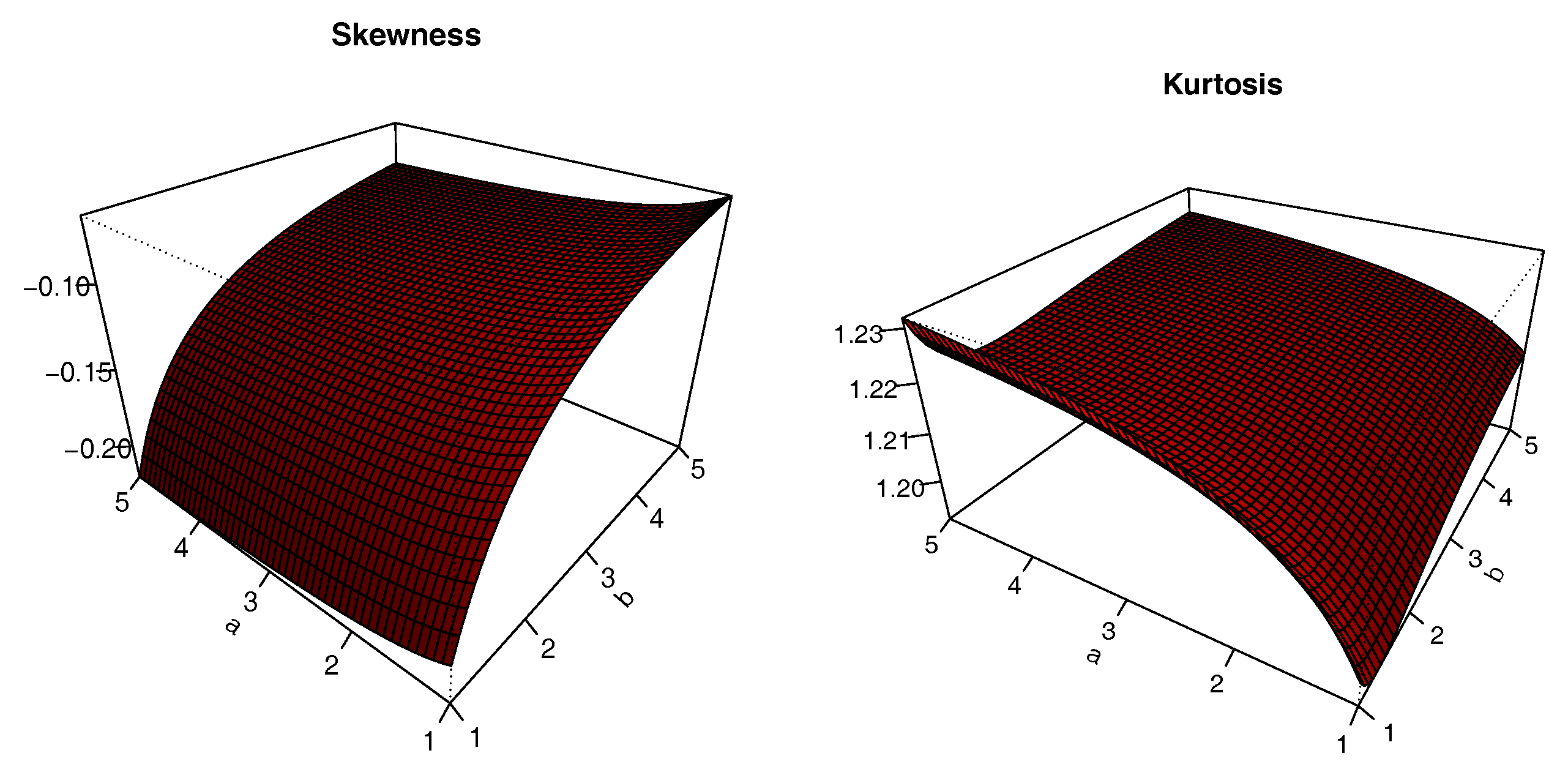
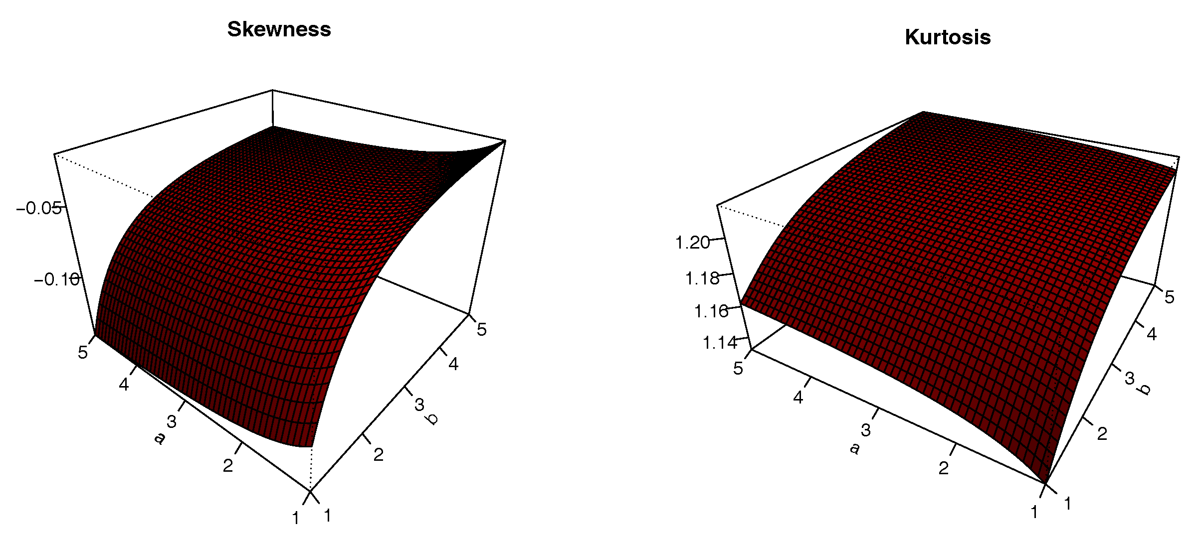
The plots of S and K are presented in Figure 8, Figure 9, Figure 10 and Figure 11 for $\alpha ,a\in (1,5)$, $b=5$ and varying values for $\lambda$; i.e., $\lambda \in \{-0.3,-0.8,0.3,0.8\}$. The impacts of the values of the parameters on S and K are significant; we can see that S can be both positive and negative, with complex variations. Similarly, K either increases or decreases, depending on the values of the parameters.

5.4. Mixture Representations

The three following results present a mixture of representations of some functions of the TIITLIK distribution in terms of Lomax distribution functions. In the proofs, for the sake of simplicity, we adopted the notation introduced in Section 1.

Proposition 1.

The following is a mixture representation for $F(x;\alpha ,a,b,\lambda )$:

$$\begin{array}{c}\hfill F(x;\alpha ,a,b,\lambda )=1-\sum _{k=0}^{+\infty }\sum _{\ell =0}^{2k}\sum _{m=0}^{+\infty }{\phi }_{k,\ell ,m}{S}_m(x;a),\end{array}$$

where ${\phi }_{k,\ell ,m}=\left(\genfrac{}{}{0pt}{}{\alpha }{k}\right)\left(\genfrac{}{}{0pt}{}{2k}{\ell }\right)\left(\genfrac{}{}{0pt}{}{b(\ell +2k)}{m}\right){(-1)}^{k+\ell +m}{(1+\lambda )}^{2k-\ell }{\lambda }^{\ell }$, (with $\left(\genfrac{}{}{0pt}{}{v}{u}\right)=v(v-1)\dots (v-u+1)/u!$) and $S_m(x;a)$ denote the sf of the Lomax distribution with parameters $am$ and 1; i.e., $S_m\left(x\right)={(1+x)}^{-am}$.

Proof. 

Since $G(x;a,b,\lambda )\in (0,1)$ (excluding the limit points), the generalised binomial formula gives

$$\begin{array}{cc}\hfill F(x;\alpha ,a,b,\lambda )& =1-\sum _{k=0}^{+\infty }\left(\genfrac{}{}{0pt}{}{\alpha }{k}\right){(-1)}^k{\left[G(x;a,b,\lambda )\right]}^{2k}.\hfill \end{array}$$

Furthermore, it follows from the standard binomial formula that

$$\begin{array}{cc}\hfill {\left[G(x;a,b,\lambda )\right]}^{2k}& ={\left[G_{*}(x;a,b)\right]}^{2k}{\left[1+\lambda -\lambda G_{*}(x;a,b)\right]}^{2k}\hfill \\ \hfill & =\sum _{\ell =0}^{2k}\left(\genfrac{}{}{0pt}{}{2k}{\ell }\right){(1+\lambda )}^{2k-\ell }{(-\lambda )}^{\ell }{\left[G_{*}(x;a,b)\right]}^{\ell +2k}.\hfill \end{array}$$

Since ${(1+x)}^{-a}\in (0,1)$, by applying again the generalised binomial formula, we have

$${\left[G_{*}(x;a,b)\right]}^{\ell +2k}={\left[1-{(1+x)}^{-a}\right]}^{b(\ell +2k)}=\sum _{m=0}^{+\infty }\left(\genfrac{}{}{0pt}{}{b(\ell +2k)}{m}\right){(-1)}^m{S}_m(x;a).$$

We end the proof by combining the above equalities together. □

Proposition 2.

We have the following mixture representation for $f(x;\alpha ,a,b,\lambda )$:

$$\begin{array}{c}\hfill f(x;\alpha ,a,b,\lambda )=\sum _{k=0}^{+\infty }\sum _{\ell =0}^{2k}\sum _{m=1}^{+\infty }{\phi }_{k,\ell ,m}{f}_m(x;a),\end{array}$$

where ${\phi }_{k,\ell ,m}$ is defined as in Proposition 1 and $f_m(x;a)$ denotes the pdf of the Lomax distribution with parameters $am$ and 1, i.e., $f_m(x;a)=am{(1+x)}^{-am-1}$.

Proof. 

The result follows from differentiation of the mixture expansion of $F(x;\alpha ,a,b,\lambda )$ established in Proposition 1. □

Owing to Proposition 2, we can exploit the properties of the Lomax distribution to derive new properties for the TIITLIK distribution. This methodology will be used in the next subsections.

Proposition 3.

Let ξ be a positive integer. Then, we have the following mixture representation:

$$\begin{array}{c}\hfill f(x;\alpha ,a,b,\lambda )F{(x;\alpha ,a,b,\lambda )}^{\xi }=\sum _{k=0}^{\xi +1}\sum _{\ell =0}^{+\infty }\sum _{m=0}^{2\ell }\sum _{q=1}^{+\infty }{\varphi }_{k,\ell ,m,q}^{\left(\xi \right)}{f}_q(x;a),\end{array}$$

where ${\varphi }_{k,\ell ,m,q}^{\left(\xi \right)}=\left(\genfrac{}{}{0pt}{}{\xi +1}{k}\right)\left(\genfrac{}{}{0pt}{}{\alpha k}{\ell }\right)\left(\genfrac{}{}{0pt}{}{2\ell }{m}\right)\left(\genfrac{}{}{0pt}{}{b(m+2k)}{q}\right){(-1)}^{k+\ell +m+q+1}{(\xi +1)}^{-1}{(1+\lambda )}^{2\ell -m}{\lambda }^m$ and $f_q(x;a)$ denotes the pdf of the Lomax distribution with parameters $aq$ and 1.

Proof. 

We will investigate a mixture representation for $F{(x;\alpha ,a,b,\lambda )}^{\xi +1}$ first, then consider the relation: ${\left[F{(x;\alpha ,a,b,\lambda )}^{\xi +1}\right]}^{\prime }=(\xi +1)f(x;\alpha ,a,b,\lambda )F{(x;\alpha ,a,b,\lambda )}^{\xi }$. Thus, it follows from the standard binomial formula that

$$\begin{array}{cc}\hfill F{(x;\alpha ,a,b,\lambda )}^{\xi +1}& ={\left\{1-{\left\{1-{\left[G(x;a,b,\lambda )\right]}^2\right\}}^{\alpha }\right\}}^{\xi +1}=\sum _{k=0}^{\xi +1}\left(\genfrac{}{}{0pt}{}{\xi +1}{k}\right){(-1)}^k{\left\{1-{\left[G(x;a,b,\lambda )\right]}^2\right\}}^{\alpha k}.\hfill \end{array}$$

Since $G(x;a,b,\lambda )\in (0,1)$, the generalised binomial formula gives

$$\begin{array}{c}\hfill {\left\{1-{\left[G(x;a,b,\lambda )\right]}^2\right\}}^{\alpha k}=\sum _{\ell =0}^{+\infty }\left(\genfrac{}{}{0pt}{}{\alpha k}{\ell }\right){(-1)}^{\ell }{\left[G(x;a,b,\lambda )\right]}^{2\ell }.\end{array}$$

Then, we should proceed as in the proof of Proposition 1. The standard binomial formula gives

$$\begin{array}{c}\hfill {\left[G(x;a,b,\lambda )\right]}^{2\ell }=\sum _{m=0}^{2\ell }\left(\genfrac{}{}{0pt}{}{2\ell }{m}\right){(1+\lambda )}^{2\ell -m}{(-\lambda )}^m{\left[G_{*}(x;a,b)\right]}^{m+2\ell }\end{array}$$

and, by the generalised binomial formula using ${(1+x)}^{-a}\in (0,1)$, we get

$$\begin{array}{c}\hfill {\left[G_{*}(x;a,b)\right]}^{m+2k}=\sum _{q=0}^{+\infty }\left(\genfrac{}{}{0pt}{}{b(m+2k)}{q}\right){(-1)}^q{S}_q(x;a).\end{array}$$

By putting the above equalities together, we get

$$F{(x;\alpha ,a,b,\lambda )}^{\xi +1}=\sum _{k=0}^{\xi +1}\sum _{\ell =0}^{+\infty }\sum _{m=0}^{2\ell }\sum _{q=0}^{+\infty }{\psi }_{k,\ell ,m,q}^{\left(\xi \right)}{S}_q(x;a),$$

where ${\psi }_{k,\ell ,m,q}^{\left(\xi \right)}=\left(\genfrac{}{}{0pt}{}{\xi +1}{k}\right)\left(\genfrac{}{}{0pt}{}{\alpha k}{\ell }\right)\left(\genfrac{}{}{0pt}{}{2\ell }{m}\right)\left(\genfrac{}{}{0pt}{}{b(m+2k)}{q}\right){(-1)}^{k+\ell +m+q}{(1+\lambda )}^{2\ell -m}{\lambda }^m$. Upon differentiation of this series expansion, we get

$$f(x;\alpha ,a,b,\lambda )F{(x;\alpha ,a,b,\lambda )}^{\xi }=\sum _{k=0}^{\xi +1}\sum _{\ell =0}^{+\infty }\sum _{m=0}^{2\ell }\sum _{q=1}^{+\infty }{\varphi }_{k,\ell ,m,q}^{\left(\xi \right)}{f}_q(x;a),$$

where ${\varphi }_{k,\ell ,m,q}^{\left(\xi \right)}=-{(\xi +1)}^{-1}{\psi }_{k,\ell ,m,q}^{\left(\xi \right)}$, which is the desired result. □

5.5. The Ordinary and Central Moments

Let r be a positive integer. Then, the r-th moment of X, i.e., ${\mu }_r^{\prime }=E\left(X^r\right)$, exists if, and only if, $a\alpha >r$. Under this assumption, we have

$${\mu }_r^{\prime }={\int }_0^{+\infty }{x}^{r}f(x;\alpha ,a,b,\lambda )dx.$$

For given values of $\alpha$, a, b and $\lambda$, this integral can be evaluated by any mathematical software. Additionally, one can use Proposition 2 for a series expression, which is performed below. Let us introduce the gamma function defined by $\Gamma \left(s\right)={\int }_0^{+\infty }{t}^s{e}^{-t}dt$, $s>0$. Then, by assuming that $amin(\alpha ,1)>r$ and noticing that

$${\int }_0^{+\infty }{x}^r{f}_m(x;a)dx=am\frac{\Gamma (r+1)\Gamma (am-r)}{\Gamma (am+1)}=\frac{r!}{{\prod }_{u=1}^r(am-u)},$$

we obtain

$${\mu }_r^{\prime }=\sum _{k=0}^{+\infty }\sum _{\ell =0}^{2k}\sum _{m=1}^{+\infty }{\phi }_{k,\ell ,m}{\int }_0^{+\infty }{x}^r{f}_m(x;a)dx=\sum _{k=0}^{+\infty }\sum _{\ell =0}^{2k}\sum _{m=1}^{+\infty }{\phi }_{k,\ell ,m}\frac{r!}{{\prod }_{u=1}^r(am-u)}.$$

For practical purposes, one can consider a large integer K, says $K=50$, and the approximation:

$${\mu }_r^{\prime }\approx \sum _{k=0}^K\sum _{\ell =0}^{2k}\sum _{m=1}^K{\phi }_{k,\ell ,m}\frac{r!}{{\prod }_{u=1}^r(am-u)};$$

therefore, assuming that $amin(\alpha ,1)>2$, the mean and the variance of X are given by, respectively, $\mu ={\mu }_1^{\prime }$ and ${\sigma }^2={\mu }_2^{\prime }-{\mu }^2$.

Always under the assumption $a\alpha >r$, the r-th central moment of X, i.e., ${\mu }_r=E\left[{(X-\mu )}^r\right]$, exists. It is given by

$${\mu }_r={\int }_0^{+\infty }{(x-\mu )}^{r}f(x;\alpha ,a,b,\lambda )dx.$$

The standard binomial formula gives

$$\begin{array}{c}\hfill {\mu }_r=\sum _{k=0}^r\left(\genfrac{}{}{0pt}{}{r}{k}\right){(-1)}^k{\mu }^k{\mu }_{r-k}^{\prime }.\end{array}$$

One can notice that ${\sigma }^2={\mu }_2$. Additionally, important quantities can be derived, such as the r-th cumulant of X defined by

$${\kappa }_r={\mu }_r^{\prime }-\sum _{k=1}^{r-1}\left(\genfrac{}{}{0pt}{}{r-1}{k-1}\right){\kappa }_k{\mu }_{r-k}^{\prime },$$

with ${\kappa }_1={\mu }_1^{\prime }$, and the Pearson measures of skewness and kurtosis of X defined by ${\gamma }_1={\mu }_3/{\mu }_2^{3/2}$ and ${\beta }_2={\mu }_4/{\mu }_2^2$, respectively.

5.6. Incomplete Moments

Let $t\ge 0$ and r be positive integers. Then, the r-th incomplete moment of X, i.e., ${\mu }_r^{\prime }\left(t\right)=E\left(X^r{1}_{\{X\le t\}}\right)$ exists and is given by

$${\mu }_r^{\prime }\left(t\right)={\int }_0^t{x}^{r}f(x;\alpha ,a,b,\lambda )dx=\sum _{k=0}^{+\infty }\sum _{\ell =0}^{2k}\sum _{m=1}^{+\infty }{\phi }_{k,\ell ,m}{\int }_0^t{x}^r{f}_m(x;a)dx.$$

For given values for t, $\alpha$, a, b and $\lambda$, a numerical evaluation of the integral term is possible. Incomplete moments appear naturally in several useful quantities. For instance, the mean deviations of X about the mean and the median use ${\mu }_1^{\prime }\left(t\right)$; i.e.,

$$\begin{array}{c}\hfill {\delta }_{\mu }=E\left(\right|X-\mu \left|\right)=2\mu F(\mu ;\alpha ,a,b,\lambda )-2{\mu }_1^{\prime }\left(\mu \right),{\delta }_M=E\left(\right|X-M\left|\right)=\mu -2{\mu }_1^{\prime }\left(M\right).\end{array}$$

One can also construct Lorenz and Bonferroni curves, which find applications in economics, insurance and medicine, among others.

5.7. Weighted Probability Moments

Let r and s be two positive integers. Then, the $r,s$-th weighted probability moment for X, i.e., ${\mu }_{r,s}^{\prime }=E\left(X^{r}F{(X;\alpha ,a,b,\lambda )}^s\right)$ exists if, and only if, $a\alpha >r$. It is defined by

$${\mu }_{r,s}^{\prime }={\int }_0^{+\infty }{x}^{r}f(x;\alpha ,a,b,\lambda )F{(x;\alpha ,a,b,\lambda )}^{s}dx.$$

It follows from Proposition 3 applied with $\xi =s$ that

$${\mu }_{r,s}^{\prime }=\sum _{k=0}^{s+1}\sum _{\ell =0}^{+\infty }\sum _{m=0}^{2\ell }\sum _{q=1}^{+\infty }{\varphi }_{k,\ell ,m,q}^{\left(s\right)}{\int }_0^{+\infty }{x}^r{f}_q(x;a)dx=\sum _{k=0}^{s+1}\sum _{\ell =0}^{+\infty }\sum _{m=0}^{2\ell }\sum _{q=1}^{+\infty }{\varphi }_{k,\ell ,m,q}^{\left(s\right)}\frac{r!}{{\prod }_{u=1}^r(aq-u)}.$$

The probability weighted moments naturally appear when we deal with some natural statistics, as order statistics. Further details will be presented in Section 5.9.

5.8. Stress–Strength Reliability Parameter

Let X and Y be independent random variables having the TIITLIK distribution with the sets of parameters $({\alpha }_1,a_1,b_1,{\lambda }_1)$ and $({\alpha }_2,a_2,b_2,{\lambda }_2)$, respectively. Then, the corresponding stress-strength reliability parameter is defined by $R=P(X_2<X_1)$. We should then determine it with several sets of assumptions on the parameter. We begin with a tractable result in that regard.

Proposition 4.

Under the above setting, assume that $a_1=a_2$, $b_1=b_2$ and ${\lambda }_1={\lambda }_2$. Then, we have

$$\begin{array}{c}\hfill R=\frac{{\alpha }_2}{{\alpha }_1+{\alpha }_2}.\end{array}$$

Proof. 

By using the definitions of $F(x;{\alpha }_2,a,b,\lambda )$ and $f(x;{\alpha }_1,a,b,\lambda )$, we get

$$\begin{array}{cc}\hfill & R={\int }_0^{+\infty }F(x;{\alpha }_2,a,b,\lambda )f(x;{\alpha }_1,a,b,\lambda )dx\hfill \\ \hfill & =1-{\int }_0^{+\infty }{\left\{1-{\left[1-{(1+x)}^{-a}\right]}^{2b}{\left\{1+\lambda -\lambda {\left[1-{(1+x)}^{-a}\right]}^b\right\}}^2\right\}}^{{\alpha }_2}f(x;{\alpha }_1,a,b,\lambda )dx\hfill \\ \hfill & =1-{\int }_0^{+\infty }2{\alpha }_{1}ab{(1+x)}^{-a-1}{\left[1-{(1+x)}^{-a}\right]}^{2b-1}\left\{1+\lambda -2\lambda {\left[1-{(1+x)}^{-a}\right]}^b\right\}\times \hfill \\ \hfill & \left\{1+\lambda -\lambda {\left[1-{(1+x)}^{-a}\right]}^b\right\}{\left\{1-{\left[1-{(1+x)}^{-a}\right]}^{2b}{\left\{1+\lambda -\lambda {\left[1-{(1+x)}^{-a}\right]}^b\right\}}^2\right\}}^{{\alpha }_1+{\alpha }_2-1}dx\hfill \\ \hfill & =1-\frac{{\alpha }_1}{{\alpha }_1+{\alpha }_2}{\int }_0^{+\infty }f(x;{\alpha }_1+{\alpha }_2,a,b,\lambda )dx=\frac{{\alpha }_2}{{\alpha }_1+{\alpha }_2}.\hfill \end{array}$$

The proof of Proposition 4 is ended. □

The result below proposes a more general alternative result.

Proposition 5.

Without special assumptions on the parameters, we have

$$\begin{array}{c}\hfill R=1-\sum _{k=0}^{+\infty }\sum _{\ell =0}^{2k}\sum _{m=0}^{+\infty }\sum _{u=0}^{+\infty }\sum _{v=0}^{2u}\sum _{w=0}^{+\infty }{\phi }_{k,\ell ,m}^{\left(2\right)}{\phi }_{u,v,w}^{\left(1\right)}\frac{a_{1}w}{a_{1}w+a_{2}m},\end{array}$$

where, for $j\in \{1,2\}$, ${\phi }_{k,\ell ,m}^{\left(j\right)}=\left(\genfrac{}{}{0pt}{}{{\alpha }_j}{k}\right)\left(\genfrac{}{}{0pt}{}{2k}{\ell }\right)\left(\genfrac{}{}{0pt}{}{b_j(\ell +2k)}{m}\right){(-1)}^{k+\ell +m}{(1+{\lambda }_j)}^{2k-\ell }{\lambda }_j^{\ell }$.

Proof. 

Owing to Propositions 1 and 2, we have

$$\begin{array}{cc}\hfill & R={\int }_0^{+\infty }F(x;{\alpha }_2,a_2,b_2,{\lambda }_2)f(x;{\alpha }_1,a_1,b_1,{\lambda }_1)dx\hfill \\ \hfill & =1-\sum _{k=0}^{+\infty }\sum _{\ell =0}^{2k}\sum _{m=0}^{+\infty }{\phi }_{k,\ell ,m}^{\left(2\right)}{\int }_0^{+\infty }{S}_m(x;a_2)f(x;{\alpha }_1,a_1,b_1,{\lambda }_1)dx\hfill \\ \hfill & =1-\sum _{k=0}^{+\infty }\sum _{\ell =0}^{2k}\sum _{m=0}^{+\infty }\sum _{u=0}^{+\infty }\sum _{v=0}^{2u}\sum _{w=0}^{+\infty }{\phi }_{k,\ell ,m}^{\left(2\right)}{\phi }_{u,v,w}^{\left(1\right)}{\int }_0^{+\infty }{S}_m(x;a_2)f_w(x;a_1)dx.\hfill \end{array}$$

Then, by introducing the pdf $f_{*}(x;a_{1}w+a_{2}m,1)$ of the Lomax distribution with parameters $a_{1}w+a_{2}m$ and 1, we get

$${\int }_0^{+\infty }{S}_m(x;a_2)f_w(x;a_1)dx=\frac{a_{1}w}{a_{1}w+a_{2}m}{\int }_0^{+\infty }{f}_{*}(x;a_{1}w+a_{2}m,1)dx=\frac{a_{1}w}{a_{1}w+a_{2}m}.$$

This ends the proof of Proposition 5. □

5.9. Order Statistics

Since the former study of [24], order statistics found a place as the model of choice for various phenomena dealing with the infima or suprema of random variables. Here, we present some basics on the order statistics in the context of the TIITLIK distribution. Let $X_1,\dots ,X_n$ be n independent random having the TIITLIK distribution as the common distribution and $X_{i:n}$ be the i-th order statistic defined by the i-th random variable; i.e., $X_{1:n}\le X_{2:n}\le \dots \le X_{n:n}$ after rearranging $X_1,\dots ,X_n$ in an increasing order. Then, the pdf of $X_{i:n}$ is given by

$$\begin{array}{c}\hfill f_{i:n}(x;\alpha ,a,b,\lambda )=\frac{n!}{(i-1)!(n-i)!}\sum _{j=0}^{n-i}\left(\genfrac{}{}{0pt}{}{n-i}{j}\right){(-1)}^{j}f(x;\alpha ,a,b,\lambda )F{(x;\alpha ,a,b,\lambda )}^{j+i-1},x>0.\end{array}$$

Owing to Proposition 3 applied with $\xi =j+i-1$, we obtain the following mixture representation:

$$\begin{array}{c}\hfill f_{i:n}(x;\alpha ,a,b,\lambda )=\sum _{j=0}^{n-i}\sum _{k=0}^{j+i-1}\sum _{\ell =0}^{+\infty }\sum _{m=0}^{2\ell }\sum _{q=1}^{+\infty }{\rho }_{i,j,k,\ell ,m,n,q}{f}_q(x;a),\end{array}$$

(4)

where ${\rho }_{i,j,k,\ell ,m,n,q}=n!/\left[(i-1)!(n-i)!\right]\left(\genfrac{}{}{0pt}{}{n-i}{j}\right)\left(\genfrac{}{}{0pt}{}{j+i}{k}\right)\left(\genfrac{}{}{0pt}{}{\alpha k}{\ell }\right)\left(\genfrac{}{}{0pt}{}{2\ell }{m}\right)\left(\genfrac{}{}{0pt}{}{b(m+2k)}{q}\right){(-1)}^{j+k+\ell +m+q+1}{(j+i)}^{-1}{(1+\lambda )}^{2\ell -m}{\lambda }^m$ and $f_q(x;a)$ denotes the pdf of the Lomax distribution with parameters $aq$ and 1.

Let r be a positive integer. Then, the r-th moment of $X_{i:n}$ is given by

$${\mu }_{r,i:n}^{\prime }=\sum _{j=0}^{n-i}\sum _{k=0}^{j+i-1}\sum _{\ell =0}^{+\infty }\sum _{m=0}^{2\ell }\sum _{q=1}^{+\infty }{\rho }_{i,j,k,\ell ,m,n,q}\frac{r!}{{\prod }_{u=1}^r(aq-u)}.$$

Among others, these moments can be used to define the L moments of X. Thus, for any $s\in \{1,\dots ,n\}$, the s-th L moment of X is given by

$${\Lambda }_s=\frac{1}{s}\sum _{d=0}^{s-1}{(-1)}^d\left(\genfrac{}{}{0pt}{}{s-1}{d}\right){\mu }_{1,s-d:s}^{\prime }.$$

We refer the reader to [25,26] for further details on L moments.

6. Conclusions

In this paper, we introduced a new, four-parameter lifetime distribution called the type II Topp–Leone (transmuted) inverted Kumaraswamy (TIITLIK) distribution. Two applications on practical data sets showed that the TIITLIK distribution provides better fits than several serious competitors, validating its potential in terms of applicability. In order to complete the practical aspect, we provided the main mathematical properties of the new distribution, including asymptotic results, quantile function, Bowley skewness and Moors kurtosis, mixture representations for the probability density and cumulative density functions, ordinary moments, incomplete moments, probability weighted moments, stress-strength reliability and order statistics.

References

1. Gupta, R.D.; Kundu, D. Exponentiated exponential family: An alternative to Gamma and Weibull distributions. Biom. J. 2001, 43, 117–130. [Google Scholar] [CrossRef]
2. Eugene, N.; Lee, C.; Famoye, F. Beta-normal distribution and its applications. Commun. Stat.-Theory Methods 2002, 31, 497–512. [Google Scholar] [CrossRef]
3. Marshall, A.; Olkin, I. A new method for adding a parameter to a family of distributions with applications to the exponential and Weibull families. Biometrika 1997, 84, 641–652. [Google Scholar] [CrossRef]
4. Zografos, K.; Balakrishnan, N. On families of beta- and generalized gamma-generated distributions and associated inference. Stat. Methodol. 2009, 6, 344–362. [Google Scholar] [CrossRef]
5. Alizadeh, M.; Emadiz, M.; Doostparast, M.; Cordeiro, G.M.; Ortega, E.M.M.; Pescim, R.R. A new family of distributions: The Kumaraswamy odd log-logistic, properties and applications. Hacet. J. Math. Stat. 2015, 44, 1491–1512. [Google Scholar] [CrossRef]
6. Cordeiro, G.M.; Alizadeh, M.; Marinho, E.P.R.D. The type I half-logistic family of distributions. J. Stat. Comput. Simul. 2015, 86, 707–728. [Google Scholar] [CrossRef]
7. Shaw, W.T.; Buckley, I.R. The Alchemy of Probability Distributions: Beyond Gram-Charlier Expansions, and a Skew-kurtotic-normal Distribution from a Rank Transmutation Map. arXiv 2009, arXiv:0901.0434. [Google Scholar]
8. Alizadeh, M.; Altun, E.; Cordeiro, G.M.; Rasekhi, M. The odd power Cauchy family of distributions: Properties, regression models and applications. J. Stat. Comput. Simul. 2018, 88, 785–805. [Google Scholar] [CrossRef]
9. Reyad, H.M.; Alizadeh, M.; Jamal, F.; Othman, S.; Hamedani, G.G. The Exponentiated Generalized Topp-Leone-G Family of Distributions: Properties and Applications. Pak. J. Stat. Oper. Res. 2019, 15, 1–24. [Google Scholar] [CrossRef]
10. Elgarhy, M.; Nasir, M.A.; Jamal, F.; Ozel, G. The type II Topp-Leone generated family of distributions: Properties and applications. J. Stat. Manag. Syst. 2018, 21, 1529–1551. [Google Scholar] [CrossRef]
11. Jamal, F.; Chesneau, C.; Elgarhy, M. Type II general inverse exponential family of distributions. J. Stat. Manag. Syst. 2019. to appear. [Google Scholar] [CrossRef]
12. Mohammed, H.F.; Yahia, N. On type II Topp-Leone inverse Rayleigh distribution. Appl. Math. Sci. 2019, 13, 607–615. [Google Scholar] [CrossRef]
13. Yahia, N.; Mohammed, H.F. The type II Topp-Leone generalized inverse Rayleigh distribution. Int. J. Contemp. Math. Sci. 2019, 14, 113–122. [Google Scholar] [CrossRef]
14. Abd Al-Fattah, A.M.; El-Helbawy, A.A.; Al-Dayian, G.R. Inverted Kumaraswamy distribution: Properties and estimation. Pak. J. Stat. 2017, 33, 37–61. [Google Scholar]
15. Kumaraswamy, P. A generalized probability density function for double bounded random processes. J. Hydrol. 1980, 46, 79–88. [Google Scholar] [CrossRef]
16. Iqbal, Z.; Tahir, M.M.; Azeem, S.; Ahmad, M. Generalised inverted Kumaraswamy distribution: Properties and Application. Open J. Stat. 2017, 7, 645–662. [Google Scholar] [CrossRef]
17. Usman, R.M.; Haq, M.A.U. The Marshall-Olkin extended inverted Kumaraswamy distribution: Theory and applications. J. King Saud Univ.-Sci. 2018. [Google Scholar] [CrossRef]
18. Reyad, H.; Jamal, F.; Othman, S.; Yahia, N. The Topp-Leone generalized inverted Kumaraswamy distribution: Properties and applications. Asian Res. J. Math. 2019, 13, 1–15. [Google Scholar] [CrossRef]
19. Ristic, M.; Balakrishnan, N. The gamma-exponentiated exponential distribution. J. Stat. Comput. Simul. 2012, 82, 1191–1206. [Google Scholar] [CrossRef]
20. Jeong, B.Y.; Seo, Y.A.; Murshed, M.S.; Park, J.S. A three-parameter kappa distribution with hydrologic application: Ageneralized Gumbel distribution. Stoch. Environ. Res. Risk Assess. 2014, 28, 2063–2074. [Google Scholar] [CrossRef]
21. Aarset, M.V. How to identify bathtub hazard rate. IEEE Trans. Reliab. 1987, 36, 106–108. [Google Scholar] [CrossRef]
22. Galton, F. Inquiries into Human Faculty and Its Development; Macmillan and Company, Macmillan: London, UK, 1883. [Google Scholar]
23. Moors, J.J.A. A quantile alternative for kurtosis. J. R. Stat. Soc. Ser. D (Stat.) 1988, 37, 25–32. [Google Scholar] [CrossRef]
24. Tippett, L.H.C. On the extreme individuals and the range of samples taken from a normal population. Biometrika 1925, 17, 364–387. [Google Scholar] [CrossRef]
25. Hosking, J.R.M. L-moments: Analysis and estimation of distributions using linear combinations of order statistics. J. R. Stat. Soc. Ser. B 1990, 52, 105–124. [Google Scholar] [CrossRef]
26. Hosking, J.R.M. Moments or L moments? An example comparing two measures of distributional shape. Am. Stat. 1992, 46, 186–189. [Google Scholar] [CrossRef]
Figure 1. Plots of some probability density functions (pdfs) and hazard rate functions (hrfs) of the type II Topp–Leone (transmuted) inverted Kumaraswamy (TIITLIK) distribution.
Symmetry 11 01459 g001
Figure 2. TTT plot and box plot for data set 1.
Symmetry 11 01459 g002
Figure 3. TTT plot and box plot for data set 2.
Symmetry 11 01459 g003
Figure 4. Plots of the empirical and estimated TIITLIK hrfs and the empirical and estimated TIITLIK chrfs for data set 1.
Symmetry 11 01459 g004
Figure 5. Pots of the empirical and estimated TIITLIK hrfs and the empirical and estimated TIITLIK chrfs for data set 2.
Symmetry 11 01459 g005
Figure 6. Plots of the estimated pdfs and cdfs for data set 1.
Symmetry 11 01459 g006
Figure 7. Plots of the estimated pdfs and cdfs for data set 2.
Symmetry 11 01459 g007
Figure 8. Plots for Bowley skewness and Moors kurtosis for α , a ( 1 , 5 ) , b = 5 and λ = 0.3 .
Symmetry 11 01459 g008
Figure 9. Plots for Bowley skewness and Moors kurtosis for α , a ( 1 , 5 ) , b = 5 and λ = 0.8 .
Symmetry 11 01459 g009
Figure 10. Plots for Bowley skewness and Moors kurtosis for α , a ( 1 , 5 ) , b = 5 and λ = 0.3 .
Symmetry 11 01459 g010
Figure 11. Plots for Bowley skewness and Moors kurtosis for α , a ( 1 , 5 ) , b = 5 and λ = 0.8 .
Symmetry 11 01459 g011