Volume Preserving Maps Between p-Balls

Abstract

We construct a volume preserving map ${\mathcal{U}}_p$ from the p-ball ${\mathcal{B}}_p\left(r\right)=\left\{\mathbf{x}\in {\mathbb{R}}^3,{\parallel \mathbf{x}\parallel }_p\le r\right\}$ to the regular octahedron ${\mathcal{B}}_1\left(r^{\prime }\right)$, for arbitrary $p>0$. Then we calculate the inverse ${\mathcal{U}}_p^{-1}$ and we also deduce explicit expressions for ${\mathcal{U}}_{\infty }$ and ${\mathcal{U}}_{\infty }^{-1}.$ This allows us to construct volume preserving maps between arbitrary balls ${\mathcal{B}}_p\left(r\right)$ and ${\mathcal{B}}_{p^{\prime }}\left(\tilde{r}\right)$, and also to map uniform and refinable grids between them. Finally we list some possible applications of our maps.

1. Introduction

The p-norms in ${\mathbb{R}}^3$ have applications in many branches of mathematics, physics and computer science. For $p\ge 1,$ the p-norm of the vector $\mathbf{x}=(x,y,z)\in {\mathbb{R}}^3$ (also called $L_p$-norm) is defined as

$${\parallel \mathbf{x}\parallel }_p={\left({\left|x\right|}^p+{\left|y\right|}^p+{\left|z\right|}^p\right)}^{1/p}.$$

(1)

For $p=2$, we arrive at the Euclidean norm, and when $p\to \infty$ the norm is called the infinity norm or the maximum norm and is given by

$${\parallel \mathbf{x}\parallel }_{\infty }=max\left(\right|x|,|y|,|z\left|\right).$$

When $p\in (0,1)$, Formula (1) does not define a norm, because the triangle inequality is not satisfied.

2. Preliminaries

For $p>0$, let ${\mathcal{B}}_p\left(r\right)$ be the 3D p-ball of radius $r>0$ centered at the origin, defined by

$${\mathcal{B}}_p\left(r\right)=\left\{\mathbf{x}\in {\mathbb{R}}^3,{\parallel \mathbf{x}\parallel }_p\le r\right\}.$$

For finite p the parametric equations of ${\mathcal{B}}_p\left(r\right)$ are

$$\begin{array}{c}x=\rho {\left|cos\theta \right|}^{2/p}{\left|sin\phi \right|}^{2/p}sgn(cos\theta )sgn(sin\phi ),\hfill \\ y=\rho {\left|sin\theta \right|}^{2/p}{\left|sin\phi \right|}^{2/p}sgn(sin\theta )sgn(sin\phi ),\hfill \\ z=\rho {\left|cos\phi \right|}^{2/p}sgn(cos\phi ),\hfill \end{array}$$

with $\rho \in [0,r]$, $\theta \in [0,2\pi ),$ $\phi \in [0,\pi ]$.

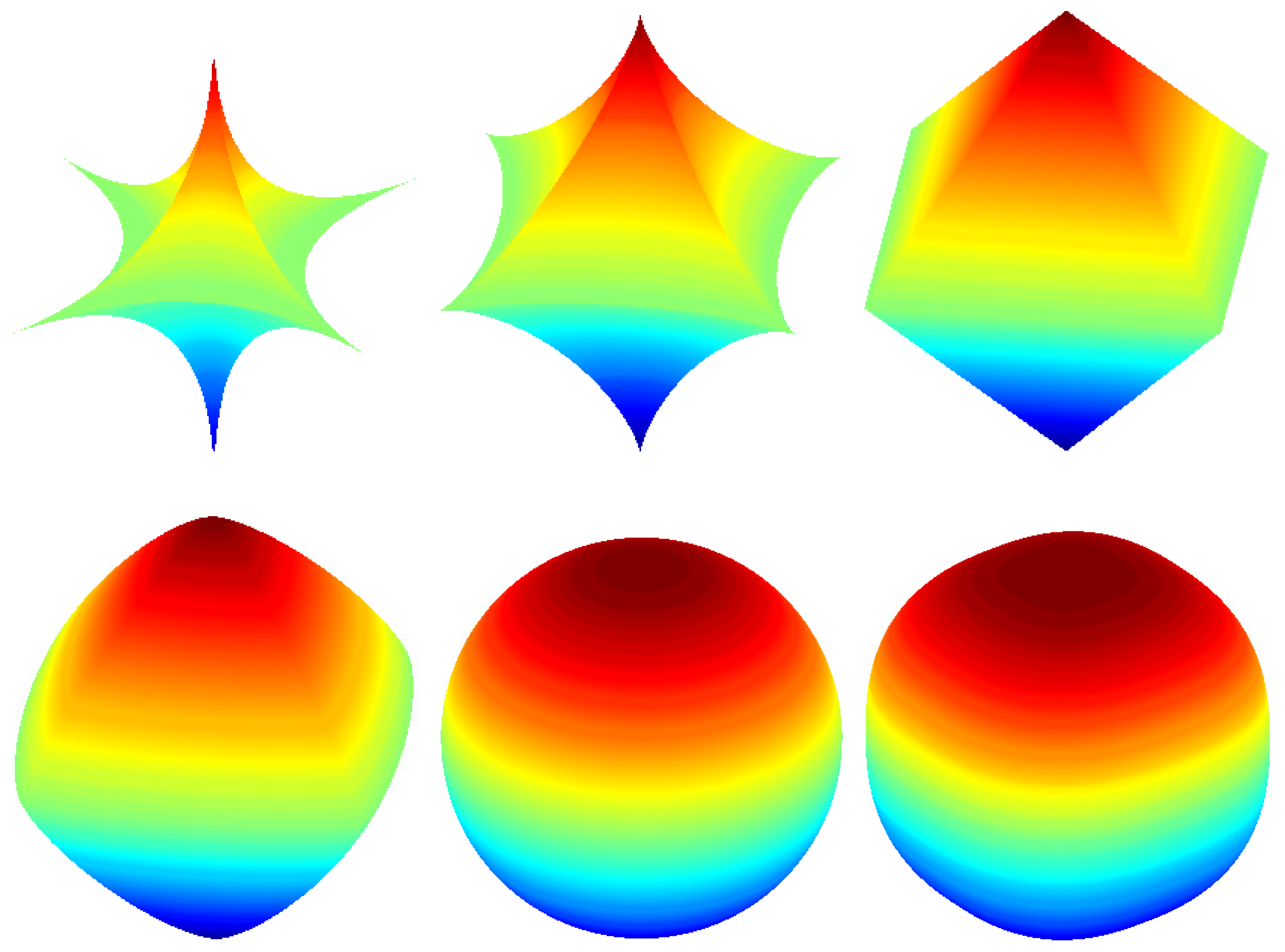
For $p=1$ the ball ${\mathcal{B}}_1\left(r\right)$ is the regular octahedron with the vertices on the axes, at distance r from the origin. For $p=\infty$, the set ${\mathcal{B}}_{\infty }\left(r\right)$ is the cube with edge of length $2r$ and for $p=2$ the region ${\mathcal{B}}_2\left(r\right)$ represents the Euclidean ball. For $p>2$ the balls are called superellipsoids and they are used in computer graphics (see [1,2], where the author uses the name superquadrics to refer to both superellipsoids and supertoroids). Some examples of balls ${\mathcal{B}}_p\left(r\right)$, for different values of p are given in Figure 1.

The volume of the 3D p-ball is

$$\begin{array}{cc}\hfill \mathrm{Vol}\left({\mathcal{B}}_p\left(r\right)\right)& =8{\int }_0^r{\int }_0^{{(r^p-x^p)}^{1/p}}{\int }_0^{{(r^p-x^p-y^p)}^{1/p}}\mathrm{d}z\mathrm{d}y\mathrm{d}x\hfill \\ & =8r^3\frac{{\mathsf{\Gamma }}^3(1/p+1)}{\mathsf{\Gamma }(3/p+1)}.\hfill \end{array}$$

We notice that the radius $r^{\prime }$ of the regular octahedron ${\mathcal{B}}_1\left(r^{\prime }\right)$ with the same volume as the p-ball ${\mathcal{B}}_p\left(r\right)$ must be

$$r^{\prime }=r{c}_p,\mathrm{with}{c}_p=\sqrt[3]{6}\frac{\mathsf{\Gamma }(1/p+1)}{\sqrt[3]{\mathsf{\Gamma }(3/p+1)}}.$$

We will construct a map ${\mathcal{U}}_p:{\mathcal{B}}_p\left(r\right)\to {\mathcal{B}}_1\left(r^{\prime }\right)$ which preserves the volume, i.e., ${\mathcal{U}}_p$ satisfies

$$\mathrm{Vol}\left(D\right)=\mathrm{Vol}\left({\mathcal{U}}_p\left(D\right)\right),\mathrm{for}\mathrm{all}\mathrm{domains}D\subseteq {\mathcal{B}}_p\left(r\right).$$

(2)

Consider the bijections $F_{1,p},F_{2,p}:[0,1]\to [0,1]$, which are particular cases of the regularized incomplete Beta function (also known in statistics as cumulative beta distribution functions)

$$\begin{array}{cc}\hfill F_{1,p}\left(t\right)& =\frac{1}{{\int }_0^1{\left[u(1-u)\right]}^{\frac{1}{p}-1}\mathrm{d}u}{\int }_0^t{u}^{\frac{1}{p}-1}{(1-u)}^{\frac{1}{p}-1}\mathrm{d}u,\mathrm{for}t\in [0,1],\hfill \\ \hfill F_{2,p}\left(t\right)& =\frac{1}{{\int }_0^1{u}^{\frac{2}{p}-1}{(1-u)}^{\frac{1}{p}-1}\mathrm{d}u}{\int }_0^t{u}^{\frac{2}{p}-1}{(1-u)}^{\frac{1}{p}-1}\mathrm{d}u,\mathrm{for}t\in [0,1].\hfill \end{array}$$

In the standard notation we have $F_{1,p}\left(t\right)=I_t(1/p,1/p)$ and $F_{2,p}\left(t\right)=I_t(2/p,1/p)$, where $I_t$ is the so-called regularized incomplete beta function defined as $I_t(\alpha ,\beta )=B(t;\alpha ,\beta )/B(1;\alpha ,\beta )$, with

$$B(t;\alpha ,\beta )={\int }_0^t{u}^{\alpha -1}{(1-u)}^{\beta -1}du,\mathrm{for}\alpha ,\beta >0.$$

One has $F_{1,p}\left(0\right)=F_{2,p}\left(0\right)=0$ and $F_{1,p}\left(1\right)=F_{2,p}\left(1\right)=1$, further $F_{1,p},F_{2,p}$ are increasing functions. Let $G_{1,p},G_{2,p}:[0,1]\to [0,1]$ be the inverses (in Mathematica one can use the command InverseBetaRegularized for the inverses $G_{1,p}$ and $G_{2,p}$) of the functions $F_{1,p}$ and $F_{2,p}$, respectively.

For $a\in (0,\pi /2)$, let

$${\mathcal{B}}_{p,a}\left(r\right)=\left\{(x,y,z)\in {\mathcal{B}}_p\left(r\right),x,y,z\ge 0,xtana\ge y\right\}.$$

Lemma 1.

For $a\in (0,\pi /2)$ we have

$$\mathrm{Vol}\left({\mathcal{B}}_{p,a}\left(r\right)\right)=\frac{1}{8}{F}_{1,p}\left(\frac{{tan}^{p}a}{1+{tan}^{p}a}\right)\mathrm{Vol}\left({\mathcal{B}}_p\left(r\right)\right).$$

Proof. 

The volume of ${\mathcal{B}}_{p,a}\left(r\right)$ can be computed using the double integral

$$\mathrm{Vol}\left({\mathcal{B}}_{p,a}\left(r\right)\right)=\underset{D}{\int \int }{\left(r^p-x^p-y^p\right)}^{1/p}\mathrm{d}x\mathrm{d}y,$$

where $D=\left\{(x,y)\in {\mathbb{R}}^2,x^p+y^p\le r^p,0\le y\le xtana\right\}$. With the change of variables $x={(\rho cost)}^{2/p}$ and $y={(\rho sint)}^{2/p}$ the Jacobian is

$$J={\left(\frac{2}{p}\right)}^2{\rho }^{\frac{4}{p}-1}{(cost)}^{\frac{2}{p}-1}{(sint)}^{\frac{2}{p}-1}$$

and the new domain of integration is

$$\Delta =\left\{(\rho ,t)\in {\mathbb{R}}^2,0\le \rho \le r^{p/2},0\le t\le arctan\left({tan}^{p/2}a\right)\right\}.$$

The volume of ${\mathcal{B}}_{p,a}\left(r\right)$ is

$$\begin{array}{c}\hfill \mathrm{Vol}\left({\mathcal{B}}_{p,a}\left(r\right)\right)=\frac{4}{p^2}{\int }_0^{r^{p/2}}{(r^p-{\rho }^2)}^{\frac{1}{p}}{\rho }^{\frac{4}{p}-1}\mathrm{d}\rho {\int }_0^{arctan\left({tan}^{\frac{p}{2}}a\right)}{(cost)}^{\frac{2}{p}-1}{(sint)}^{\frac{2}{p}-1}\mathrm{d}t.\end{array}$$

With the change of variables $u={\rho }^2/r^p$ and $v={sin}^{2}t$ in the two independent integrals we get

$$\begin{array}{cc}\hfill \mathrm{Vol}\left({\mathcal{B}}_{p,a}\left(r\right)\right)& =\frac{r^3}{p^2}{\int }_0^1{(1-u)}^{\frac{1}{p}}{u}^{\frac{2}{p}-1}\mathrm{d}u{\int }_0^{\frac{{tan}^{p}a}{1+{tan}^{p}a}}{v}^{\frac{1}{p}-1}{(1-v)}^{\frac{1}{p}-1}\mathrm{d}v\hfill \\ & =\frac{r^3}{p^2}B(1/p+1,2/p)B(1/p,1/p)F_{1,p}\left(\frac{{tan}^{p}a}{1+{tan}^{p}a}\right)\hfill \\ & =r^3\frac{{\mathsf{\Gamma }}^3(1/p+1)}{\mathsf{\Gamma }(3/p+1)}{F}_{1,p}\left(\frac{{tan}^{p}a}{1+{tan}^{p}a}\right).\hfill \end{array}$$

□

3. Construction of the Volume Preserving Map ${\mathcal{U}}_p:{\mathcal{B}}_p\left(r\right)\to {\mathcal{B}}_1\left(r^{\prime }\right)$ and Its Inverse

Of course, there is no unique map ${\mathcal{U}}_p$ with the volume preserving property. In this section, we will construct a map ${\mathcal{U}}_p:{\mathcal{B}}_p\left(r\right)\to {\mathcal{B}}_1\left(r^{\prime }\right)$ satisfying the following conditions:

(a)

${\mathcal{U}}_p$ has the volume preserving property (2);

(b)

${\mathcal{U}}_p$ is continuous on ${\mathcal{B}}_p\left(r\right)$ and has continuous partial derivatives at every point of ${\mathcal{B}}_p\left(r\right)$, except the points of the coordinate planes;

(c)

${\mathcal{U}}_p$ has the symmetry property

$${\mathcal{U}}_p(x,y,z)=(sgn\left(x\right)\overline{X},sgn\left(y\right)\overline{Y},sgn\left(z\right)\overline{Z}),\mathrm{where}(\overline{X},\overline{Y},\overline{Z})={\mathcal{U}}_p\left(\right|x|,|y|,|z\left|\right);$$

(d)

${\mathcal{U}}_p$ maps every ${\mathcal{B}}_{p,a}\left(\tilde{r}\right)$ onto some ${\mathcal{B}}_{1,b}\left(c_p\tilde{r}\right)$.

Theorem 2.

The map ${\mathcal{U}}_p=(X,Y,Z)$ with the properties (a)–(d) is defined by

$$\begin{array}{cc}\hfill X& =sgn\left(x\right)c_p{\left({\left|x\right|}^p+{\left|y\right|}^p+{\left|z\right|}^p\right)}^{\frac{1}{p}}\left[1-F_{1,p}\left(\frac{{\left|y\right|}^p}{{\left|x\right|}^p+{\left|y\right|}^p}\right)\right]\sqrt{F_{2,p}\left(\frac{{\left|x\right|}^p+{\left|y\right|}^p}{{\left|x\right|}^p+{\left|y\right|}^p+{\left|z\right|}^p}\right)},\hfill \\ \hfill Y& =sgn\left(y\right)c_p{\left({\left|x\right|}^p+{\left|y\right|}^p+{\left|z\right|}^p\right)}^{\frac{1}{p}}{F}_{1,p}\left(\frac{{\left|y\right|}^p}{{\left|x\right|}^p+{\left|y\right|}^p}\right)\sqrt{F_{2,p}\left(\frac{{\left|x\right|}^p+{\left|y\right|}^p}{{\left|x\right|}^p+{\left|y\right|}^p+{\left|z\right|}^p}\right)},\hfill \\ \hfill Z& =sgn\left(z\right)c_p{\left({\left|x\right|}^p+{\left|y\right|}^p+{\left|z\right|}^p\right)}^{\frac{1}{p}}\left[1-\sqrt{F_{2,p}\left(\frac{{\left|x\right|}^p+{\left|y\right|}^p}{{\left|x\right|}^p+{\left|y\right|}^p+{\left|z\right|}^p}\right)}\right],\hfill \end{array}$$

when${\left|x\right|}^p+{\left|y\right|}^p>0$, and$(X,Y,Z)=(0,0,c_{p}z)$when${\left|x\right|}^p+{\left|y\right|}^p=0$.

Proof. 

Let $(x,y,z)\in {\mathcal{B}}_p\left(r\right)$. Then $(X,Y,Z)={\mathcal{U}}_p(x,y,z)\in {\mathcal{B}}_1\left(r^{\prime }\right)$. Consider first the case $x,y,z>0$. From condition (d) for the limit case $a=\frac{\pi }{2}$ and using (a) and (c) we deduce that $\mathrm{Vol}\left({\mathcal{B}}_p\left(r\right)\right)=\mathrm{Vol}\left({\mathcal{B}}_1\left(c_{p}r\right)\right)$. This relation gives us

$$X+Y+Z=c_p{\left(x^p+y^p+z^p\right)}^{1/p}.$$

(3)

From conditions (a) and (d) there is some $b>0$ such that

$$\mathrm{Vol}\left({\mathcal{B}}_{p,a}\left(\tilde{r}\right)\right)=\mathrm{Vol}\left({\mathcal{B}}_{1,b}\left(c_p\tilde{r}\right)\right).$$

From Lemma 1 we have

$$F_{1,p}\left(\frac{{tan}^{p}a}{1+{tan}^{p}a}\right)\mathrm{Vol}\left({\mathcal{B}}_p\left(\tilde{r}\right)\right)=F_{1,1}\left(\frac{tanb}{1+tanb}\right)\mathrm{Vol}\left({\mathcal{B}}_1\left(c_p\tilde{r}\right)\right).$$

Since ${\mathcal{B}}_p\left(\tilde{r}\right)$ and ${\mathcal{B}}_1\left(c_p\tilde{r}\right)$ have the same volume and $F_{1,1}\left(t\right)=t$ we obtain

$$F_{1,p}\left(\frac{{tan}^{p}a}{1+{tan}^{p}a}\right)=\frac{tanb}{1+tanb}.$$

Further, since $tana=y/x$ and $tanb=Y/X$, this equality can be written as

$$F_{1,p}\left(\frac{y^p}{x^p+y^p}\right)=\frac{Y}{X+Y}.$$

(4)

From conditions (a) and (b) the Jacobian of ${\mathcal{U}}_p$ must be 1, i.e.

$$\left|\begin{array}{ccc}\frac{\partial X}{\partial x}& \frac{\partial X}{\partial y}& \frac{\partial X}{\partial z}\\ \frac{\partial Y}{\partial x}& \frac{\partial Y}{\partial y}& \frac{\partial Y}{\partial z}\\ \frac{\partial Z}{\partial x}& \frac{\partial Z}{\partial y}& \frac{\partial Z}{\partial z}\end{array}\right|=1.$$

(5)

Further, taking into account Formulas (3) and (4) we have

$$\begin{array}{c}Z=c_p{\left(x^p+y^p+z^p\right)}^{1/p}-X-Y,\hfill \\ Y=X{F}_{1,p}\left(\frac{y^p}{x^p+y^p}\right){\left(1-F_{1,p}\left(\frac{y^p}{x^p+y^p}\right)\right)}^{-1},\hfill \end{array}$$

then we calculate the partial derivatives of Y and Z with respect to $x,y$ and z and introduce them in (5). After some calculations, we find that X must be solution of the following first order partial differential equation

$$\frac{\partial X}{\partial x}x{z}^{p-1}+\frac{\partial X}{\partial y}y{z}^{p-1}-\frac{\partial X}{\partial z}(x^p+y^p)=\frac{{(x^p+y^p)}^{\frac{2}{p}}{\left[1-F_{1,p}\left(\frac{y^p}{x^p+y^p}\right)\right]}^{2}B\left(\frac{1}{p},\frac{1}{p}\right)}{c_{p}pX{(x^p+y^p+z^p)}^{\frac{1}{p}-1}}.$$

With $U=X^2$ the equation is rewritten

$$\frac{\partial U}{\partial x}x{z}^{p-1}+\frac{\partial U}{\partial y}y{z}^{p-1}-\frac{\partial U}{\partial z}(x^p+y^p)=2\frac{{(x^p+y^p)}^{\frac{2}{p}}{\left[1-F_{1,p}\left(\frac{y^p}{x^p+y^p}\right)\right]}^{2}B\left(\frac{1}{p},\frac{1}{p}\right)}{c_{p}p{(x^p+y^p+z^p)}^{\frac{1}{p}-1}}.$$

We have to solve the symmetric system

$$\frac{\mathrm{d}x}{x{z}^{p-1}}=\frac{\mathrm{d}y}{y{z}^{p-1}}=\frac{\mathrm{d}z}{-(x^p+y^p)}=\frac{c_{p}p{(x^p+y^p+z^p)}^{\frac{1}{p}-1}\mathrm{d}u}{2{(x^p+y^p)}^{\frac{2}{p}}{\left[1-F_{1,p}\left(\frac{y^p}{x^p+y^p}\right)\right]}^{2}B\left(\frac{1}{p},\frac{1}{p}\right)}.$$

The first equality gives us $y=x{C}_1$, for some constant $C_1$. Replacing this in the equality

$$\frac{\mathrm{d}x}{x{z}^{p-1}}=\frac{\mathrm{d}z}{-(x^p+y^p)}$$

we get $x^p+y^p+z^p=C_2$, for some constant $C_2$. Replacing these two relations in the equality

$$\frac{\mathrm{d}x}{x{z}^{p-1}}=\frac{c_{p}p{(x^p+y^p+z^p)}^{\frac{1}{p}-1}\mathrm{d}u}{2{(x^p+y^p)}^{\frac{2}{p}}{\left[1-F_{1,p}\left(\frac{y^p}{x^p+y^p}\right)\right]}^{2}B\left(\frac{1}{p},\frac{1}{p}\right)},$$

integrating and using that the plane $x=0$ is mapped onto $U=0$ (this follows from the conditions (b) and (c) of the map), we obtain

$$U=\frac{2C_2^{\frac{2}{p}}B(1/p,1/p)B(2/p,1/p)}{p^2{c}_p}{\left[1-F_{1,p}\left(\frac{C_1^p}{1+C_1^p}\right)\right]}^2{F}_{2,p}\left(\frac{x^p(1+C_1^p)}{C_2}\right),$$

which is equivalent to

$$X=c_p{\left(x^p+y^p+z^p\right)}^{1/p}\left[1-F_{1,p}\left(\frac{y^p}{x^p+y^p}\right)\right]\sqrt{F_{2,p}\left(\frac{x^p+y^p}{x^p+y^p+z^p}\right)}.$$

(6)

Then,

$$\begin{array}{c}\hfill Y=c_p{\left(x^p+y^p+z^p\right)}^{1/p}{F}_{1,p}\left(\frac{y^p}{x^p+y^p}\right)\sqrt{F_{2,p}\left(\frac{x^p+y^p}{x^p+y^p+z^p}\right)},\end{array}$$

(7)

$$\begin{array}{c}\hfill Z=c_p{\left(x^p+y^p+z^p\right)}^{1/p}\left[1-\sqrt{F_{2,p}\left(\frac{x^p+y^p}{x^p+y^p+z^p}\right)}\right].\end{array}$$

(8)

In the case when $z=0$ and also in the case when $x=0$ or $y=0$ but $x+y>0$ we use Formulas (6)–(8) to define the map ${\mathcal{U}}_p$. In the case when $x=y=0$, we define ${\mathcal{U}}_p(0,0,z)=(0,0,c_{p}z)$, for all $z\ge 0$, using the continuity property of the map ${\mathcal{U}}_p$.

Finally, for the points $(x,y,z)$ in the other seven octants, the map ${\mathcal{U}}_p$ will be defined as

$${\mathcal{U}}_p(x,y,z)=(sgn\left(x\right)\overline{X},sgn\left(y\right)\overline{Y},sgn\left(z\right)\overline{Z}),\mathrm{where}(\overline{X},\overline{Y},\overline{Z})={\mathcal{U}}_p\left(\right|x|,|y|,|z\left|\right).$$

□

Remark. 

Not all the partial derivatives of the map ${\mathcal{U}}_p$ which occur in Theorem 2 exist at the points of the coordinates planes. For example, $\frac{\partial Y}{\partial x}$ does not exist at the points $(0,y,z)$, because the partial derivative of $F_{1,p}\left(\frac{{\left|y\right|}^p}{{\left|x\right|}^p+{\left|y\right|}^p}\right)$ with respect to x does not exist at the points $(0,y,z)$.

The expression of the inverse map of ${\mathcal{U}}_p$ is given in the next theorem.

Theorem 3.

The map ${\mathcal{U}}_p^{-1}:{\mathcal{B}}_1\left(r^{\prime }\right)\to {\mathcal{B}}_p\left(r\right)$ is defined by

$$x=\frac{X+Y+Z}{c_p}{G}_{1,p}^{\frac{1}{p}}\left(\frac{Y}{X+Y}\right)G_{2,p}^{\frac{1}{p}}\left({\left(\frac{X+Y}{X+Y+Z}\right)}^2\right),$$

(9)

$$y=\frac{X+Y+Z}{c_p}{\left(1-G_{1,p}\left(\frac{Y}{X+Y}\right)\right)}^{\frac{1}{p}}{G}_{2,p}^{\frac{1}{p}}\left({\left(\frac{X+Y}{X+Y+Z}\right)}^2\right),$$

(10)

$$z=\frac{X+Y+Z}{c_p}{\left(1-G_{2,p}\left({\left(\frac{X+Y}{X+Y+Z}\right)}^2\right)\right)}^{\frac{1}{p}},$$

(11)

for every $(X,Y,Z)\in {\mathcal{B}}_1\left(r^{\prime }\right)$ and $X\ge 0$, $Y\ge 0$, $Z\ge 0$, $X+Y>0$. If $X=Y=0$, we have ${\mathcal{U}}_p^{-1}(0,0,Z)=(0,0,Z/c_p)$.

In the other seven octants, we define the inverse of the map ${\mathcal{U}}_p$ using the symmetry property (c) of ${\mathcal{U}}_p$.

Proof. 

Condition (4) is equivalent to

$$\frac{y^p}{x^p+y^p}=G_{1,p}\left(\frac{Y}{X+Y}\right).$$

Replacing (3) in (7) we obtain

$$\frac{X+Y}{X+Y+Z}=\sqrt{F_{2,p}\left(\frac{x^p+y^p}{x^p+y^p+z^p}\right)},$$

which is equivalent to

$$\frac{x^p+y^p}{x^p+y^p+z^p}=G_{2,p}\left({\left(\frac{X+Y}{X+Y+Z}\right)}^2\right).$$

After some computations we can express $x,y,z$ in terms of $X,Y,Z$ to obtain (9)–(11). □

4. Particular Cases

4.1. The Cases $p=1$ and $p=2$

For $p=1$ one has $c_1=1$, $F_{1,p}\left(t\right)=t$ and $F_{2,p}\left(t\right)=t^2,$ therefore ${\mathcal{U}}_1$ is the identity.

For $p=2$ one has $c_2={\pi }^{\frac{1}{3}}$, $F_{1,p}\left(t\right)=\frac{1}{\pi }\left(arcsin(2t-1)+\frac{\pi }{2}\right)=\frac{2}{\pi }arcsin\sqrt{t}$, $F_{2,p}\left(t\right)=1-\sqrt{1-t}$ and for $x,y,z>0$, the map ${\mathcal{U}}_2$ is

$$\begin{array}{c}X=2{\pi }^{-2/3}\sqrt{x^2+y^2+z^2-z\sqrt{x^2+y^2+z^2}}arccos\frac{y}{\sqrt{x^2+y^2}},\hfill \\ Y=2{\pi }^{-2/3}\sqrt{x^2+y^2+z^2-z\sqrt{x^2+y^2+z^2}}arcsin\frac{y}{\sqrt{x^2+y^2}},\hfill \\ Z={\pi }^{1/3}\sqrt{x^2+y^2+z^2}\left(1-\sqrt{1-\frac{z}{\sqrt{x^2+y^2+z^2}}}\right).\hfill \end{array}$$

If we use the spherical coordinates defined by $x=\rho cos\theta sin\phi$, $y=\rho sin\theta sin\phi$ and $z=\rho cos\phi$ we obtain relations (9), (10), (11) from [3], where we also gave the inverse, which has an explicit expression.

4.2. The Case $p=\infty$

In this case we will obtain a new map, different from the one constructed in [4].

We restrict again to the case $x,y,z>0$ because of the symmetry property of the map.

First, a simple calculation shows that $c_{\infty }=6^{1/3}$ and

$$\underset{p\to \infty }{lim}{(x^p+y^p+z^p)}^{1/p}=max(x,y,z).$$

In order to calculate the limits in (6)–(8) when $p\to \infty$ we use the following result.

Lemma 4.

For $\alpha ,\beta >0$ we have

$$\underset{p\to \infty }{lim}\frac{p}{B\left(\frac{\alpha }{p},\frac{\beta }{p}\right)}=\frac{\alpha \beta }{\alpha +\beta }.$$

(12)

Proof. 

We use the equality $\mathsf{\Gamma }\left(x\right)=\mathsf{\Gamma }(x+1)/x$, which holds for $x>0$. One has

$$\frac{p}{B\left(\frac{\alpha }{p},\frac{\beta }{p}\right)}=\frac{p\mathsf{\Gamma }\left(\frac{\alpha +\beta }{p}\right)}{\mathsf{\Gamma }\left(\frac{\alpha }{p}\right)·\mathsf{\Gamma }\left(\frac{\beta }{p}\right)}=\frac{p·\frac{\alpha }{p}·\frac{\beta }{p}·\mathsf{\Gamma }\left(1+\frac{\alpha +\beta }{p}\right)}{\mathsf{\Gamma }\left(1+\frac{\alpha }{p}\right)·\mathsf{\Gamma }\left(1+\frac{\beta }{p}\right)·\frac{\alpha +\beta }{p}},$$

and now it is easy to see that the limit when $p\to \infty$ is the one in (12). □

Proposition 5.

For $x,y,z>0$ we have

$$\begin{array}{ccc}\hfill \underset{p\to \infty }{lim}{F}_{1,p}\left(\frac{y^p}{x^p+y^p}\right)& =& \left\{\begin{array}{cc}\frac{y}{2x},& x>y,\\ 1-\frac{x}{2y},& y\ge x.\end{array}\right.\hfill \end{array}$$

Proof. 

We use the idea in [5].

Suppose $x>y$.

$$F_{1,p}\left(\frac{y^p}{x^p+y^p}\right)=\frac{1}{B\left(\frac{1}{p},\frac{1}{p}\right)}{\int }_0^{y^p/(x^p+y^p)}{\left(u(1-u)\right)}^{\frac{1}{p}-1}\mathrm{d}u.$$

With the change of variable $u=t^p$ we have

$$F_{1,p}\left(\frac{y^p}{x^p+y^p}\right)=\frac{p}{B\left(\frac{1}{p},\frac{1}{p}\right)}{\int }_0^{y/{(x^p+y^p)}^{1/p}}{(1-t^p)}^{\frac{1}{p}-1}\mathrm{d}t.$$

From $0<t<y/(x^p+y^p)$ we further deduce that $x^p/(x^p+y^p)<1-t^p<1$, and therefore

$${\left(\frac{x^p}{x^p+y^p}\right)}^{\frac{1}{p}-1}>{(1-t^p)}^{\frac{1}{p}-1}>1.$$

After integration we obtain

$$\frac{y}{{(x^p+y^p)}^{\frac{1}{p}}}{\left(\frac{x^p}{x^p+y^p}\right)}^{\frac{1}{p}-1}\ge {\int }_0^{y/{(x^p+y^p)}^{1/p}}{(1-t^p)}^{\frac{1}{p}-1}\mathrm{d}t\ge \frac{y}{{(x^p+y^p)}^{\frac{1}{p}}},$$

and further,

$$\frac{p}{B\left(\frac{1}{p},\frac{1}{p}\right)}\frac{y}{{(x^p+y^p)}^{\frac{1}{p}}}{\left(\frac{x^p}{x^p+y^p}\right)}^{\frac{1}{p}-1}\ge F_{1,p}\left(\frac{y^p}{x^p+y^p}\right)\ge \frac{p}{B\left(\frac{1}{p},\frac{1}{p}\right)}\frac{y}{{(x^p+y^p)}^{\frac{1}{p}}}.$$

After applying Lemma 4 for $\alpha =\beta =1$ and replacing the limits

$$\underset{p\to \infty }{lim}{(x^p+y^p)}^{\frac{1}{p}}=max(x,y)=x\mathrm{and}\underset{p\to \infty }{lim}\frac{x^p}{x^p+y^p}=1,$$

□

We finally obtain

$$\underset{p\to \infty }{lim}{F}_{1,p}\left(\frac{y^p}{x^p+y^p}\right)=\frac{y}{2x}.$$

(13)

For the case $y\ge x$ we use the formula $F_{1,p}(1-t)=1-F_{1,p}\left(t\right)$ for $t=x^p/(x^p+y^p)$ and Formula (13), interchanging x and y.

Proposition 6.

For $x,y,z>0$ we have

$$\underset{p\to \infty }{lim}{F}_{2,p}\left(\frac{x^p+y^p}{x^p+y^p+z^p}\right)=\left\{\begin{array}{cc}\hfill \frac{1}{3z^2}max{(x,y)}^2,& \mathrm{if}z=max(x,y,z),\hfill \\ \hfill 1-\frac{2}{3}\frac{z}{max(x,y)},& otherwise.\hfill \end{array}\right.$$

Proof. 

Case 1. Suppose $max(x,y,z)=z$.

With the change of variable $t=u^{2/p}$ we obtain

$$F_{2,p}\left(\frac{x^p+y^p}{x^p+y^p+z^p}\right)=\frac{p}{2B\left(\frac{2}{p},\frac{1}{p}\right)}{\int }_0^{{\left(\frac{x^p+y^p}{x^p+y^p+z^p}\right)}^{2/p}}{\left(1-t^{\frac{p}{2}}\right)}^{\frac{1}{p}-1}\mathrm{d}t.$$

Applying Lemma 4 for $\alpha =2$, $\beta =1$ we have

$$\underset{p\to \infty }{lim}\frac{p}{2B\left(\frac{2}{p},\frac{1}{p}\right)}=\frac{1}{3}.$$

Further, from the condition that t belongs to the interval of integration we can write

$$\frac{z^p}{x^p+y^p+z^p}<1-t^{\frac{p}{2}}<1,$$

and therefore

$${\left(\frac{z^p}{x^p+y^p+z^p}\right)}^{\frac{1}{p}-1}>{\left(1-t^{\frac{p}{2}}\right)}^{\frac{1}{p}-1}>1.$$

After integration we obtain

$${\left(\frac{x^p+y^p}{x^p+y^p+z^p}\right)}^{\frac{2}{p}}{\left(\frac{z^p}{x^p+y^p+z^p}\right)}^{\frac{1}{p}-1}\ge {\int }_0^{{\left(\frac{x^p+y^p}{x^p+y^p+z^p}\right)}^{\frac{2}{p}}}{\left(1-t^{\frac{p}{2}}\right)}^{\frac{1}{p}-1}\mathrm{d}t\ge {\left(\frac{x^p+y^p}{x^p+y^p+z^p}\right)}^{\frac{2}{p}}.$$

A simple calculation shows that

$$\underset{p\to \infty }{lim}{\left(\frac{x^p+y^p}{x^p+y^p+z^p}\right)}^{2/p}=\frac{{(max(x,y))}^2}{z^2}\mathrm{and}\underset{p\to \infty }{lim}\frac{z^p}{x^p+y^p+z^p}=1,$$

which imply that

$$\underset{p\to \infty }{lim}{\int }_0^{{\left(\frac{x^p+y^p}{x^p+y^p+z^p}\right)}^{\frac{2}{p}}}{\left(1-t^{\frac{p}{2}}\right)}^{\frac{1}{p}-1}\mathrm{d}t=\frac{{(max(x,y))}^2}{z^2}.$$

Case 2. Suppose $max(x,y,z)=x$ or y.

Using the equality

$$I_x(\alpha ,\beta )=1-I_{1-x}(\beta ,\alpha ),\alpha ,\beta >0,x\in [0,1],$$

we have

$$F_{2,p}\left(\frac{x^p+y^p}{x^p+y^p+z^p}\right)=1-\frac{1}{B\left(\frac{2}{p},\frac{1}{p}\right)}{\int }_0^{\frac{z^p}{x^p+y^p+z^p}}{u}^{\frac{1}{p}-1}{(1-u)}^{\frac{2}{p}-1}\mathrm{d}u.$$

With the change of variable $u=t^p$ we get

$$F_{2,p}\left(\frac{x^p+y^p}{x^p+y^p+z^p}\right)=1-\frac{p}{B\left(\frac{2}{p},\frac{1}{p}\right)}{\int }_0^{{\left(\frac{z^p}{x^p+y^p+z^p}\right)}^{1/p}}{(1-t^p)}^{\frac{2}{p}-1}\mathrm{d}t.$$

Similarly

$$\frac{z}{{(x^p+y^p+z^p)}^{1/p}}{\left(\frac{x^p+y^p}{x^p+y^p+z^p}\right)}^{\frac{2}{p}-1}\ge {\int }_0^{{\left(\frac{z^p}{x^p+y^p+z^p}\right)}^{1/p}}{(1-t^p)}^{\frac{2}{p}-1}\mathrm{d}t\ge \frac{z}{{(x^p+y^p+z^p)}^{1/p}}.$$

Using

$$\underset{p\to \infty }{lim}\frac{z}{{(x^p+y^p+z^p)}^{1/p}}=\frac{z}{max(x,y)}\mathrm{and}\underset{p\to \infty }{lim}\frac{x^p+y^p}{x^p+y^p+z^p}=1,$$

the proof is complete. □

In conclusion, for $x,y,z>0$, the map ${\mathcal{U}}_{\infty }$ has the values $(X,Y,Z)={\mathcal{U}}_{\infty }(x,y,z)$ given by:

$$\begin{array}{c}\hfill 6^{1/3}\left(\frac{x}{2\sqrt{3}},\frac{2y-x}{2\sqrt{3}},z-\frac{y}{\sqrt{3}}\right),x\le y\le z,\\ \hfill 6^{1/3}\left(\frac{x}{2}\sqrt{1-\frac{2z}{3y}},\left(y-\frac{x}{2}\right)\sqrt{1-\frac{2z}{3y}},y\left(1-\sqrt{1-\frac{2z}{3y}}\right)\right),x\le z\le y,\\ \hfill 6^{1/3}\left(\frac{2x-y}{2\sqrt{3}},\frac{y}{2\sqrt{3}},z-\frac{x}{\sqrt{3}}\right),y\le x\le z,\\ \hfill 6^{1/3}\left(\left(x-\frac{y}{2}\right)\sqrt{1-\frac{2z}{3x}},\frac{y}{2}\sqrt{1-\frac{2z}{3x}},x\left(1-\sqrt{1-\frac{2z}{3x}}\right)\right),y\le z\le x,\\ \hfill 6^{1/3}\left(\frac{x}{2}\sqrt{1-\frac{2z}{3y}},\left(y-\frac{x}{2}\right)\sqrt{1-\frac{2z}{3y}},y\left(1-\sqrt{1-\frac{2z}{3y}}\right)\right),z\le x\le y,\\ \hfill 6^{1/3}\left(\left(x-\frac{y}{2}\right)\sqrt{1-\frac{2z}{3x}},\frac{y}{2}\sqrt{1-\frac{2z}{3x}},x\left(1-\sqrt{1-\frac{2z}{3x}}\right)\right),z\le y\le x,\end{array}$$

and can be reduced to

$$\begin{array}{c}\hfill 6^{1/3}\left(\frac{x}{2\sqrt{3}},\frac{2y-x}{2\sqrt{3}},z-\frac{y}{\sqrt{3}}\right),x\le y\le z,\\ \hfill 6^{1/3}\left(\frac{x}{2}\sqrt{1-\frac{2z}{3y}},\left(y-\frac{x}{2}\right)\sqrt{1-\frac{2z}{3y}},y\left(1-\sqrt{1-\frac{2z}{3y}}\right)\right),x\le y,z\le y,\\ \hfill 6^{1/3}\left(\frac{2x-y}{2\sqrt{3}},\frac{y}{2\sqrt{3}},z-\frac{x}{\sqrt{3}}\right),y\le x\le z,\\ \hfill 6^{1/3}\left(\left(x-\frac{y}{2}\right)\sqrt{1-\frac{2z}{3x}},\frac{y}{2}\sqrt{1-\frac{2z}{3x}},x\left(1-\sqrt{1-\frac{2z}{3x}}\right)\right),y\le x,z\le x.\end{array}$$

The above formulas can also be used in the case when $x=0$ or $y=0$ or $z=0$, with the mention that the denominators cannot be zero, except the case when $x=y=z=0$, when we take ${\mathcal{U}}_{\infty }(0,0,0)=(0,0,0).$

After some calculations we get that, for $X,Y,Z>0$ the inverse ${\mathcal{U}}_{\infty }^{-1}(X,Y,Z)$ is given by

$$\begin{array}{c}\hfill 6^{-1/3}\left(2\sqrt{3}X,\sqrt{3}(X+Y),X+Y+Z\right),\mathrm{on}{D}_1,\\ \hfill 6^{-1/3}\left(\frac{2X(X+Y+Z)}{X+Y},X+Y+Z,\frac{3Z(2X+2Y+Z)}{2(X+Y+Z)}\right),\mathrm{on}{D}_2,\\ \hfill 6^{-1/3}\left(\sqrt{3}(X+Y),2\sqrt{3}Y,X+Y+Z\right),\mathrm{on}{D}_3,\\ \hfill 6^{-1/3}\left(X+Y+Z,\frac{2Y(X+Y+Z)}{X+Y},\frac{3Z(2X+2Y+Z)}{2(X+Y+Z)}\right),\mathrm{on}{D}_4,\end{array}$$

where $D_i,i=1,2,3,4$ are the set of points $(X,Y,Z)$ satisfying the following conditions, respectively:

$$\begin{array}{c}\hfill X\le Y,\sqrt{3}(X+Y)\le X+Y+Z,\\ \hfill X\le Y,\frac{3Z(2X+2Y+Z)}{2(X+Y+Z)}\le X+Y+Z,\\ \hfill Y\le X,(X+Y)\sqrt{3}\le X+Y+Z,\\ \hfill Y\le X,\frac{3Z(2X+2Y+Z)}{2(X+Y+Z)}\le X+Y+Z.\end{array}$$

Condition

$$\frac{3Z(2X+2Y+Z)}{2(X+Y+Z)}\le X+Y+Z$$

can be written as $3({(X+Y+Z)}^2-{(X+Y)}^2)\le 2{(X+Y+Z)}^2,$ and is equivalent to $X+Y+Z\le \sqrt{3}(X+Y)$, since $X,Y,Z>0$.

Therefore,

$$\begin{array}{c}\hfill D_1=\{X\le Y,\sqrt{3}(X+Y)\le X+Y+Z\},\\ \hfill D_2=\{X\le Y,X+Y+Z\le \sqrt{3}(X+Y)\},\\ \hfill D_3=\{Y\le X,(X+Y)\sqrt{3}\le X+Y+Z\},\\ \hfill D_4=\{Y\le X,X+Y+Z\le \sqrt{3}(X+Y)\}.\end{array}$$

Finally, the expressions of $(x,y,z)={\mathcal{U}}_{\infty }^{-1}(X,Y,Z)$ can be reduced to

$$\begin{array}{c}x=6^{-1/3}min\left(\sqrt{3},1+\frac{Z}{X+Y}\right)\left(X+min(X,Y)\right),\hfill \\ y=6^{-1/3}min\left(\sqrt{3},1+\frac{Z}{X+Y}\right)\left(Y+min(X,Y)\right),\hfill \\ z=6^{-1/3}min\left(X+Y+Z,3Z\left(1-\frac{Z}{2(X+Y+Z)}\right)\right).\hfill \end{array}$$

These formulas can also be used in the case when $Z=0$ and in the case when $X=0$ or $Y=0$, but $X+Y>0$. In the case when $X=Y=0$ we take ${\mathcal{U}}_{\infty }^{-1}(0,0,Z)=(0,0,6^{-1/3}Z)$.

If we take arbitrary numbers $p,\tilde{p}>0$, the application

$${\mathcal{U}}_{\tilde{p}}^{-1}\circ {\mathcal{U}}_p:{\mathcal{B}}_p\left(r\right)\to {\mathcal{B}}_{\tilde{p}}\left(\tilde{r}\right),\mathrm{with}\tilde{r}=c_p{c}_{\tilde{p}}^{-1}r,$$

is a volume preserving map, therefore we have defined a volume preserving map between arbitrary p-balls.

5. Possible Applications

A uniform grid of a 3D domain D is a grid in which all the cells have the same volume. This is required in statistical applications, in computer graphics in the theory of deformable bodies (see, for example, Ref. [6] and the references therein) and in construction of wavelet bases of the space $L^2\left(D\right)$. A refinement process is needed for multiresolution analysis or for multigrid methods, when a grid is not fine enough to solve a problem accurately. A refinement of a 3D grid is called uniform when each cell is divided into a given number of smaller cells having the same volume. To be efficient in practice, a refinement procedure should also be a simple one. One efficient way to construct a uniform and refinable (UR) grid on a domain D is to map on D an existing UR grid by a volume preserving map. In our case, we can construct (UR) grids on a ball ${\mathcal{B}}_{p^{\prime }}$ by transporting from a ball ${\mathcal{B}}_p$ an already constructed (UR) grid. The simplest example of such a ball with (UR) grids is the cube ${\mathcal{B}}_{\infty }$, but we have also constructed such (UR) grids on the regular octahedron ${\mathcal{B}}_1$ (see [3,4]) and on the 3D Euclidean ball ${\mathcal{B}}_2$ (see [3,7] ).

The technique used in [3] can be easily adapted to the p-ball ${\mathcal{B}}_p$ in order to construct multiresolution analysis of $L^2\left({\mathcal{B}}_p\right)$ and orthonormal wavelet bases on the p-ball ${\mathcal{B}}_p$.

The centers of the cells in our (UR) grids in ${\mathcal{B}}_p$ can be taken as points in interpolation formulas, as Monte Carlo interpolation or adaptive interpolation formulas.

Another application of volume preserving maps is in the theory of partial differential equations on Lipschitz domains (see [8]).

References

1. Barr, A.H. Superquadrics and Angle-Preserving Transformations. IEEE-CGA 1981, 1, 11–23. [Google Scholar] [CrossRef]
2. Barr, A.H. Rigid Physically Based Superquadrics. In Graphics Gems III; Kirk, D., Ed.; Academic Press: San Diego, CA, USA, 1992; pp. 137–159. [Google Scholar]
3. Holhoş, A.; Roşca, D. Orhonormal Wavelet Bases on the 3D Ball via Volume Preserving Map from the Regular Octahedron. Available online: https://arxiv.org/abs/1910.08067 (accessed on 10 October 2019).
4. Holhoş, A.; Roşca, D. Uniform refinable 3D grids of regular convex polyhedrons and balls. Acta Math. Hung. 2018, 156, 182–193. [Google Scholar] [CrossRef]
5. Holhoş, A. Two Area Preserving Maps from the Square to the p-Ball. Math. Modell. Anal. 2017, 22, 157–166. [Google Scholar] [CrossRef]
6. Savoye, Y. Cage-Based Performance Capture; Springer: Basel, Switzerland, 2014. [Google Scholar]
7. Roşca, D.; Morawiec, A.; De Graef, M. A new method of constructing a grid in the space of 3D rotations and its applications to texture analysis. Model. Simul. Mater. Sci. Eng. 2014, 22, 075013. [Google Scholar] [CrossRef]
8. Griepentrog, J.; Höpner, W.; Kaiser, H.C.; Rehberg, J. A bi-Lipschitz continuous, volume preserving map from the unit ball onto a cube. Note Mat. 2008, 28, 177–193. [Google Scholar]
Figure 1. Some balls B p ( r ) for p = 0.5 , p = 0.75 , p = 1 (first line) and p = 1.2 , p = 2 and p = 2.5 (second line), respectively.
Symmetry 11 01404 g001