Acquiring the Symplectic Operator Based on Pure Mathematical Derivation Then Verifying It in the Intrinsic Problem of Nanodevices

Abstract

The symplectic algorithm can maintain the symplectic structure and intrinsic properties of the system, its cumulative error is small and suitable for multi-step calculation. At present, the widely accepted symplectic operators are obtained by solving the Hamilton equation based on artificial definitions and assumptions in advance. There are inevitable dispersion errors. We solve the equation by pure mathematical derivation without any artificial limitations and assumptions. The way to accurately obtain high-precision symplectic operators greatly reduces the dispersion error from the beginning. The numerical solution of the one-dimensional Schrödinger equation for describing the intrinsic problem of nanodevices is used as an application environment to compare the total energy distribution of the particle wave function in the box, thus verifying the properties of the Symplectic Operator based on Pure Mathematical Derivation by comparing with Finite-Difference Time-Domain (FDTD) and the widely accepted symplectic operator.

1. Introduction

The Hamilton system includes pharmacology, structural biology, semiconductors, superconductivity, plasma, celestial mechanics, materials, and partial differential equations. In the study of the Hamiltonian system, there are three efficient methods namely: Finite-Difference Time-Domain (FDTD), Runge–Kutta algorithm, and symplectic algorithms. The Runge–Kutta algorithm is the most widely used method, but its order has certain limitations, and the stability decreases with the increase of the order [1]. Although FDTD is also widely used, the calculation accuracy is low [2] and the time-space stability factor must satisfy a specific condition. Moreover, its numerical stability must be affected by the changes of dielectric constant in different media [3]. Compared with the traditional non-symplectic algorithm, the symplectic algorithm not only has higher precision, but also maintains the symplectic structure of the system without the infinite accumulation of energy errors. Those characteristics are greatly beneficial for solving equations.

There are many ways to achieve the symplectic algorithm. The FDTD method starts from the Maxwell equations that summarize the basic laws of macroscopic electromagnetic fields, and makes full use of the accuracy of finite difference to achieve accurate solution of electromagnetic problems. The FDTD method is very convenient for electromagnetic modeling of complex targets and has been widely used in solving electromagnetic problems such as electromagnetic propagation, radiation, and scattering.

We start from Maxwell’s equations and get it in Cartesian coordinates.

$$\begin{gathered} \frac{\partial H_x}{\partial t}=\frac{1}{\mu }\left(\frac{\partial E_x}{\partial z}-\frac{\partial E_z}{\partial y}-\rho H_x\right) \\ \frac{\partial H_y}{\partial t}=\frac{1}{\mu }\left(\frac{\partial E_z}{\partial x}-\frac{\partial E_x}{\partial z}-\rho H_y\right) \\ \frac{\partial H_z}{\partial t}=\frac{1}{\mu }\left(\frac{\partial E_x}{\partial y}-\frac{\partial E_y}{\partial x}-\rho H_z\right) \\ \frac{\partial E_x}{\partial t}=\frac{1}{\mu }\left(\frac{\partial H_x}{\partial z}-\frac{\partial H_z}{\partial y}-\rho E_x\right) \\ \frac{\partial E_y}{\partial t}=\frac{1}{\mu }\left(\frac{\partial H_z}{\partial x}-\frac{\partial H_x}{\partial z}-\rho E_y\right) \\ \frac{\partial E_z}{\partial t}=\frac{1}{\mu }\left(\frac{\partial H_x}{\partial y}-\frac{\partial H_y}{\partial x}-\rho E_z\right) \end{gathered}$$

These six coupled partial differential equations are the basis of the FDTD algorithm, where E and H represent the electric field strength and the magnetic field strength, respectively. In the FDTD method, the time step Δt and the spatial step size Δx Δy Δz are not independent of each other, and their values must conform to a certain relationship.

It can be inferred that in order to ensure numerical stability, each discrete parameter should satisfy

$$\Delta t\le \frac{1}{\sqrt{\frac{1}{{\left(\Delta x\right)}^2}+\frac{1}{{\left(\Delta y\right)}^2}+\frac{1}{{\left(\Delta z\right)}^2}}}$$

This is the numerical stability condition of the FDTD algorithm, which gives the relationship that should be satisfied between space and time interval.

Ruth [4] proposed a method for calculating the third-order symplectic algorithm equation in 1983. Ruth considered a system of differential equations governed by the Hamiltonian,

$$H=\frac{{\overrightarrow{p}}^2}{2}+v\left(\overrightarrow{x},t\right)$$

He also developed an explicit third-order symplectic map and to indicate the method for higher order maps. He let the approximate nth order symplectic map be denoted by $\left(\mathrm{x},\mathrm{p}\right)={\mathrm{m}}_{\mathrm{n}}\left(\mathrm{t}\right)\left({\mathrm{x}}_0,{\mathrm{p}}_0\right)$, where t is the time step (assumed small) and n is the order of the map

$$\Vert M\left(T\right)-M_n\left(t\right)\Vert =0\left(t^{n+1}\right)$$

Then he demonstrated a method for finding $M_n\left(t\right)$.

This method is the foundation for the development of the symplectic algorithm. The dispersion characteristics are not suitable to higher-order computational equations. Iwatsu [5] and Cui et al. [6] considered the deficiencies of the Runge–Kutta method by limiting the range of a particular symplectic operator to determine other parameters, this method still cannot efficiently reduce the error to get accurate results. In order to achieve the symplectic method for stochastic Hamiltonian systems with multiplicative noise, Milstein et al. [7] proposed a new class of completely implicit methods for stochastic systems. The increment of the Wiener process in these completely implicit schemes is replaced by some truncated random variables. Mcmahon et al. [8] constructed different integrators based on the selection of discrete Lagrangian for approximation actions, which is beneficial for construction by combining discrete Lagrangian quantities in the explicit symplectic Runge–Kutta method. Xiao et al. [9] developed an explicit high-order, non-classical symplectic algorithm for an ideal two-fluid system. In this method, the fluid is discretized into particles, and the electromagnetic field and internal energy are regarded as discrete differential form fields on a fixed grid. It is suitable for large-scale simulation of large-scale physical problems and requires long-term fidelity and accuracy. Wen [10] defined a hidden symplectic format by using the finite term of the series to approximate the original generation functional in the Hamiltonian system, but it can only restore the physical process more completely and does not explore the huge application of the symplectic algorithm in application research. Qing et al. [11] applied the symplectic algorithm to the analysis of cracks without considering the stable hybrid scheme used in non-traditional solutions or classical hybrid models, nor extending the method to the 2D domain.

In the study of the intrinsic problem of nanodevices, Liang et al. [12] used the variational method to solve the Schrödinger equation, Feng [13] studied the characteristics of He~+ high-order harmonic radiation under butterfly metal nanostructures by numerically solving Schrödinger equation theory. These methods have strict requirements for the accuracy of the solution. Cheng et al. [14] considered the surface polarization effect for nanocrystal quantum dots in discrete background media and applied the perturbation method to solve the Schrödinger equation of excitons. This requires a smaller error range for the analytical solution. Liu et al. [15] conducted a theoretical study on the relationship between the semiconductor surface barrier and the surface energy level and derived the eigenequation of the surface electron wave function energy using the Schrödinger equation and matrix theory. Given the nonlinear relationship between the surface barrier and the surface energy level, it is necessary to use the exact analytical solution to give the simulation curve of the surface energy level solution set under different surface barriers.

How to achieve accurate high-order symplectic operators with minimum error is a difficult problem. Based on the above factors, we propose a method to acquire the symplectic operator based on pure mathematical derivation. We propose a method for accurately calculating symplectic operators by using the correspondence between coefficients of different series and order. This method establishes the corresponding equations and solves them by purely mathematical derivation, using the same unknown symplectic operator to represent other coefficients. The value of the error is minimized to obtain the exact value of the symplectic operator, and the symplectic operator with the best numerical dispersion characteristics is calculated.

2. Materials and Methods

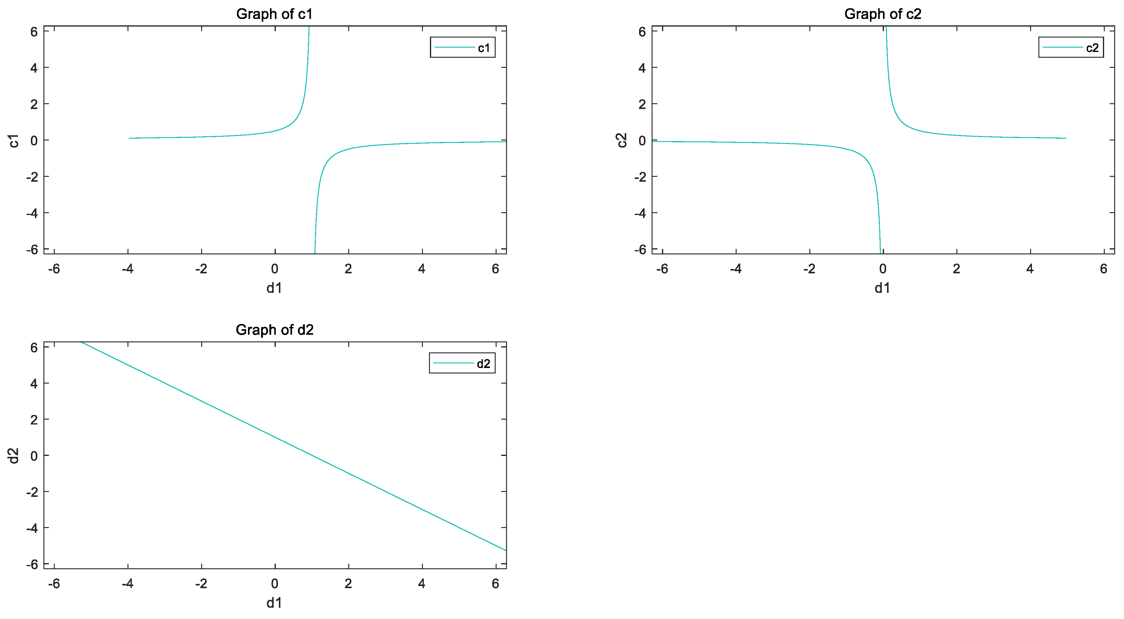
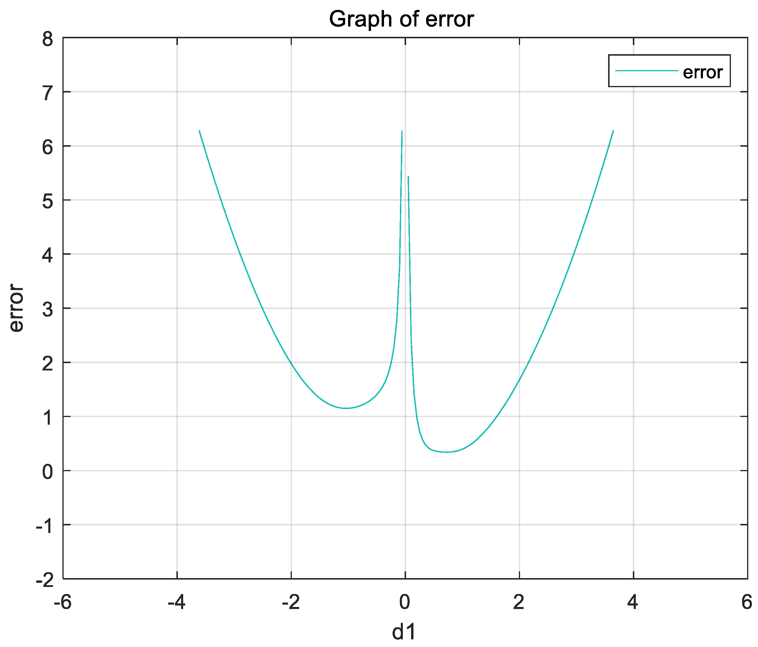
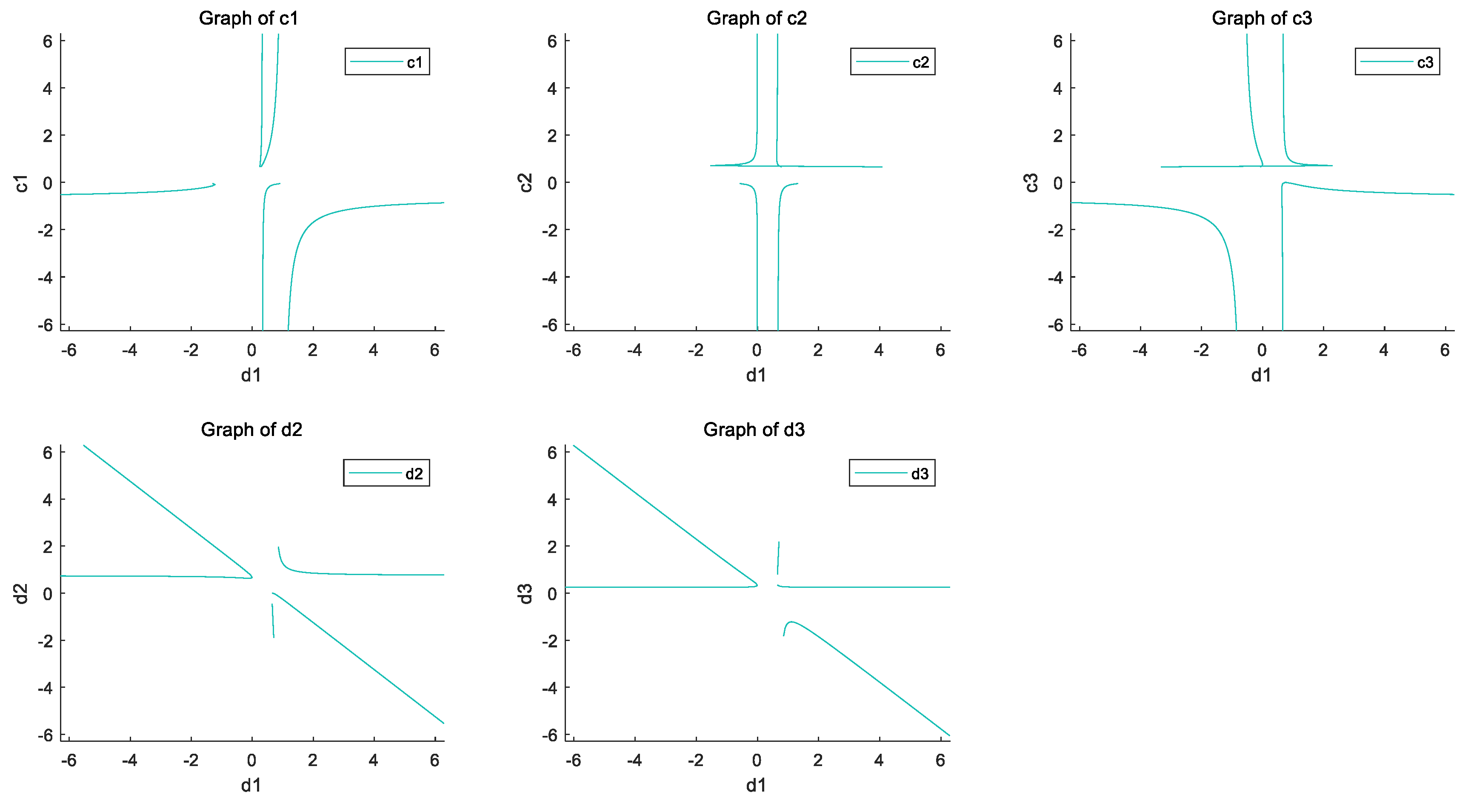
2.1. Calculate Symplectic Operators

The general expression of the Hamilton equation is [16]

$$\frac{dZ}{dt}=J^{-1}{H}_Z=\left\{Z,H\left(Z\right)\right\}=\frac{\partial Z}{\partial q}\frac{\partial H}{\partial p}-\frac{\partial Z}{\partial p}\frac{\partial H}{\partial q}$$

(1)

where $J=\left[\begin{array}{cc}{0}_n& I_n\\ -I_n& 0_n\end{array}\right]$ is the standard symplectic matrix, $0_n,I_n$ are n order 0 matrix and n order unit matrix, $H=H\left(p_1,p_2,\cdots ,p_n,q_1,q_2,\cdots ,q_n\right)$ is the Hamilton function independent of time t, Z is the transposed matrix of H, and the differential operator is introduced.

$$D_H=\mathrm{U}+\mathrm{V},D_{H}Z=\left\{Z,H\right\},$$

Then within ${\Delta }_t$ time interval, $Z\left(\tau \right)=\exp [{\Delta }_t\left(U+V\right)]Z\left(0\right)$. In the symplectic propagator technique, we use the non-dissipative m-level p-order explicit symplectic integral to approximate the time evolution matrix of the Maxwell’s curl equation.

$$\exp \left[{\Delta }_t\left(U+V\right)\right]={\displaystyle \prod }_{l=1}^m\exp \left(d_l{\Delta }_{t}V\right)\exp \left(c_l{\Delta }_{t}U\right)+O\left({\Delta }_t^{p+1}\right)$$

(2)

where $d_l$ and $c_l$ are symplectic operator or symplectic propagator coefficients, and each step of time $\exp \left(c_l{\Delta }_{t}U\right)$ and $\exp \left(d_l{\Delta }_{t}V\right)$ is a basic symplectic transformation.

In order to determine the symplectic operator, we perform Taylor series expansion on the 0 point, then there is

$$\mathrm{LHS}=1+{\Delta }_t\left(U+V\right)+\frac{{\Delta }_t^2}{2!}{\left(U+V\right)}^2+\frac{{\Delta }_t^3}{3!}{\left(U+V\right)}^3+\dots +\frac{{\Delta }_t^p}{p!}{\left(U+V\right)}^p+\frac{{\Delta }_t^{\left(p+1\right)}}{\left(p+1\right)!}{\left(U+V\right)}^{\left(p+1\right)}$$

(3)

$$\begin{array}{cc}\hfill \mathrm{RHS}& ={\displaystyle {\displaystyle \prod }_{l=1}^m}\exp \left(d_l{\Delta }_{t}V\right)\exp (c_l{\Delta }_{t}U)\hfill \\ & =1+{\Delta }_t\left({\displaystyle {\displaystyle \sum }_{i=1}^m}{c}_{i}U+{\displaystyle {\displaystyle \sum }_{j=1}^m}{d}_{j}V\right)+\frac{{\Delta }_t^2}{2!}{\left({\displaystyle {\displaystyle \sum }_{i=1}^m}{c}_{i}U+{\displaystyle {\displaystyle \sum }_{j=1}^m}{d}_{j}V\right)}^2+\dots \hfill \\ & +\frac{{\Delta }_t^p}{p!}{\left({\displaystyle {\displaystyle \sum }_{i=1}^m}{c}_{i}U+{\displaystyle {\displaystyle \sum }_{j=1}^m}{d}_{j}V\right)}^p+\frac{{\Delta }_t^{\left(p+1\right)}}{\left(p+1\right)!}{\left({\displaystyle {\displaystyle \sum }_{i=1}^m}{c}_{i}U+{\displaystyle {\displaystyle \sum }_{j=1}^m}{d}_{j}V\right)}^{\left(p+1\right)}\hfill \\ & =1+{\Delta }_t\left({\displaystyle {\displaystyle \sum }_{i=1}^m}{c}_{i}U+{\displaystyle {\displaystyle \sum }_{j=1}^m}{d}_{j}V\right)\hfill \\ & +\frac{{\Delta }_t^2}{2!}[{\left({\displaystyle {\displaystyle \sum }_{i=1}^l}{c}_i\right)}^2{U}^2+2{\displaystyle {\displaystyle \sum }_{i=1}^l}{c}_i{\displaystyle {\displaystyle \sum }_{j=1}^i}{d}_{j}UV+2{\displaystyle {\displaystyle \sum }_{i=1}^l}{c}_i{\displaystyle {\displaystyle \sum }_{j=i+1}^m}{d}_{j}UV+{\left({\displaystyle {\displaystyle \sum }_{j=1}^m}{d}_j\right)}^2{V}^2]\hfill \\ & +\dots \hfill \end{array}$$

(4)

Comparing the coefficients in the LHS and RHS equations, we can get different order symplectic operators, where the second-order RHS coefficients are expressed as:

$$\begin{gathered} U^2:{\left({\displaystyle \sum }_{i=1}^2{c}_i\right)}^2,V^2:{\left({\displaystyle \sum }_{i=1}^2{d}_l\right)}^2,UV:c_1{d}_2,VU:c_1{d}_1+c_2\left(d_1+d_2\right) \\ {e}_{2,1}={\displaystyle \sum }_{i=1}^l{c}_i{\displaystyle \sum }_{j=1}^i{d}_j-\frac{1}{2},e_{2,2}={\displaystyle \sum }_{i=1}^l{c}_i{\displaystyle \sum }_{j=i+1}^m{d}_j-\frac{1}{2} \end{gathered}$$

Define the error function as

$$\mathrm{error}=\sqrt[2]{\left(e_{3,1}^2+e_{3,2}^2+e_{3,3}^2+\dots +e_{3,5}^2+e_{3,6}^2\right)}$$

$e_{\mathrm{m},\mathrm{n}}^2$ represents the coefficient term of the corresponding symplectic operator.

$$\begin{gathered} e_{3,1}=\frac{1}{2}\left[d_1^1{c}_1^2+d_2\left(c_1+c_2\right)+d_3{\left(c_1+c_2+c_3\right)}^2\right]-\frac{1}{6} \\ {e}_{3,1}=\frac{1}{2}\left[d_1^2{c}_1+d_2^2{c}_2+d_3^2{c}_3\right]-\frac{1}{6} \\ {e}_{3,1}=\frac{1}{2}\left[d_2{\left(c_2+c_3\right)}^2+d_2{c}_3^2\right]-\frac{1}{6} \\ {e}_{3,1}=\frac{1}{2}\left[d_1{c}_2+c_3{\left(d_1+d_2\right)}^2\right]-\frac{1}{6} \\ {e}_{3,1}=\left[d_1\left(c_2+c_3\right)+d_2{d}_3\right]\left(c_1+c_2+c_3\right)-\frac{1}{6} \\ {e}_{3,1}=d_3\left[c_3\left(d_1+d_2\right)+c_2{d}_1\right]+d_2{c}_1{d}_1-\frac{1}{6} \end{gathered}$$

In Figure 1, $c_1,c_2,$ and $d_2$ are represented with $d_1$. It can be seen that $c_1,c_2,$ and $d_2$ vary linearly with the change of $d_1$. Figure 2 shows the variation of the error function with $d_1$. It can be seen that the minimum value of the error function is in the range of $d_1$.

The third-order RHS coefficients are

$$\begin{gathered} U^3:{\left({\displaystyle \sum }_{i=1}^3{c}_i\right)}^3,V^3:{\left({\displaystyle \sum }_{i=1}^3{d}_l\right)}^3,U^2{V}^1:d_1^1{c}_1^2+d_2\left(c_1+c_2\right)+d_3{\left(c_1+c_2+c_3\right)}^2, \\ {U}^1{V}^2:d_1^2{c}_1+d_2^2{c}_2+d_3^2{c}_3,V^1{U}^2:d_2{\left(c_2+c_3\right)}^2+d_2{c}_3^2,V^2{U}^1:d_1{c}_2+c_3{\left(d_1+d_2\right)}^2, \\ {U}^1{V}^1{U}^1:\left[d_1\left(c_2+c_3\right)+d_2{d}_3\right]\left(c_1+c_2+c_3\right), \\ {V}^1{U}^1{V}^1:d_3\left[c_3\left(d_1+d_2\right)+c_2{d}_1\right]+d_2{c}_1{d}_1 \end{gathered}$$

After exact calculation, the relationship between each symplectic operator and d₁ is

$$\begin{gathered} c_1=\frac{2d_1-\frac{3\left[\sqrt{\frac{d_1^1\left(48d_1^3-72d_1^2+39d_1^1-8\right)}{2}}-5d_1^1+4d_1^2+2\right]}{2\left(4d_1^2-3\right)}+2d_1^2+\frac{2d_1\left[\sqrt{\frac{d_1^1\left(48d_1^3-72d_1^2+39d_1^1-8\right)}{2}}-5d_1^1+4d_1^2+2\right]}{4d_1^1-3}}{6d_1^2+4d_1^2} \\ {c}_2=-\frac{d_1^1-\frac{3\left[\sqrt{\frac{d_1^1\left(48d_1^3-72d_1^2+39d_1^1-8\right)}{3}}-5d_1^1+4d_1^2+2\right]}{2\left(4d_1^1-3\right)}+\frac{2d_1^1\left[\sqrt{\frac{d_1^1\left(48d_1^3-72d_1^2+39d_1^1-8\right)}{3}}\right]}{4d_1^1-3}-1}{6d_1^2+4d_1^2} \\ {c}_3=-\frac{5d_1^1-\frac{9\left[\sqrt{\frac{d_1^1\left(48d_1^3-72d_1^2+39d_1^1-8\right)}{3}}-5d_1^1+4d_1^2+2\right]-12d_1^2+\frac{12d_1^1\left[\sqrt{\frac{d_1^1\left(48d_1^3-72d_1^2+39d_1^1-8\right)}{3}}-5d_1^1+4d_1^1+2\right]}{4d_1^1-3}}{4d_1^1-3}}{18d_1^2-8} \\ {d}_1=d_1 \\ {d}_2=\frac{\sqrt{\frac{d_1^1\left(48d_1^3-72d_1^2+39d_1^1-8\right)}{3}}-5d_1^1+4d_1^2+2}{2\left(4d_1^2-3\right)}-d_1^1+1 \\ {d}_3=\frac{\sqrt{\frac{d_1^1\left(48d_1^3-72d_1^2+39d_1^1-8\right)}{3}}+5d_1^1-4d_1^2-2}{2\left(4d_1^2-3\right)} \end{gathered}$$

The relationship between each symplectic operator and d₁ is shown in Figure 3.

In the fourth-order, each symplectic operator constitutes 14 equations, which are

$$\begin{array}{l}{{\displaystyle U}}^3{{\displaystyle V}}^1,{{\displaystyle U}}^1{{\displaystyle V}}^3,{{\displaystyle V}}^3{{\displaystyle U}}^1,{{\displaystyle V}}^1{{\displaystyle U}}^3,\\ {{\displaystyle U}}^2{{\displaystyle V}}^2,{{\displaystyle V}}^2{{\displaystyle U}}^2,{{\displaystyle U}}^2{{\displaystyle V}}^1{{\displaystyle U}}^1,\\ {{\displaystyle U}}^1{{\displaystyle V}}^2{{\displaystyle U}}^1,{{\displaystyle U}}^1{{\displaystyle V}}^1{{\displaystyle U}}^2,\\ {{\displaystyle V}}^1{{\displaystyle U}}^2{{\displaystyle V}}^1,{{\displaystyle V}}^2{{\displaystyle U}}^1{{\displaystyle V}}^1,{{\displaystyle V}}^1{{\displaystyle U}}^1{{\displaystyle V}}^2,\\ {{\displaystyle U}}^1{{\displaystyle V}}^1{{\displaystyle U}}^1{{\displaystyle V}}^1,{{\displaystyle V}}^1{{\displaystyle U}}^1{{\displaystyle V}}^1{{\displaystyle U}}^1\\ \end{array}$$

Which defines the error function as

$$\mathrm{error}=\sqrt{\left(e_{4,1}^2+e_{4,2}^2+e_{4,3}^2+\dots +e_{4,13}^2+e_{4,14}^2\right)}$$

The calculation method is similar to the previous one, and it is omitted here for reasons of space. From the above results, we can get the exact symplectic propagation coefficient through numerical calculation, and at this time, the unique symplectic operator of the system is optimal, and the error function can obtain the minimum value.

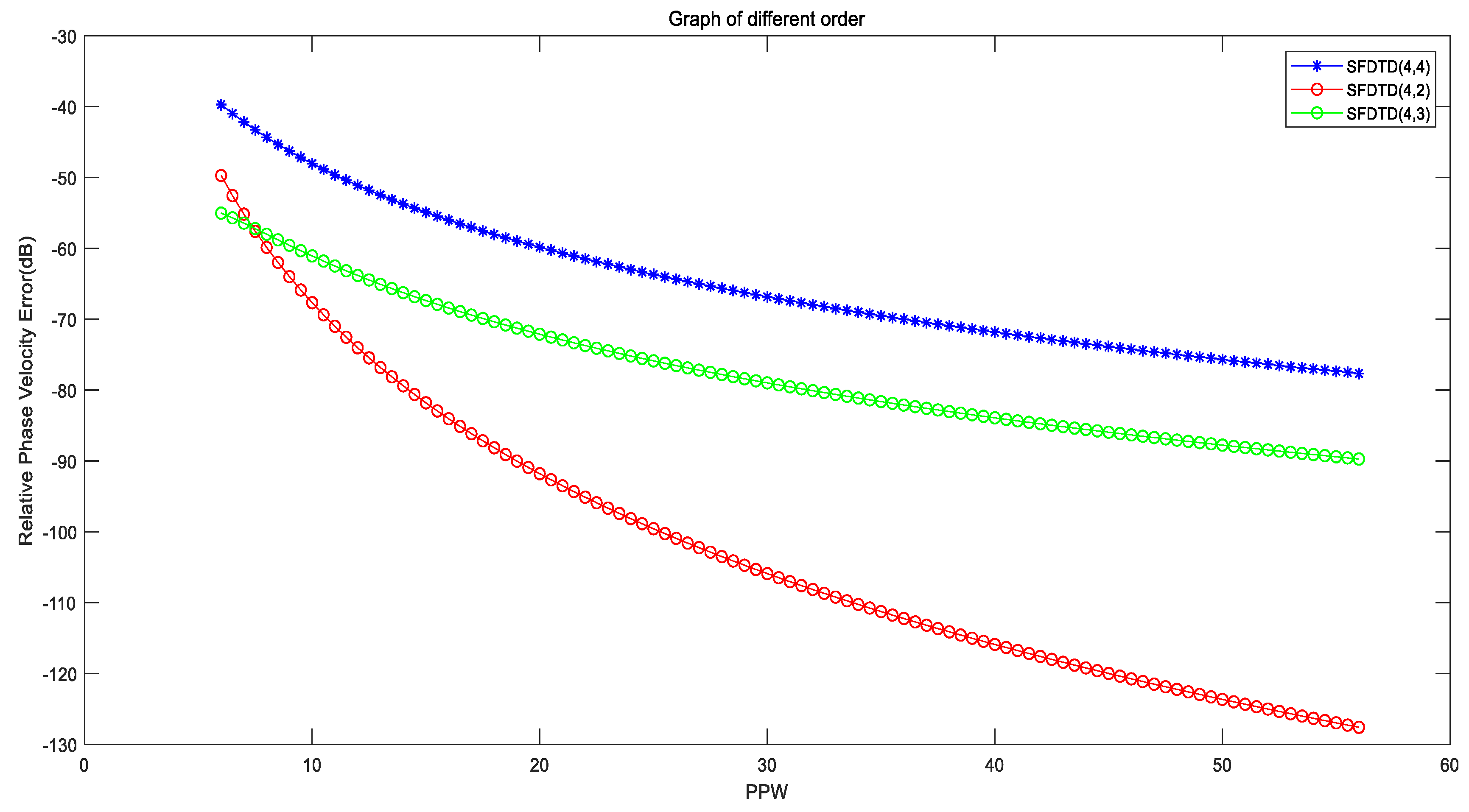
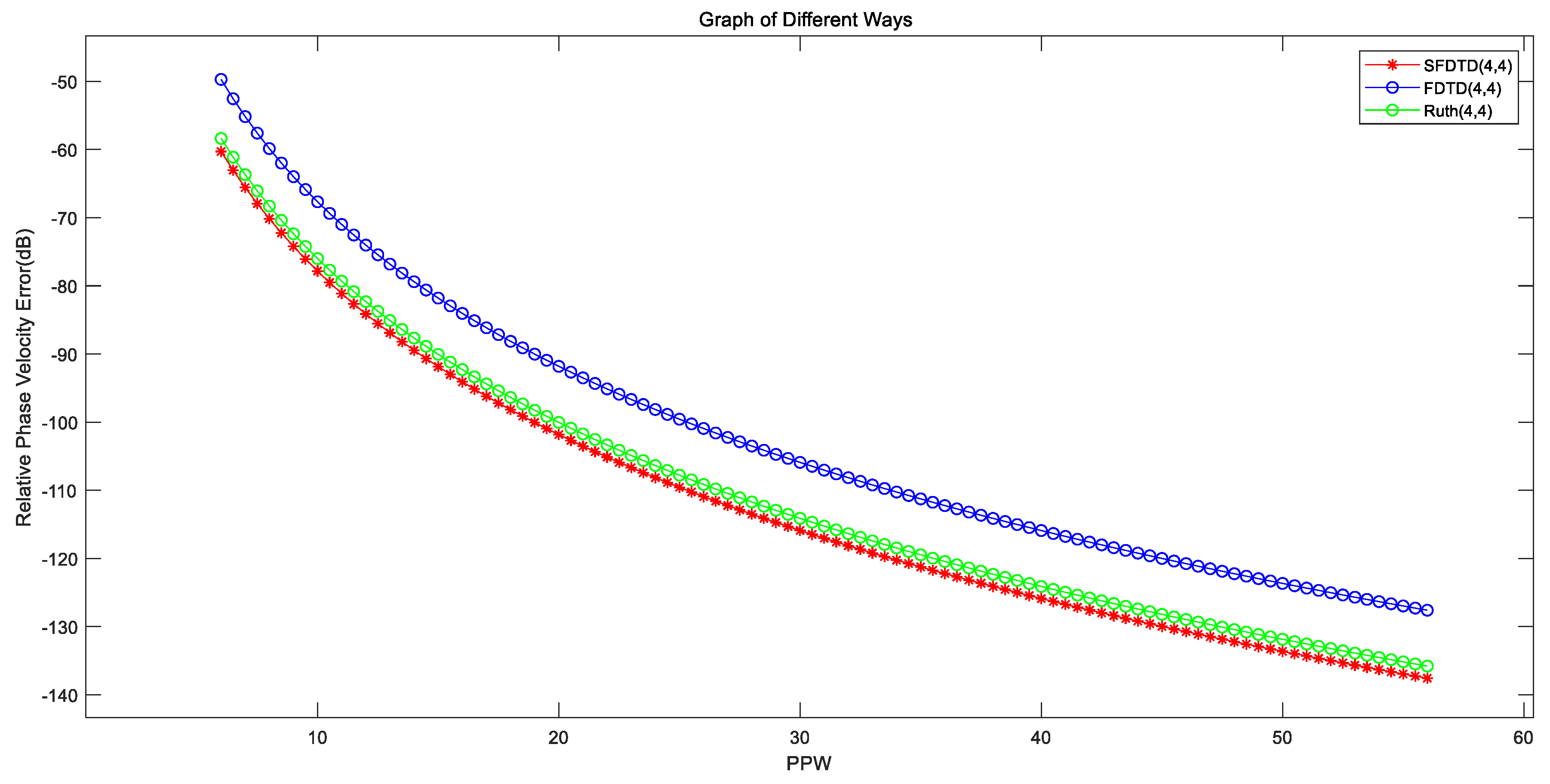
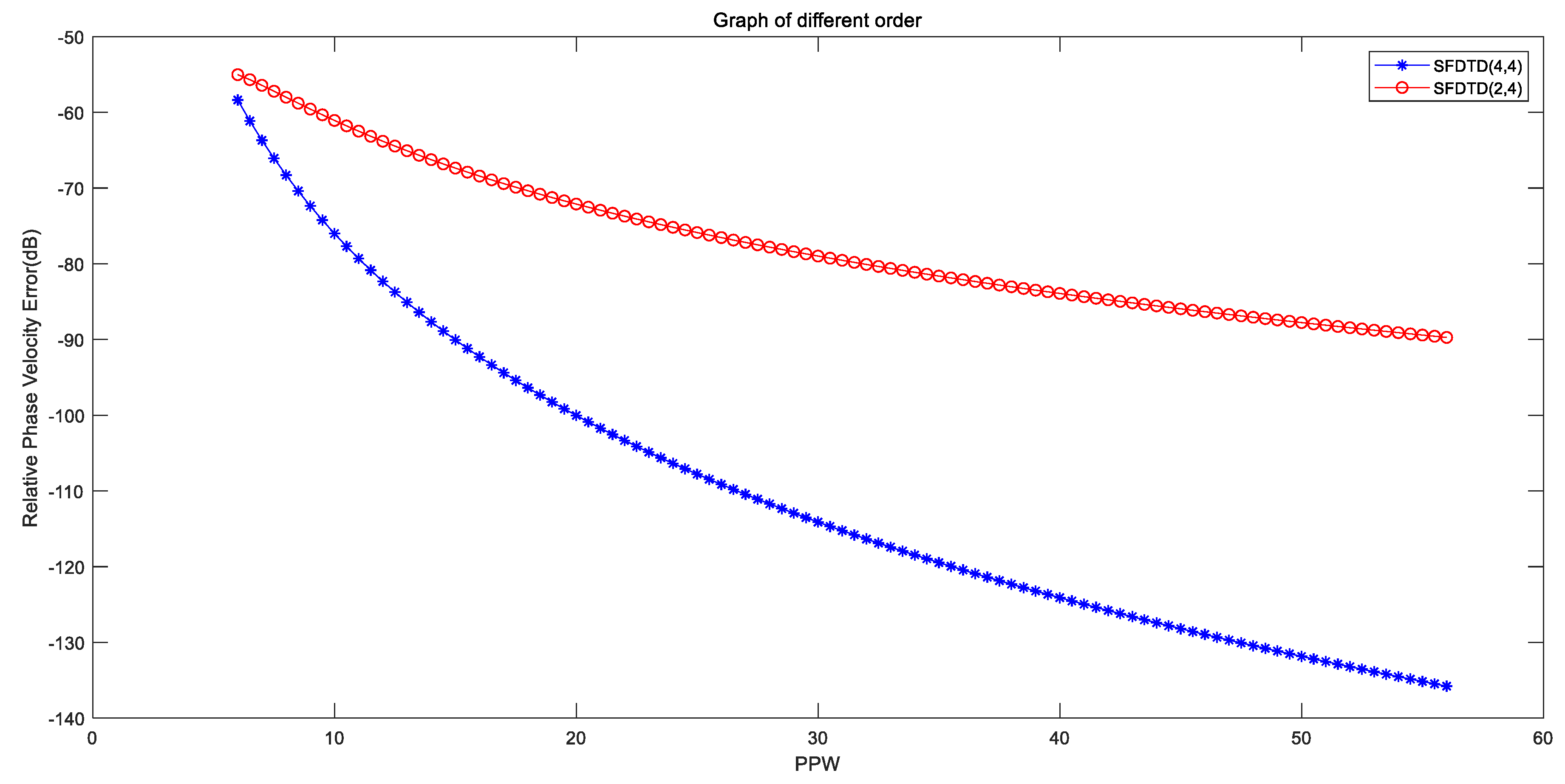
2.2. Comparison with Different Symplectic Operators

For the ordinary numerical analysis method, as the calculation progresses, the numerical solution obtained and the cumulative error of the Hamilton system will become larger and larger. SFDTD represents the Symplectic Finite-Difference Time-Domain. The symplectic algorithm based on the decomposition symplectic operator can not only obtain the exact value of the symplectic propagation coefficient, but also effectively reduce the dispersion error.

Table 1. Value of symplectic operator propagation coefficient. SFDTD, Symplectic Finite-Difference Time-Domain.

(c,d)	c	d
SFDTD (2,4)	$c_1=0.6891,$ $c_2=0.3207$	$d_1=-2.70309412,$ $d_2=-0.53652708,$ $d_3=2.37893931,$ $d_4=1.86068189$
SFDTD (4,2)	$c_1=0.3163393038,$ $c_2=-0.081630997,$ $c_3=0.53047572287179,$ $c_4=0.20367456$	$d_1=0.7432,$ $d_2=0.3021$
SFDTD (4,3)	$c_1=0.81431,$ $c_2=-0.31431,$ $c_3=-0.31431,$ $c_4=0.81431$	$d_1=-0.093769,$ $d_2=1.18653,$ $d_3=-0.093769$
SFDTD (4,4)	$c_1=0.2581,$ $c_2=1.3821,$ $c_3=-0.2403,$ $c_4=-0.5317$	$d_1=0.4311,$ $d_2=-0.0722,$ $d_3=0.1411,$ $d_4=0.5013$
Ruth (4,4)	$c_1=0.6756,$ $c_2=-0.1756,$ $c_3=-0.1756,$ $c_4=0.6756$	$d_1=1.3512,$ $d_2=-1.7024,$ $d_3=1.3512,$ $d_4=0$

gives the values of different symplectic operators. By comparing the second-order with different order symplectic operators, Figure 4 clearly shows that the dispersion error gradually increases with the increase of the order while keeping the series constant. In the same order, by comparing the symplectic operators of different series in Figure 5, it is also found that the higher the number of symplectic operators, the better the dispersion characteristics.

Comparing the dispersion error of different methods in Figure 6, we can clearly see that the imaginary operator that we have solved by pure mathematical derivation can achieve good dispersion characteristics.

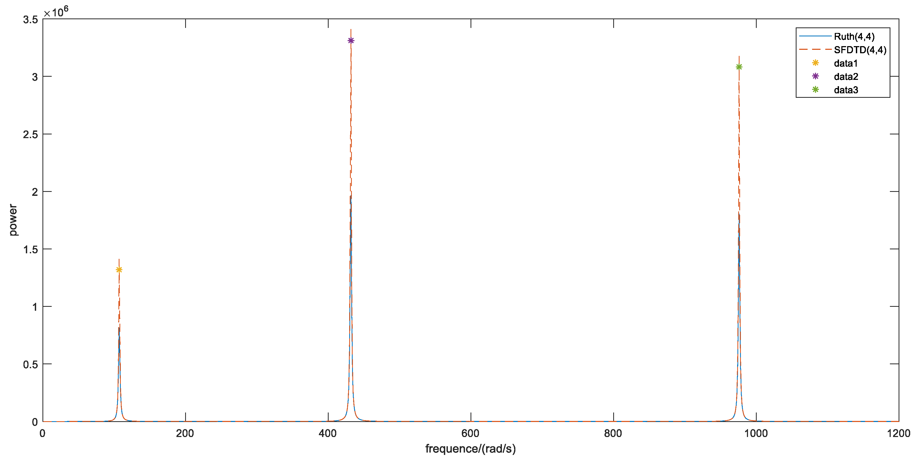
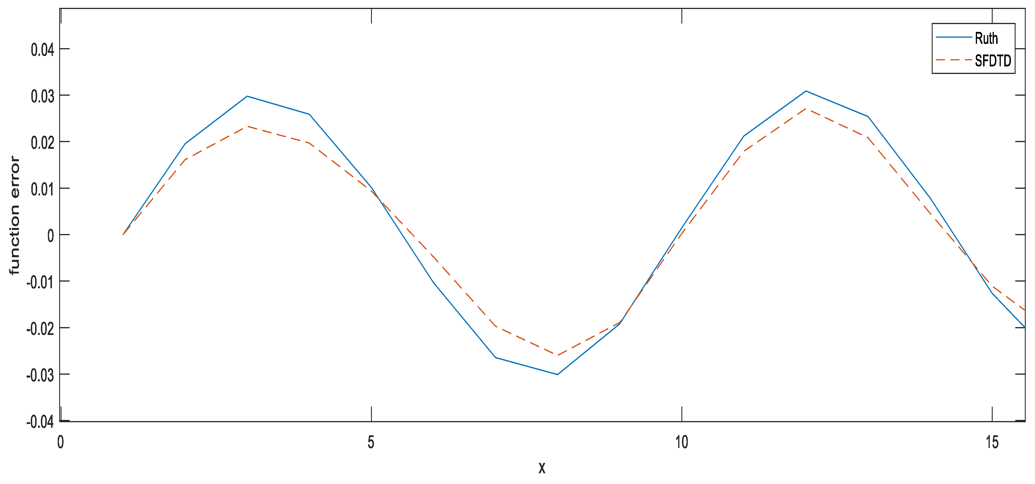
3. Application in the Intrinsic Problem of Nanodevices

In quantum mechanics, an infinitely deep square well is a potential well with a potential in the well of 0 and an infinite potential outside the well. The expression is [17].

$V\left(x\right)=\{\begin{array}{cc}0,& 0\le x\le a\\ \infty ,& else\end{array}$, a represents the length of the box, and x represents the position of the particle.

For the cube region, the eigen energy of the quantum well is $E_n=\frac{h^2{\pi }^2}{2m{a}^2}{n}^2,n=1,2,\dots$, the resonance frequency is ${\omega }_n=\frac{E_n}{h}=49.3928n^2,n=1,2,\dots$, the box size is $x\in \left[0,34\right]$, the space step is $\tau =1$, and the stability is $S_{\delta }=\frac{\tau h}{{\Delta }_x^{2}m}=0.1$, $N_{max}=41,000$. The energy distribution of the spectrum of the particle wave function in the box was shown in see Figure 7. We calculate the resonance frequency by using different symplectic operators respectively. For analysis and comparison, it can be clearly seen from Figure 8 that the error between the symplectic algorithm and the analytical solution obtained by theoretical calculation is smaller.

4. Conclusions

In view of the insufficiency of the dispersion error caused by simplification and many artificial assumptions such as symmetry and time reversibility in the process of solving traditional symplectic operators, we calculate different orders by solving the Hamilton equation with purely mathematical derivation. The new symplectic operators correspond to different series of numbers without making any assumptions and artificial simplifications, and reduce the dispersion error from the source. On the basis of comparing different symplectic operators such as (2,4), (4,2), (4,3), and (4,4), we have selected the fourth-order as the main research object. The fourth-order new symplectic operator is applied to the intrinsic problem of nanodevices to solve the one-dimensional Schrödinger equation. Comparing the symplectic operator method with the traditional FDTD method and Ruth’s method, the comparison of the energy distribution of the wave function spectrum calculated by these three methods and the real error value of the wave function at the center frequency fully proves that our method is feasible because of its higher precision and lower dispersion error. This method can also be widely used in other fields, and its dispersion characteristics require further testing.

References

1. Fu, M.; Liang, H. An improved precise Runge-Kutta integration. Acta Sci. Nat. Univ. Sunyatseni 2009, 5, 1–5. [Google Scholar]
2. Prokopidis, K.P.; Zografopoulos, D.C. One-step leapfrog ADI-FDTD method using the complex-conjugate pole-residue Pairs dispersion model. IEEE Microw. Wirel. Compon. Lett. 2018, 28, 1068–1070. [Google Scholar] [CrossRef]
3. Feng, K.; Qin, M. Symplectic Geometry Algorithm of Hamilton System; Zhejiang Science and Technology Press: Zhejiang, China, 2003. [Google Scholar]
4. Ruth, R.D. A Canonical integration technique. IEEE Trans. Nucl. Sci. 1983, 30, 2669–2671. [Google Scholar] [CrossRef]
5. Iwatsu, R. Two new solutions to the third-order symplectic integration method. Phys. Lett. A 2009, 373, 3056–3060. [Google Scholar] [CrossRef]
6. Cui, J.; Hong, J.; Liu, Z.; Zhou, W. Stochastic symplectic and multi-symplectic methods for nonlinear Schrödinger equation with white noise dispersion. J. Comput. Phys. 2017, 342, 267–285. [Google Scholar] [CrossRef]
7. Milstein, G.N.; Repin, Y.M.; Tretyakov, M.V. Numerical methods for stochastic systems preserving symplectic structure. SIAM J. Numer. Anal. 2002, 40, 1583–1604. [Google Scholar] [CrossRef]
8. Mcmahon, J.M.; Gray, S.K.; Schatz, G.C. A discrete action principle for electrodynamics and the construction of explicit symplectic integrators for linear, non-dispersive media. J. Comput. Phys. 2009, 228, 3421–3432. [Google Scholar] [CrossRef]
9. Xiao, J.; Qin, H.; Morrison, P.J.; Liu, J.; Yu, Z.; Zhang, R.; He, Y. Explicit high-order noncanonical symplectic algorithms for ideal two-fluid systems. Phys. Plasmas 2016, 23, 112107. [Google Scholar] [CrossRef]
10. Wen, Y.Y. Symplectic Algorithm and Its Application in Electromagnetic Field Equations. J. Microw. 1999, 1, 68–79. [Google Scholar]
11. Qing, G.H.; Tian, J. Highly accurate symplectic element based on two variational principles. Acta Mech. Sin. 2018, 34, 151–161. [Google Scholar] [CrossRef]
12. Liang, L.N.; Yan, B. Study on the Schrödinger equation of hydrogen molecular ion by linear variational method. Chem. Manag. 2017, 36, 27–28. [Google Scholar]
13. Feng, L.Q. Characteristics of He~+ high-order radiation harmonics under butterfly metal nanostructures. Chin. J. Quantum Electron. 2018, 35, 479–485. [Google Scholar]
14. Cheng, C.; Wang, G.D.; Cheng, Y.Y. Effect of surface polarization on the band gap and absorption peak wavelength of quantum dots at room temperature. Acta Phys. Sin. 2017, 66, 238–245. [Google Scholar]
15. Liu, J.X.; Feng, S.M.; Gu, L.H.; Lei, G.; Yan, X.M. Relationship between Surface Barrier and Surface Energy Level and Experimental Research. Shanghai Aerosp. 2017, 34, 105–109. [Google Scholar]
16. Magri, F. A simple model of the integrable Hamiltonian equation. J. Math. Phys. 1978, 19, 1156–1162. [Google Scholar] [CrossRef]
17. Thompson, L.D. One-dimensional infinite square well potential. Phys. Educ. 1984, 19, 167. [Google Scholar] [CrossRef]
Figure 1. In the second-order, different symplectic operators are represented in the image with d1. It can be found that different symplectic operators change greatly with the value of d1, thus affecting the whole algorithm.
Symmetry 11 01383 g001
Figure 2. The second-order symplectic operator error function image, we can find from the image that the error function fluctuates with the value of d1 and there is a minimum in a certain range.
Symmetry 11 01383 g002
Figure 3. The variation of the symplectic operators with the d1 in the third-order symplectic algorithm.
Symmetry 11 01383 g003
Figure 4. Comparing the symplectic algorithms of different orders, it can be clearly seen that the fourth-order symplectic algorithm has the best dispersion characteristics.
Symmetry 11 01383 g004
Figure 5. Comparing the different levels of the symplectic algorithm, it can be clearly seen that the higher the number of stages, the better the dispersion characteristics of the symplectic algorithm.
Symmetry 11 01383 g005
Figure 6. By Comparing the symplectic algorithm of the same order number obtained by the current research with the symplectic algorithm obtained by Ruth [4], we can see that our method is significantly better than the traditional method.
Symmetry 11 01383 g006
Figure 7. The energy distribution of the spectrum of the particle wave function in the box.
Symmetry 11 01383 g007
Figure 8. Real error comparison.
Symmetry 11 01383 g008