Energy Modeling and Experimental Validation of Four-Wheel Mecanum Mobile Robots for Energy-Optimal Motion Control

Abstract

Four-wheel Mecanum mobile robots (FWMRs) are widely used in transportation because of their omnidirectional mobility. However, the FWMR trades off energy efficiency for flexibility. To efficiently predict the energy consumption of the robot movement processes, this paper proposes a power consumption model for the omnidirectional movement of an FWMR. A power consumption model is of great significance for reducing the power consumption, motion control, and path planning of robots. However, FWMRs are highly maneuverable, meaning their control is complicated and their energy modeling is extremely complex. The speed, distance, path, and power consumption of the robot can vary greatly depending on the control method. This energy model was mathematically implemented in MATLAB and validated by our laboratory’s Mecanum wheel robot. The prediction accuracy of the model was over 95% through simulation and experimental verification.

1. Introduction

In recent years, with the extensive use of mobile robots, more and more researchers have focused on reducing the energy consumption of these robots. Energy efficiency is a key constraint on robot performance. Because mobile robots are generally driven by batteries, reducing their energy consumption can increase the use time of robots, reduce the number of battery charges, and reduce production costs. Many works have appeared presenting novel mechanical designs, control strategies, or trajectory planning algorithms for improved energy efficiency [1]. The energy model can output an actual estimation of the energy needed, which can be useful in practical applications [2,3] such as mission energy prediction [4], scheduling [5], and the generation of cheaper paths and trajectories [6].

Four-wheel Mecanum mobile robots (FWMRs) do not need to change their body postures while in omnidirectional motion, and they can rotate around their center at the same time. The omnidirectional movement is thus made as a result of the different velocities of the Mecanum wheels [7]. Because of the omnidirectional mobility of FWMRs, their control and motion modes are also complicated. When an FWMR’s path planning and scheduling are made, the energy consumption of different paths and different control modes along the paths is also different. Consequently, FWMR energy consumption models are very complex.

To get an accurate energy consumption model, the power consumption characteristics of the omnidirectional movement process of robots are studied in this paper. When analyzing the power consumption of the FMWR, we first modeled the speed of the robot, and then divided the power consumption of the robot into three systems (i.e., the control system, the sensing system, and the motion system), which were analyzed separately for power consumption. The path is an important parameter of energy consumption, but considering only the energy consumption model of the path would be incomplete because different control methods lead to different energy consumption models. In the modeling, we focused on the analysis of the model of motion energy consumption, adding parameters so that we could analyze the energy consumption under different control methods.

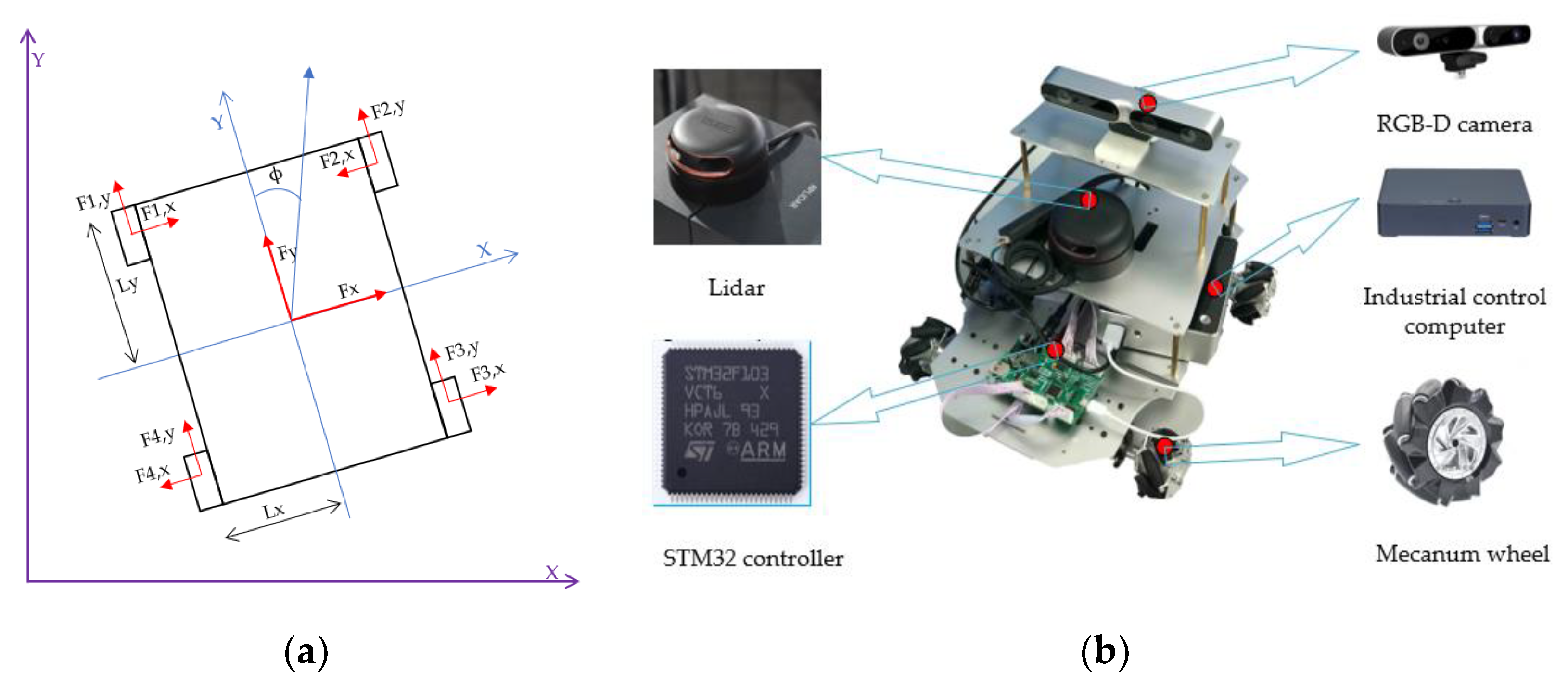
As shown in Figure 1, the common architecture of mobile robots usually consists of batteries, motors, motor drivers, controllers, sensors, and communication devices.

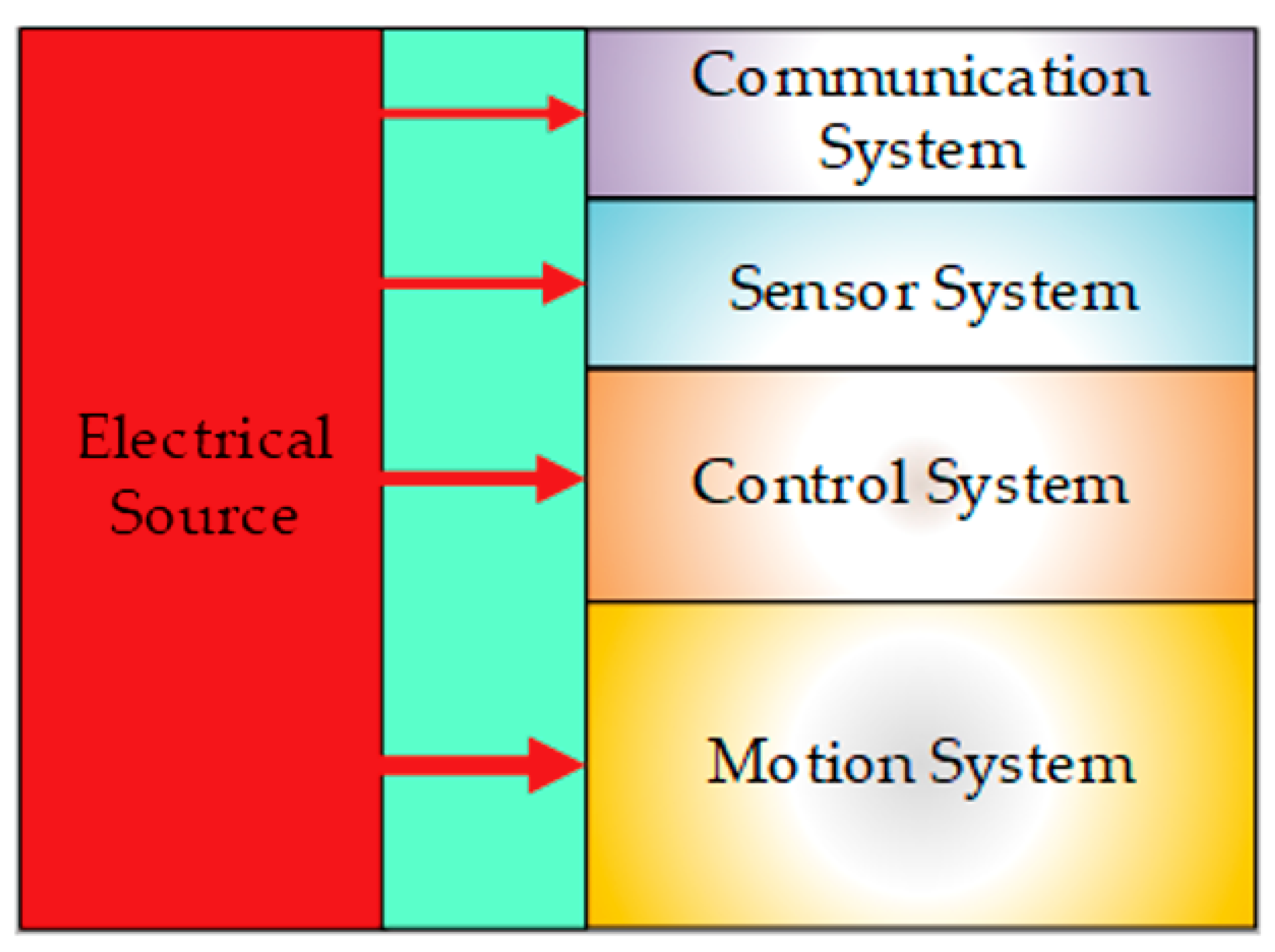
Energy is consumed primarily by the functions of the FWMR’s motors, sensors, microcontroller, and embedded computer [8,9]. The sources of energy consumption can be divided into the motion system, the control system, the sensor system, and the communication system. The power consumption of the motion system is the largest of the four systems [2,10], as shown in Figure 2.

The energy consumption model was built based on a comprehensive understanding of the energy flow of the mobile robot [11,12]. A complete energy model needs to cover all the energy consumption associated with robot control and motion. In this way, it is possible to obtain accurate energy consumption in the cases of different control methods and motion modes of the robot. Energy-saving motion control is an important research issue in mobile robots [13]. Because of the extraordinary mobility of FWMRs, minimum-energy trajectory is also an important research issue [14]. The corresponding energy consumption is different when traveling through different trajectories under different control methods. Despite many studies on obstacle avoidance and optimal path planning [15,16], it must be pointed out that the optimal path is not necessarily the path with the least energy consumption for FWMRs. In general, shorter paths will result in reduced energy consumption. However, the power consumption of an FWMR in the process of acceleration is very high. If the robot is accelerated and decelerated frequently [2], the energy consumption will greatly increase.

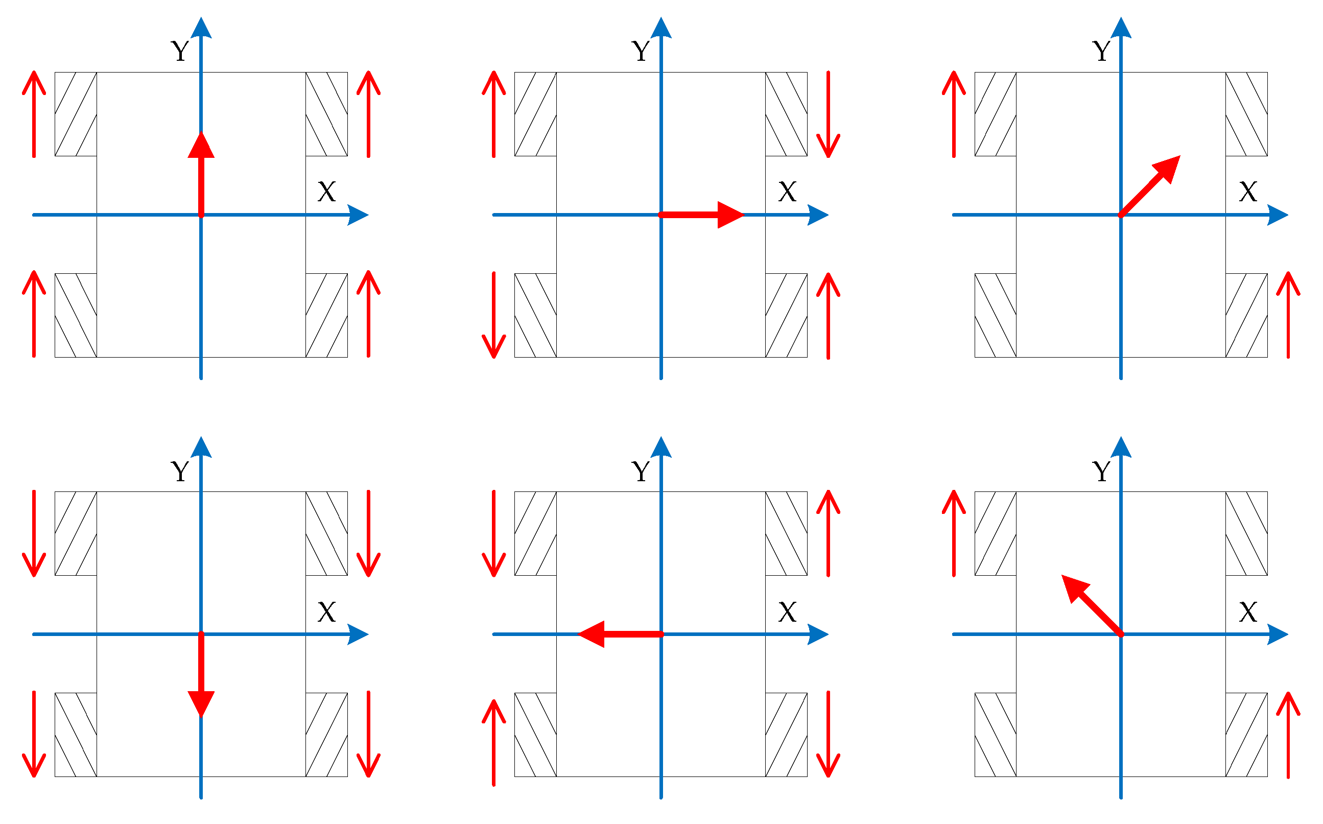
The energy consumption of the moving part is the largest, so the motion plan is a very important research direction [17]. Since they move using four independent motor actuators, FWMRs can move in arbitrary directions with arbitrary orientations [18], which make the motion planning in complicated and narrow places easier to control [19,20]. An FWMR moves in different directions [21], and its energy consumption changes because of the different friction offsets. Due to its symmetrical structure, an FWMR has the same friction offset when the wheel rotates at the same speed.

The direction of the driving wheel and the direction of the robot’s motion are shown in Figure 3. The robot is completely symmetrical in kinematics during the omnidirectional movement, and its direction of motion and friction offset are also symmetrical. Therefore, in the process of power analysis, we only need to analyze the power consumption within 90°.

The rest of this paper is structured as follows. We first discuss the energy consumption modeling of FWMR in Section 2. In Section 3, we evaluate energy consumption and results are analyzed. Conclusions and future works are discussed in Section 4.

2. FWMR Energy Consumption Modeling

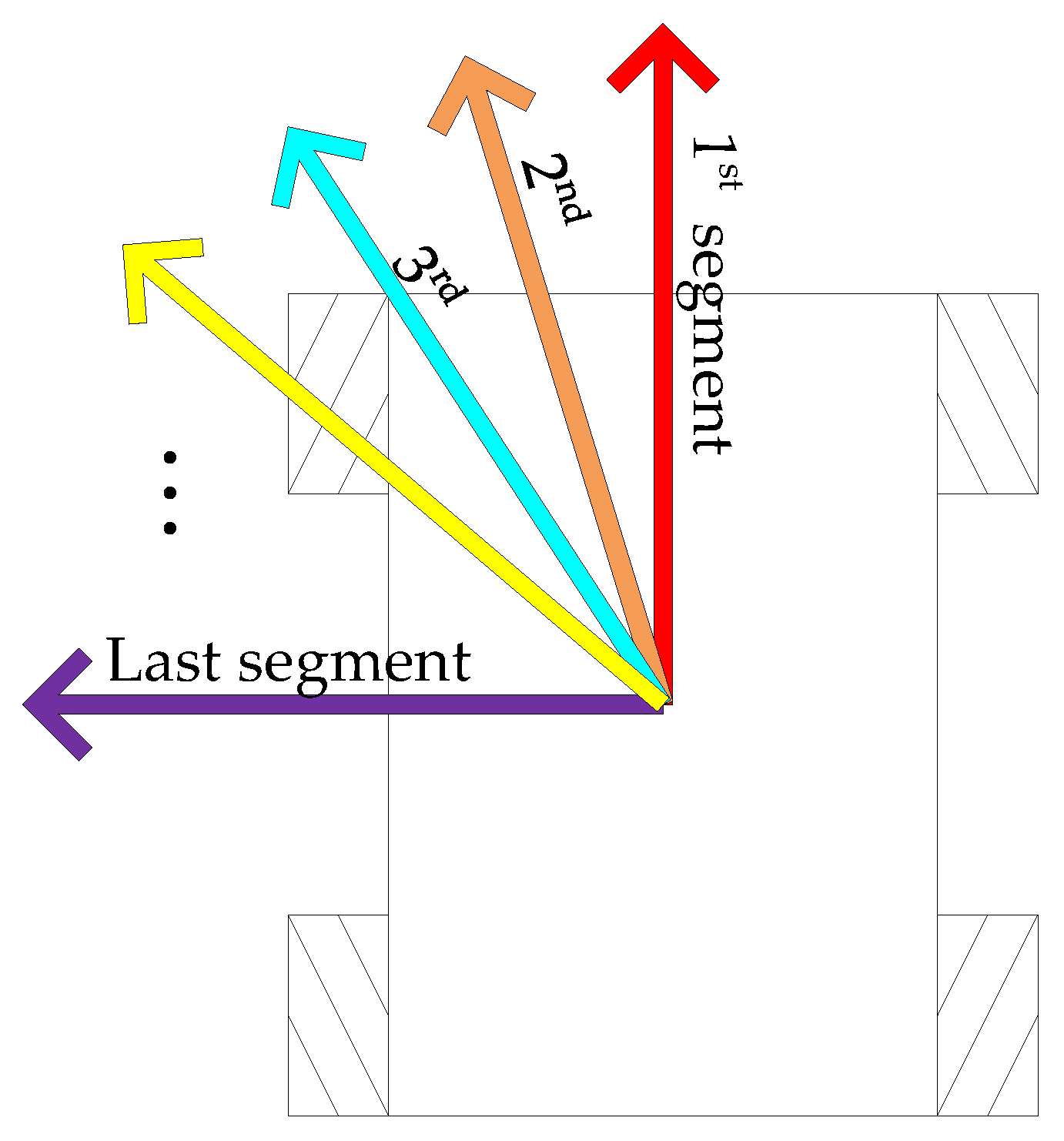
FWMRs are structurally symmetrical and holonomic [22], which enables them to move in any direction within 360°. As shown in Figure 4, within a 90° range, the FWMR can move in a straight line at any angle. Because the friction offset between the wheels is inconsistent when it moves in different directions, the power consumption of the robot is also different.

In order to ensure the accuracy of the robot’s measurement during the motion, we confined the motion of the robot to within 90°. The method we used during the motion was performed every 3° so that we could guarantee that we had enough examples.

The power consumption of the FWMR was directly related to its speed and acceleration. To accurately analyze the power consumption of the FWMR during operation, we first modeled the speed of the robot during the running process. This method of speed modeling required us to read the instantaneous speed of the vehicle through the encoder, and the instantaneous velocity was then mathematically modeled and analyzed.

In order to ensure the accuracy of the robot power analysis, the proportional–integral–derivative (PID) control method [23] was used to control the speed of the robot in the omnidirectional movement process. In order to control the FWMR’s movement along the preset path and direction, it was necessary to control the speed of all four wheels accurately. Due to the mechanical structure, sensors, motors, and other errors, it was impossible to get an accurate control formula, so the PID control was very suitable to our study.

The speed curve of the robot during the omnidirectional movement is shown in Figure 5. The speed and the starting mode of the robot are specified, having used the PID control method to ensure that the robot would strictly follow the speed curve set by us, thus ensuring that the robot’s speed would not affect its power consumption.

Figure 5. illustrates that the speed of the robot changed very sharply. In about 0.3 s, the FMWR reached the maximum speed we set (1 m/s), and it maintained this speed thereafter.

Because the robot was powered by a lithium battery, it followed the rules in terms of power consumption [1]:

$$E_{robot}={\displaystyle \int P_{source}}dt.$$

(1)

$E_{robot}$ is the power consumption of the robot, $P_{source}$ is the power of the lithium battery. In order to carry out a complete analysis of the power consumption of the FWMR’s omnidirectional movement, we divided the power consumption of the robot into four systems. In this article, the power consumption of the four systems was separately analyzed to learn the power consumption characteristics of the omnidirectional movement.

$$E_{robot}=E_{motion}+E_{control}+E_{sensor}+E_{communication},$$

(2)

where $E_{motion}$ is the power consumption of the robot’s motion system, $E_{control}$ is the power consumption of the robot control system, $E_{sensor}$ is the power consumption of the robot sensing system, and $E_{communication}$ is the power consumed by the robot’s communication system.

The research in this paper served mainly to model the power consumption of the robot in the omnidirectional movement process. In this process, the main change is in the power consumption of the robot’s motion system. Therefore, that was our focus. For the control systems, sensing systems, and communication systems, we performed only a qualitative analysis. We performed a detailed analysis of the motion system.

2.1. Energy Consumption Modeling of the Motion System

The power consumption of the robotic motion system was divided into five parts based on the characteristics of the motor [24]:

$$E_{motion}={\displaystyle \int P_{motion}dt=E_e+E_f+E_c+E_h+E_k},$$

(3)

where $E_{motion}$ is the energy consumed by the robot’s motion system, $P_{motion}$ is the power consumption of the robot’s motion system, $E_c$ is the work of the frictional forces that cancel each other out during the FWMR movement, $E_f$ is the work done to overcome the frictional resistance during the movement, $E_e$ is the mechanical dissipation during the movement and the dissipation of the motor itself, $E_h$ is the power consumption dissipated in the form of thermal energy, and $E_k$ 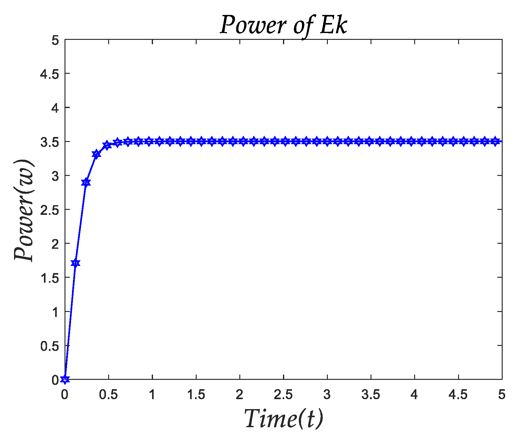is the increase of the kinetic energy of the robot during its movement.

Figure 6 represents the kinetic energy of the robot. The kinetic energy of the robot corresponded to the square of the speed of the robot. |Therefore, we expressed the kinetic energy of the robot as:

$$E_k=M{v}^2/2.$$

(4)

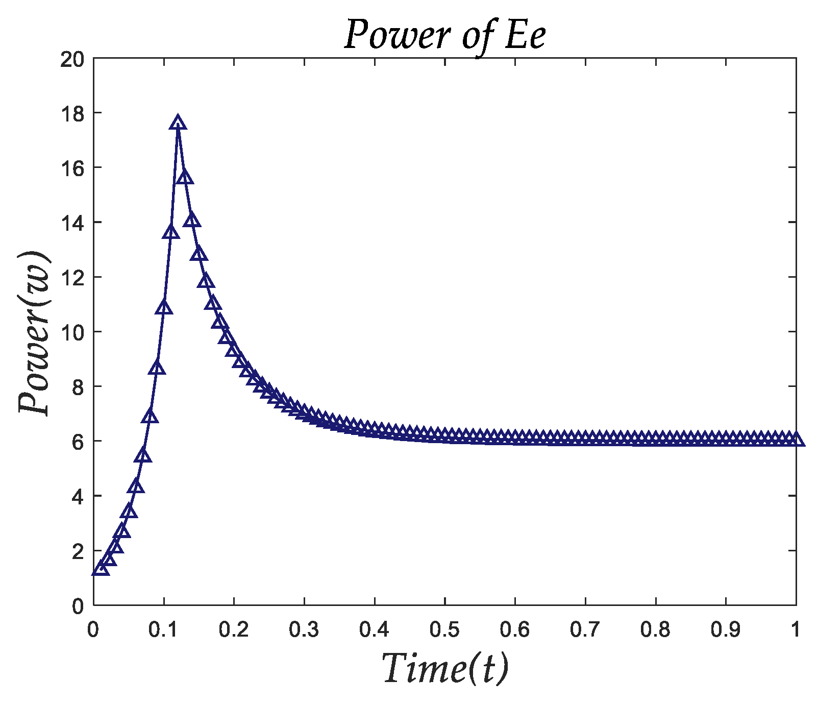
The mechanical dissipation of the robot during its movement is mainly related to the speed and quality of the robot, and the dissipation of the motor is mainly related to the speed of each wheel of the robot and the movement time of the robot. Therefore, $E_e$ can be expressed as:

$$E_e={\displaystyle \int \left(MgR/{\left(v-v_0\right)}^2{v}^{1/2}+{\left(\frac{1}{t}\right)}^{\kappa }+{\displaystyle \sum _{i=1}^{4}Mg{v}_i^2}\right)}dt,$$

(5)

where $M$ is the mass of the robot and $v$ is the speed of the robot. This part of the energy is the main energy consumed by the robot’s motion system. Figure 7 shows the power changes of $E_e$.

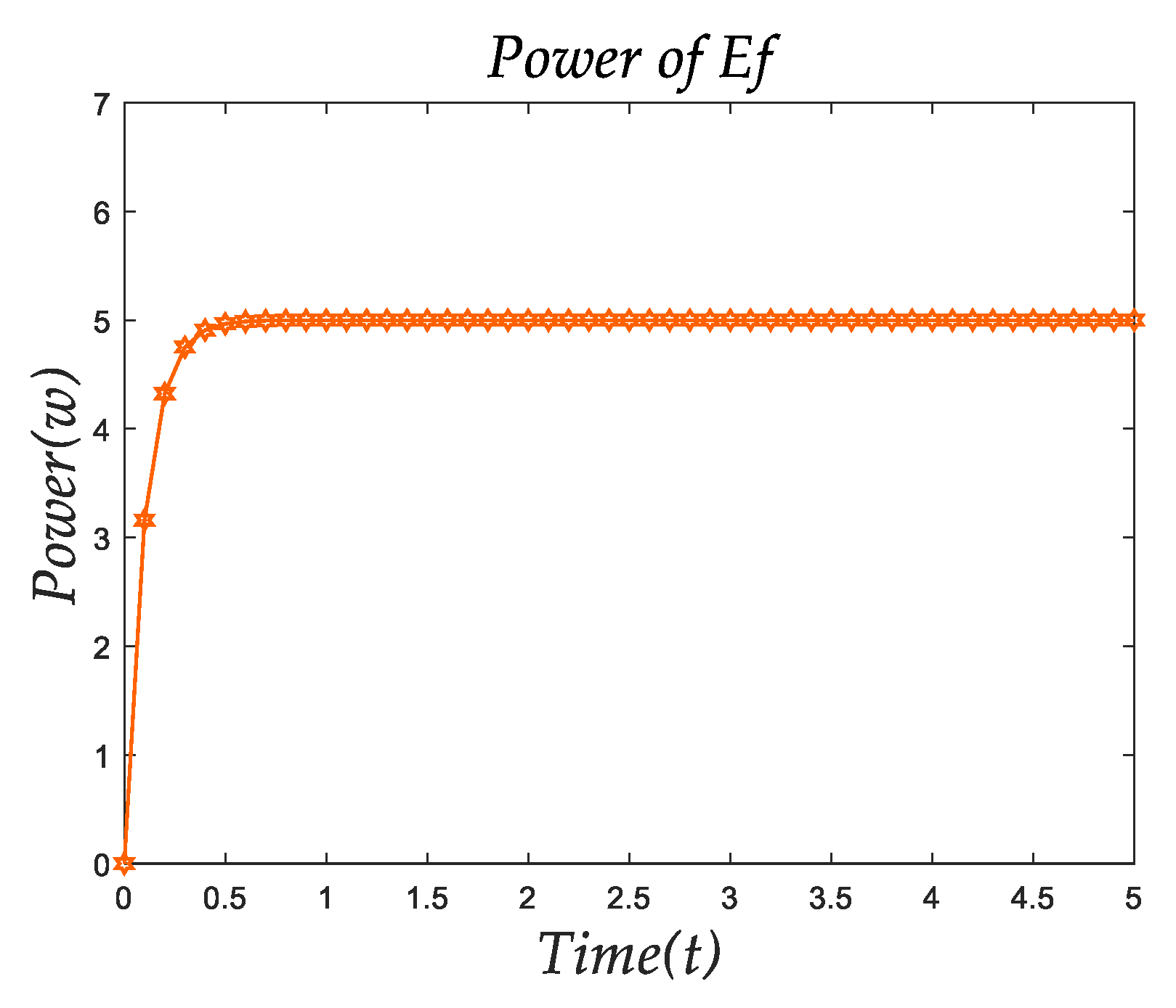
The energy of the friction loss of the robot is mainly related to the speed of the robot and the friction coefficient of the robot, because the friction of the Mecanum wheel robot exhibits not only sliding friction but also rolling friction. So, $E_f$ can be expressed as:

$$E_f={\displaystyle \int \left(\left({\mu }_R{\displaystyle \sum _{i=1}^4{v}_i}\right)+\left({\mu }_s{\displaystyle \sum _{i=1}^4{v_i}^{\prime }}\right)\right)}dt,$$

(6)

where $M$ is the mass of the robot, $v$ is the speed of the robot, and $v_i$ is the speed of each wheel of the robot. Figure 8 shows the power changes of $E_f$.

Table 1. Mecanum wheel constants as measured through different wheels.

	Front	Back	Mean
Motor 1 (Left motor)
${\mu }_R$	0.0025	0.0029	0.0027
${\mu }_s$	1.7255	1.7259	1.7257
Motor 2 (Right motor)
${\mu }_R$	0.0023	0.0025	0.0024
${\mu }_s$	1.7252	1.7254	1.7253

shows the parameters of the Mecanum wheel. Because the degrees of wear of the four Mecanum wheels were different, their parameters differed.

$\mu$ is the friction coefficient of the robot, which is mainly related to the robot’s center of gravity. Therefore, the robot’s friction parameter can be expressed as:

$$\mu =2L_R/\left(L_R+L_S\right)*{\mu }_s+2L_S/\left(L_R-L_S\right)*{\mu }_R.$$

(7)

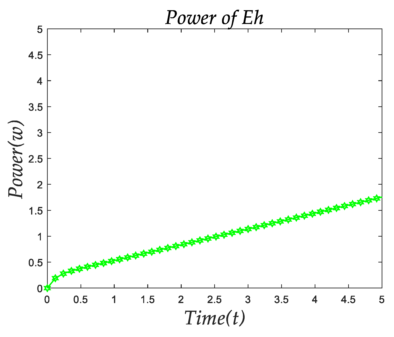
The thermal energy dissipation of the robot is mainly related to the thermal energy dissipation of the motor and the heat dissipation of the control board. The thermal energy dissipation of the robot is mainly related to the speed of the robot and its running time. Therefore, $E_h$ can be expressed as:

$$E_h={\displaystyle \int \left(\beta \left({{\displaystyle \sum _{i=1}^4{v}_i}}^2\right)+\epsilon {\displaystyle \sum _{i=1}^n{v}_i}+\lambda t^2+\eta t\right)}dt.$$

(8)

In Equation (8) and are the velocity parameters, is the time parameter, is the speed constant. is directly related to the temperature of the motor and the speed of the motor, so can be expressed as:

$$\beta =k_{10}{\left(1+{\alpha }_R\left(T-T_0\right)\right)}^2{\left(1+{\alpha }_M\left(v_{\max }-v\right)\right)}^{-2}+k_{20}{\left(1+{\alpha }_M\left(v_{\max }+v\right)\right)}^{-4},$$

(9)

where $k_{10}$ and $k_{20}$ are proportionality constants, and the proportionality constants are different depending on the characteristics of each motor. $\epsilon$ is the speed parameter, which is directly related to the speed of each wheel and the initial temperature of the motor and the current temperature, so $\epsilon$ can be expressed as:

$$\epsilon =k_{20}\left(2+{\alpha }_M\left({\displaystyle \sum _{i=1}^4{v}_i^2}\right)\right)+k_{10}{\left(2+{\alpha }_R\left(T-T_0\right)\right)}^2.$$

(10)

$\lambda$ is the time parameter, which is mainly related to the temperature of the robot, so it can be expressed as:

$$\lambda \left(T\right)=k_{10}\left(1+{\alpha }_R{\left(T-T_0\right)}^{-1}\right)+k_{20}\left(2+{\alpha }_R{\left(T-T_0\right)}^{-2}\right).$$

(11)

The power consumed by the robot in the form of heat is shown in Figure 9, where the energy consumed by the robot in the form of thermal energy increased with the increase in running time, but in general this amount of energy was still very low.

$$E_c={\displaystyle \int \left(\mu Mg{L}_y\left({\displaystyle \sum _{i=1}^4{v}_i}\right)\sin \left(\varphi -\frac{\pi }{4}\right)+\mu Mg{L}_{\mathrm{y}}/L_x\left({\displaystyle \sum _{i=1}^4{v}_i^2}\right)\right)}dt$$

(12)

The Mecanum wheel robot can achieve omnidirectional motion by way of the Mecanum wheels, which produce the resultant force in any direction during the movement. Power consumption is generated between the wheels of the robot during movement, which is often cancelled out by friction. The offset of power consumption changes is shown in Figure 10. It can be seen from Figure 10 that the power loss of the robot due to the frictional forces canceling each other out was roughly equal to the change of the speed of the robot, because the energy consumed by the robot due to friction is directly related to the robot’s angle of motion and speed.

Table 2. Motor constants as measured through different wheels.

	Front	Back	Mean
Motor 1 (Left motor)
$k_{10}$	0.0025	0.0029	0.0027
$k_{20}$	1.7255	1.7259	1.7257
Motor 2 (Right motor)
$k_{10}$	0.0023	0.0025	0.0024
$k_{20}$	1.7252	1.7254	1.7253

shows the motor constants as measured through different wheels. The motor constants are different for different motors. Here are the motor constants using the Mecanum wheels in this study.

Table 3. Modeled and actual values of motion system power consumption.

Time	Speed (m/s)	Modeled Motion System Power (W)	Measurement Power (W)
0	0	0	0
0.1	0.3	20.12	21.12
0.2	0.5	38.12	38.52
0.3	0.7	22.12	22.23
0.4	0.9	21.39	21.52
0.5	0.99	21.35	21.32
0.6	1.0	21.56	21.23
0.7	1.0	21.25	21.23
0.8	1.0	22.05	21.54
0.9	1.0	21.52	21.23
1.0	1.0	21.32	22.52
1.1	1.0	21.02	21.03
1.2	1.0	22.03	21.12
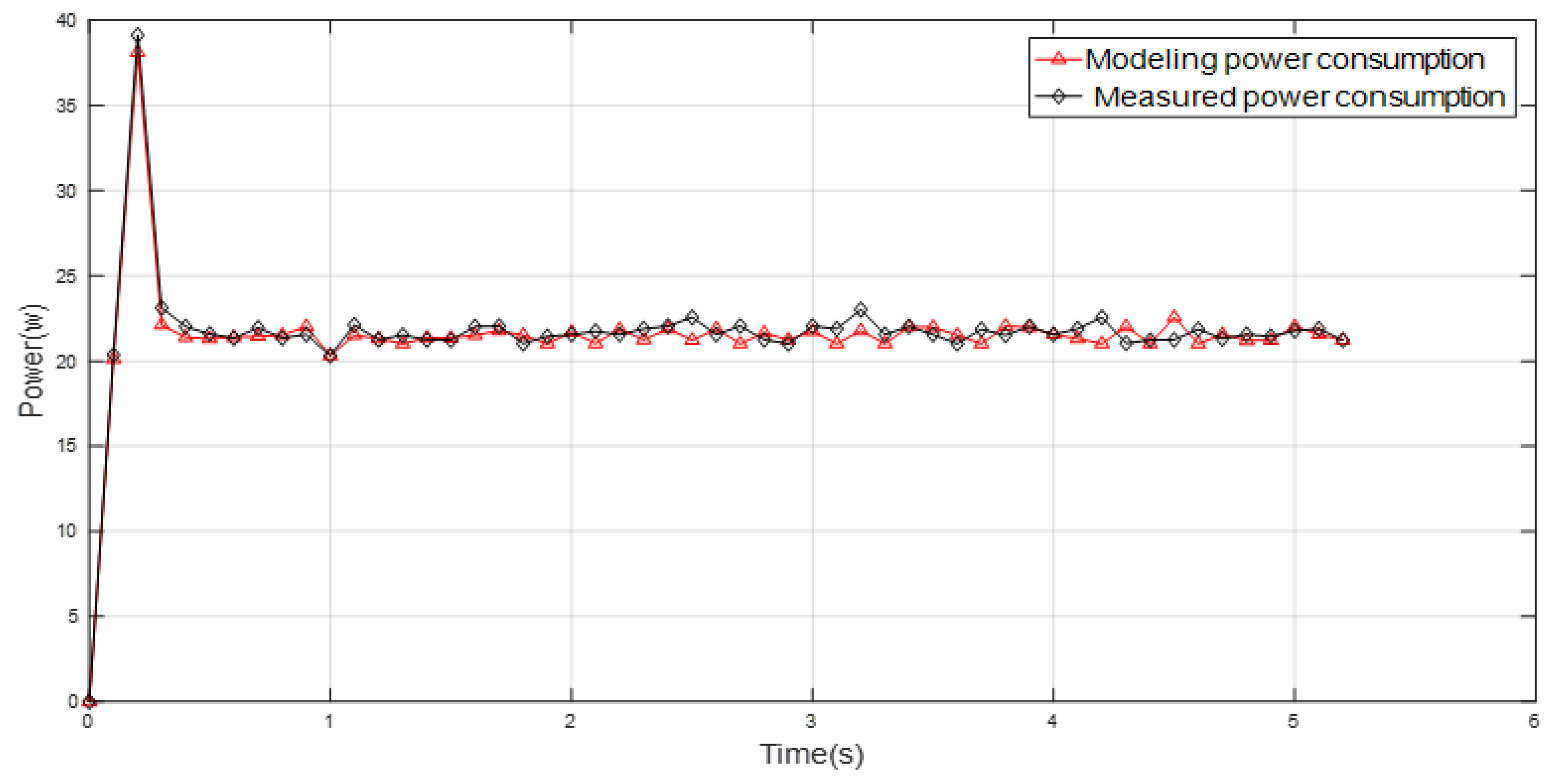
1.3	1.0	21.52	21.23

shows the comparison between the modeled and the actual values of the robot’s motion system.

Figure 11 shows the comparison between the modeled and measured power consumption. The accuracy of the robot motion system modeling was over 95%, and the robot’s power consumption during the motion was very good.

2.2. Energy Consumption Modeling of the Control System

The power consumption of the control system depends on the power consumption of the control circuit boards [25], which is related to the robot’s running state. The power consumption of the robot control system is mainly related to the speed change of the robot, and has a strong relationship with the robot’s movement angle. Because the movement of the robot at different angles is different for each wheel, the acceleration signal sent by the robot’s control system is also different. Therefore, the power consumption of the robot’s control system has a lot to do with the robot’s motion angle.

$$E_{control}={\displaystyle \int \left(Mg\left(L_x+L_y\right)/v*\cos \left(\varphi -\pi /4\right)+Mg{L}_y/\left(L_x*v\right)\right)}dt$$

(13)

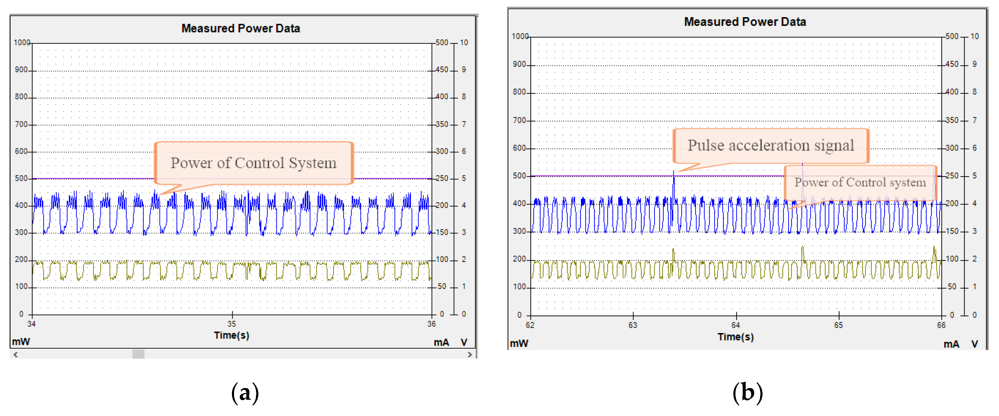
The power consumption of controller board was measured using an AAA10F power monitor (Monsoon Solutions). The measured value of the robot’s control system is shown in Figure 12. The robot had obvious pulses during acceleration and deceleration. In this process, the fluctuation of the robot’s control system became very dense. The power consumption of the robot increased significantly during this process.

From Figure 12a,b, we can see that the power consumption of the robot control system was related to the change of the robot’s motion state. During the robot’s motion, the acceleration value of the robot had a direct relationship with the power consumption of the robot control system. During the acceleration and deceleration of the robot, the robot’s control system needs to emit acceleration or deceleration pulses, which increases the robot’s power consumption.

2.3. Energy Consumption Modeling of the Sensor System

The power consumption of the sensing system is mainly related to the speed of the robot. The faster the robot moves, the greater the required sensitivity and operating speed of the sensing system. This results in an increase in the power consumption of the robot’s sensing system. The increase was great, so the power consumption of the robot’s sensing system was directly related to the speed of the robot [26].

Because the power consumption of the robot’s sensing system was still very stable relative to the motion system and the control system, only the power consumption of the robot’s sensing system was qualitatively analyzed, and no quantitative analysis was performed.

2.4. Energy Consumption Modeling of the Communication System

The power consumption of the robot’s sensing system is not related to the robot’s motion speed and motion direction. The power consumption of the robot communication system was very stable, but the robot’s communication system of the robot ran the longest. The robot’s communication system also needs to communicate in real time during the movement to ensure the normal communication between the robot and the external environment. Therefore, the power consumption of the robot’s communication system cannot be ignored.

3. Energy Consumption Evaluation and Result Analysis

In order to get a complete energy consumption model of the motion system, it was necessary to formulate the energy consumption under various motion conditions by applying the trajectory’s translational and rotational velocity profiles to it.

We needed to ensure that the speed of the robot remained the same during the experiment, so we set the maximum speed of the robot during the experiment. During the operation, we set the maximum speed of the robot to 1 m/s and moved the robot omnidirectionally. In the omnidirectional movement process, the speed of the robot changed as shown in

Table 4. Modeled and measured values of robot power consumption.

Time	Speed (m/s)	Modeled Motion System Power (W)	Measurement Power (W)
0	0	0	0
0.1	0.3	22.56	23.02
0.2	0.5	40.12	40.85
0.3	0.7	24.56	25.12
0.4	0.9	22.15	22.75
0.5	0.99	22.56	22.52
0.6	1.0	22.86	22.56
0.7	1.0	22.85	22.52
0.8	1.0	23.25	22.98
0.9	1.0	22.89	22.85
1.0	1.0	22.56	23.52
1.1	1.0	22.85	22.89
1.2	1.0	22.56	22.56
1.3	1.0	22.35	22.45

. In order to ensure that the robot moved in strict accordance with the set speed, we used the PID control method to ensure the accuracy of the robot during operation.

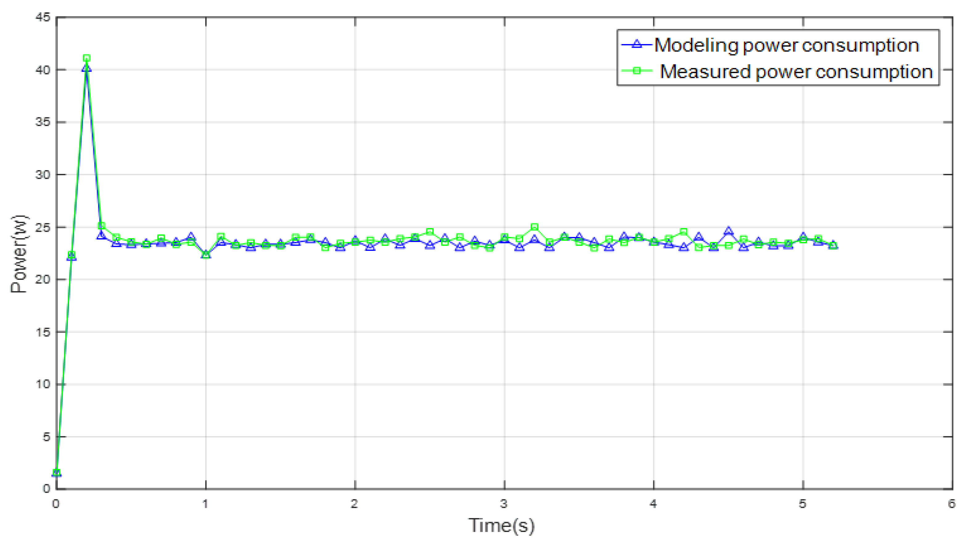
We compared the modeling power consumption of the robot with the actual measured power consumption. The results are shown in the Table 4 and in Figure 13, which show that the accuracy between the modeled and measured values of the robot’s power consumption was above 97%.

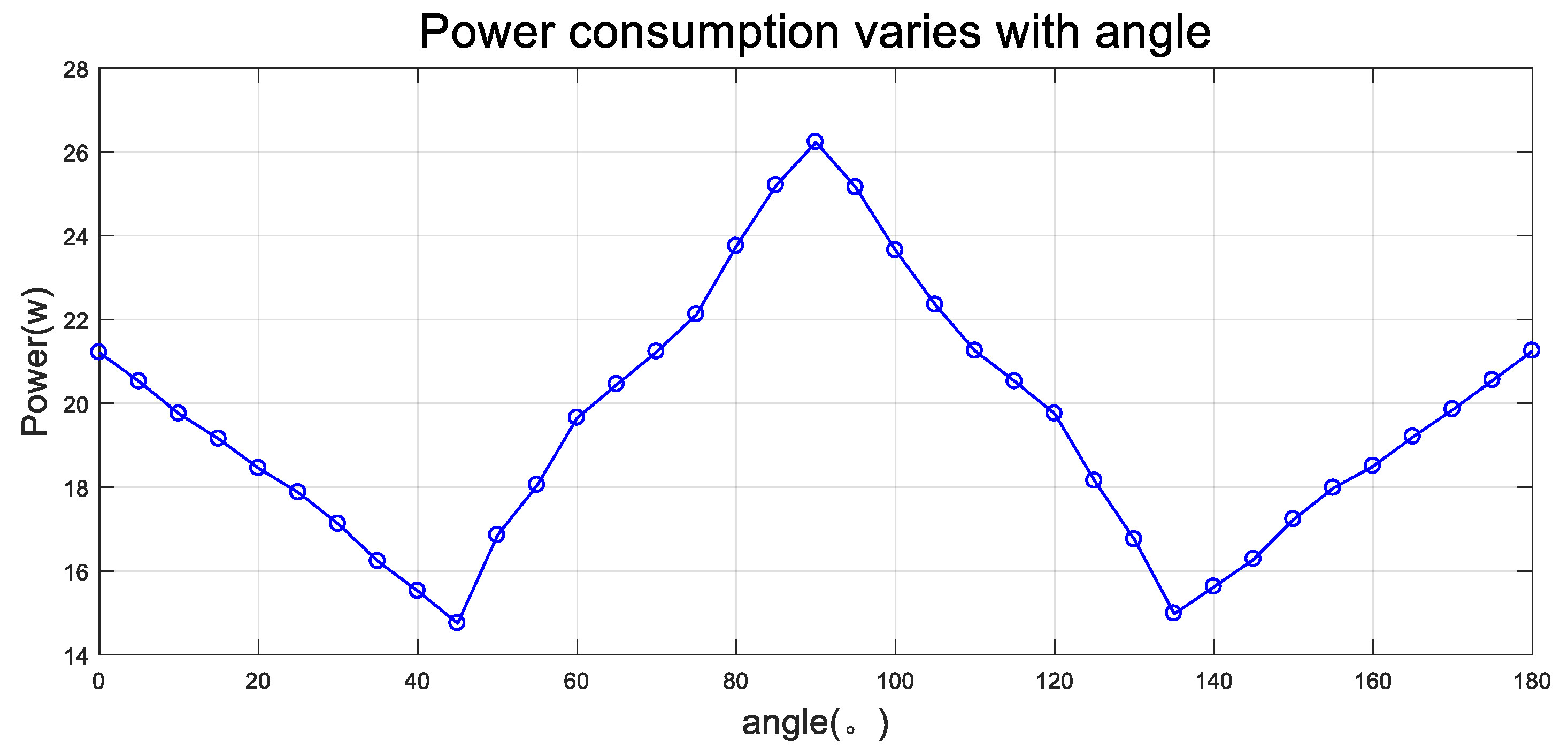
We inferred that the power consumption of the robot was the lowest at a 45° movement angle, and the power consumption of the robot was the highest at a 90° movement angle. In order to verify our judgment, we set the movement angle of the robot to 180°. First, we controlled the precise movement of the robot. In order to ensure our experimental results, we set the difference between each movement angle of the robot to 3°, ensuring the accuracy of our experimental verification.

In order to ensure the accuracy of the robot during the movement, we first analyzed the kinematics and dynamics of the robot before the experiment.

In Figure 14 shows the relationship between the power consumption of the robot and the robot’s translation angle. The robot consumed the least power at 45° and the most power at 90°. In order to verify the robot’s power consumption characteristics, we measured the robot’s power consumption in a 180° range during the measurement process. After measuring, we found that the power consumption of the robot was as we predicted. The robot consumed the least power at 45°, and the robot’s greatest power consumption was symmetric at about 90°.

4. Conclusions and Future Works

According to the symmetry characteristics of the omnidirectional wheels of the FWMR and after theoretical reversal and experimental verification, power consumption characteristics were analyzed in detail during the omnidirectional movement of the FWMR. The results showed that the FWMR consumed the least power when it moved straight ahead and the most power when it moved at an angle of 90° from the front. Because of the structural symmetry of the FWMR, its power consumption in any direction of motion was also symmetrical within a range of 90° to 180°. After verifying this conclusion, the power consumption of the robot was found to be symmetric about 90°.

The establishment of a power consumption model is of great significance to the autonomy of robots. Robots will be able to predict the power consumption of different paths and control methods according to the model. In the course of the robot’s motion, it will be able to choose to move with the minimum power consumption.

In this paper, we summarized the power consumption characteristics of an FWMR in the omnidirectional movement process, but our summary describes only the power consumption of the FWMR in the no-load state and does not account for the center of gravity of the robot in the loaded state. Moreover, the power consumption characteristics of the robot in complex environments (e.g., moving upward and downward) were not analyzed. The focus of the next step will be summarizing and analyzing the power consumption characteristics of robots in complex environments, and deriving a complete set of power models.