Combined Conflict Evidence Based on Two-Tuple IOWA Operators

1
School of Computer Science and Engineering, Northwestern Polytechnical University, Xi’an 710072, China
2
School of Electronics and Information, Northwestern Polytechnical University, Xi’an 710072, China
*
Author to whom correspondence should be addressed.
Symmetry 2019, 11(11), 1369; https://doi.org/10.3390/sym11111369
Submission received: 15 October 2019
/
Revised: 30 October 2019
/
Accepted: 1 November 2019
/
Published: 4 November 2019
Abstract
:Due to poor natural factors and human interference, the information that was obtained by sensors tends to have high uncertainty and high conflict with others. A combination of highly conflicting evidence with Dempster’s rule often produces results that run counter to intuition. To solve the above problem, a conflict evidence combination methodology is proposed in this article, which contains the distance of evidence, classical conflict coefficient, and two-tuple IOWA operator. Both the classical conflict coefficient and Jousselme distance indicate the degree of evidence conflict, and it is clear that the two parameters are symmetrical. First, the two-tuple IOWA operator is proposed. Second, the orness is determined by aggregated data; then, the weighting vector is calculated by a maximal entropy method. Finally, the weighted average is the evidence in the system by a two-tuple IOWA operator; then, the Dempster combination rule is utilized to fuse information. Compared with other existing methods, the presented methodology has high performance when dealing with conflict evidence and has strong anti-interference ability.
1. Introduction
The Dempster–Shafer (D–S) theory of evidence [1,2,3,4,5,6,7] was introduced by Dempster and Shafer [8]. It can efficiently cope with imprecise and uncertain information without transcendental knowledge. Hence, it has been diffusely applied in various scopes, such as information fusion [9,10], decision-making [11,12,13,14,15], pattern recognition [16,17], dependence assessment [18,19], fault diagnosis [20,21,22,23], support vector machine (SVM), and so on. In addition, evidence theory is combined with fuzzy theory to deal with imprecise data and fuzzy information [24,25,26,27], and many studies about problems under fuzzy environment were conducted. In addition, many new approaches based on belief function were proposed [28,29,30]. Thierry et al. [28] proposed the EVCLUS algorithm that constructs a credal partition in such a way that larger dissimilarities between objects correspond to higher degrees of conflict between the associated mass functions. Su et al. [29] extended Dempster’s rule and presented a new rule based on the concept of joint belief distribution to combine dependent bodies of evidence. Xiao [30] proposed an improved conflicting evidence combination approach based on similarity measure and belief function entropy.
In the frame of D–S evidence theory, while dealing with high conflict evidence, the results are contrary to intuition [31,32]. For example, in the real battle field, because of poor natural factors and human interference, the information that was obtained by sensors tends to have high uncertainty and high conflict with others. Due to the high conflict, the application of D–S evidence theory in practice will be limited to a great extent. In recent years, a lot of work on an evidence combination algorithm has emerged to settle the hot issue of high conflict evidence combination [33,34,35,36,37]. The existing processing methods of the conflict information can be categorized into two classifications. One method is to modify Dempster’s rule of combination such as the method of Yager [38], Quan Sun [39], Smets [40], and so on. Another method is to revise the known data information, that is, the classic Dempster’s combination rule should not be modified and the conflict evidence should be preprocessed before the combination. The second category has many representative methods such as Murphy’s method founded on arithmetic mean of bodies of evidence (BOEs) [35] and Deng’s method founded on weighted average BOEs [41].
Thus far, since it is difficult to modify the mathematical framework of evidence theory, the primary work of researchers at home and abroad is to revise the combination rule and BOEs [42,43,44]. These researchers who modify the combination rule argue that the normalization process in the classical Dempster combination rules leads to counterintuitive results [45]. Although modifying a combination rule can settle the problem of counterintuitive results at some level, it usually wrecks the excellent characteristics such as commutativity and associativity. The different combination order will generate different results without commutativity. This leads to the fact that the decision can not be made for the decision maker. In fact, the viewpoint that the counterintuitive results are caused by Dempster’s rule is irrational because outside intervention or sensor failure makes the provided data inaccurate. As argued by Haenni [46], modifying the data information is more rational from the perspective of practicality and philosophy. Based on the analysis above, in order to settle the issue of a combination of high conflict evidence, the idea of modifying the data information is more convenient. That is, the rule itself should not be revised and the evidence to be merged should be revised or pretreated. However, the key issue in this methodology is that the weighting vector is difficult to determine.
From the above analysis, the limitations of the classic Dempster’s combination rule have been investigated. In this article, we proposed a method based on the second idea, a combination methodology of conflict evidence based on evidence distance , classical conflict coefficient k, and a two-tuple IOWA operator is proposed, which adopts the model of modifying the data. In the methodology, the maximum entropy method is utilized to obtain the weighting vector based on the collected evidence.
The organization of this paper is set out as follows: Section 2 briefly introduces the concepts of Dempster–Shafer evidence theory, Jousselme distance, new conflict coefficient, two types of aggregation operators, and a maximum entropy method (MEM). In Section 3, we describe how to obtain the weighting vector and propose the two-tuple-IOWA operator. In Section 4, we present a combination methodology of conflict evidence. In Section 5, two examples are given to illustrate the feasibility of the proposed methodology. Some conclusions are given in Section 6.
2. Preliminaries
2.1. Dempster–Shafer Evidence Theory
Definition 1.
Let Θ be the frame of discernment, with N mutually exclusive alternatives, denoted . A basic probability assignment (BPA) is a mapping m from to [0, 1] that fulfills:
where ϕ represents an empty set and A is a subset of . For subset A: , that is, A is a focal element.
There are two BPAs and in the frame of discernment Θ; then, Dempster’s combination rule is defined as follows:
where
Here, k is a normalization constant, which is considered as a conflict coefficient between two BPAs.
2.2. Jousselme Distance
Definition 2.
Suppose and are two BPAs on the frame of discernment Θ. The Jousselme distance [47], denoted as , is defined below:
Here, D is an square matrix, defined as:
The Jousselme distance can also be represented as:
where ; ; represents vector inner product of and , namely:
where and are the elements of framework Θ (), is the cardinality of common objects between elements and , and is the number of subset of union and .
2.3. New Conflict Coefficient
It is a critical issue to determine the degree of evidence conflict before choosing the suitable approach to fuse the conflict evidence. By now, there is no accurate method to measure the degree of evidence conflict. In recent years, many works on measuring dissimilarity and similarity have emerged. Researchers usually use classical conflict coefficient k or Jousselme distance d to represent the degree of evidence conflict. However, many works have demonstrated that neither d nor k taken alone are adequate to precisely indicate the degree of evidence conflict. Both k and d capture only one aspect of dissimilarity between evidence. When indicating the degree of evidence conflict, it is obvious that the conflict coefficient k and Jousselme distance d are symmetrical. d represents the difference between evidence, and k indicates the non-inclusion between evidence. In addition, only non-inclusive is not enough to accurately determine the degree of evidence conflict; the difference should be taken into account. Taking into account the issues mentioned above, a conflict coefficient is proposed, as follows:
Definition 3.
Definition 3 reveals the relationship between two pieces of evidence: when and , this pair of values shows that there is no conflict between two pieces of evidence. When both k and d have giant values, both of them show that two pieces of evidence are in high conflict. If one of them has low value, there is little contradiction between two pieces of evidence. It can be seen that the smaller the is, the smaller the degree of evidence conflict.
Example 1.
Let be two BPAs on frame such that
In this example, we can see that the two pieces of evidence have three compatible elements and only one incompatible element. Intuitively, it is expected that the similarity between evidence should be larger than the dissimilarity between evidence.
From the results, we can see that indicates that there is no conflict and reveals that the the dissimilarity is larger than the similarity. Therefore, both k and d are irrational.
Then, based on Definition 3, we get
The obtained result reveals that and are partially conflicting, and the dissimilarity is smaller than the similarity, which is consistent with the above analysis.
Example 2.
Let , be two BPAs from two distinct sources on frame and P is a subset of Θ, such that
Take twenty cases as an example, shown in Table 1. The comparison between k and is graphically illustrated in Figure 1. From Figure 1, it can be clearly seen that
(1) The classical conflict coefficient is constant for 20 cases, which reveals that the conflict is small and unchanged. Thus, it is irrational. (2) The new conflict coefficient goes up and down, when the size of A changes. The degree of conflict gets the minimum when , which consists with the intuition.
The two examples demonstrate that the new conflict coefficient can efficiently characterize the conflict between pieces of evidence. In addition, it overcomes the drawback of classical conflict coefficient k and evidence distance d to some extent.
2.4. OWA Operator and IOWA Operator
Definition 4.
By extending the OWA operator, Yager and Filev introduced the definition of the induced OWA(IOWA) as follows:
where is the order inducing variable and is the argument variable.
To estimate the extent of aggregation such as or operation, which can be regarded as support in the decision-making process. Yager [51] introduced value of , which is defined as
Yager [48] introduced entropy of , which is defined as follows:
where represents entropy of . The more uniform the distribution of each weight in the weight vector, the greater the entropy.
2.5. Maximum Entropy Method
O’Hagan [52] introduced the maximum entropy method (MEM). This approach needs the settlement of the following constrained nonlinear optimization model:
The OWA operator weighting vectors can be obtained by the MEM for a given level of orness. It is easy to find three special OWA weighting vectors for three special levels of orness.
If , then the associated weighting vecor is
If , then the associated weighting vecor is
If , then the associated weighting vecor is
3. Two-Tuple IOWA Operator and the Determine Weighting Vector of Multi-Source BOEs
The following sections will present the proposed approach from two aspects. In the first part of the proposed operator, a two-tuple IOWA operator as the order inducing variables is proposed. In the second component, the weighting vector is determined by a maximum entropy method. This is a key step that leads to a valid combination with evidence theory.
3.1. Two-Tuple IOWA Operator
According to Equation (10), the IOWA operator is . Suppose that there are two OWA pairs and , where (i, j = 1, 2,..., N). Thus, it can not order the arguments and only based on inducing variable and . Assume there is another order inducing variable vector and , hence we can order the arguments and based on variable and . Therefore, we refer to the two-tuples variable value as the order inducing variables. The definition of modified IOWA operator is as follows:
Definition 5.
If , then ; if and , then . In other words, first we order the arguments based on the value. If , we order the arguments based on and .
The following example illustrates the approach.
Example 3.
Suppose there are five two-tuple OWA pairs , and the weights of each pair are :
The first step is to sort the two-tuple OWA pairs according to two-tuple ordering inducing variable . The ordered result is obtained as follows:
According to Equation (14), we obtain:
Suppose that we have two two-tuple OWA pairs and . However, and , thus we cannot order the two two-tuple OWA pairs according to two-tuple order inducing variables.
Example 4.
Consider aggregation of the object
with the weighting vector .
Performing the ordering of the objects, we obtain
As for this case, we can not order , based on Definition 5. We argue they have identical importance, namely, they should have the same weight. Thus, we can replace the corresponding two weights by their average . The associated weighting vector is replaced by the modified weighting vector .
According to Equation (14), we obtain:
In particular, assume that two two-tuple OWA pairs and are exactly the same, namely, , and . For example, the second two-tuple OWA pairs in Example 4 changes into ; the other two-tuple OWA pairs and weighting vector are not modified.
As for this case, we can not order , as well. We can deal with them by the same process in Example 4. Since they are totally the same, this course can be virtually expressed to assign the sum of corresponding two weights to one two-tuple OWA pair and assign zero to the other one. That is,
In other words, the weight is replaced by modified weight .
Similarly, if more than two two-tuple OWA pairs are totally the same, we assign the sum of corresponding weights to one of two-tuple OWA pairs and assign zero to others.
3.2. The Determination of Associated Weight of BOEs
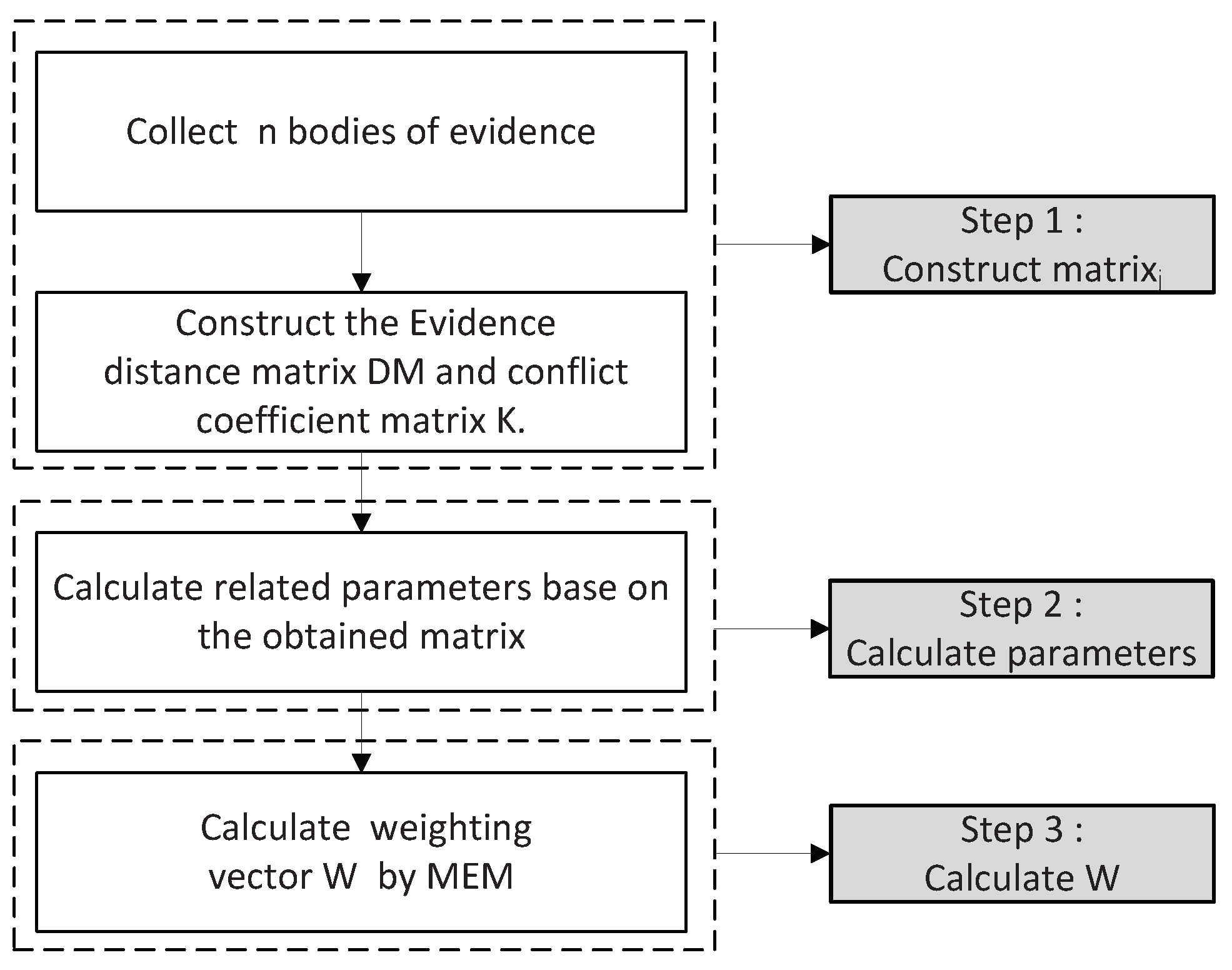
The flowchart of the determination of associated weight of BOEs is presented as Figure 2. The proposed method for determining weight by the maximum entropy method is now presented as follows:
assume that there are n bodies of evidence. The evidence set is . The conflict coefficient and evidence distance can be obtained by Equations (2) and (5). Then, the conflict coefficient matrix and evidence distance matrix could be constructed as follows:
where is the classical conflict coefficient between evidence and evidence :
where is the Jousselme distance between evidence and evidence .
Definition 6.
The average conflict coefficient and the average evidence distance of evidence are defined respectively as follows:
Definition 7.
For all the evidence, calculate their corresponding and , respectively, and then normalize them, shown as follows:
where is called global normalization conflict coefficient, is called global normalization evidence distance. Since the definition of new conflict coefficient is , the conflict coefficient matrix can be calculated by matrix K and , as follows:
Definition 8.
The new global normalization conflict coefficient of evidence is defined as follows:
In recent years, the OWA operator and IOWA operator have received increasing attention [53] and have been used in a wide range of applications including group decision-making [54,55], neural networks [56,57,58,59], database mining [60], etc.
However, there are some drawbacks when researchers aggregate data by OWA operator or IOWA operator. In general, the weighting vector in OWA and IOWA is irrelevant to its corresponding input, so the weight vector can be considered to be a relatively independent part. For example, researchers usually determine OWA operator weighting vector W by MEM, but the value of constraint condition is given by researchers. Thus, there is human preference in the value. Since both the argument variables and the interrelationships between them are not considered in the producing course of weighting vector, the obtained weighting vector has a strong subjective randomness. Therefore, the determined weighting vector is unreasonable. For instance, although there are two distinct sets of data, the obtained weighting vectors must be the same if a researcher gives the same value. Hence, it is not rational since the obtained weighting vector cannot reflect the objectivity of given data. In order to reduce the intervention of human factor when determining weighting vector, and to reflect the the objectivity of the obtained weighting vector, we shall determine the value based on the argument variables and their interrelationships. According to such an idea, this paper determines the value based on the objective data from the BOEs to avoid the subjective randomness.
This paper constructs the relationship between global normalization new conflict coefficient and constraint of MEM. That is to say, is determined by . Clearly, the larger the of BOEs, the greater the total degree of conflict between evidence. We argue that the higher the total degree of conflict is, the smaller the credibility difference between BOEs is. If the is larger, the weight of BOE should be closer. Namely, the weighting vector is closer to . At the same time, the corresponding is closer to 0.5. Furthermore, we should assign weight to each BOE according to the average conflict coefficient and average evidence distance of BOE . The smaller the and of BOE , the larger the corresponding credibility. That is, BOE can greatly affect the final result. Therefore, the endowed weight should be larger. indicates that the BOEs in system are totally contradictory. In this case, we argue that every BOE has the same credibility, namely , . Otherwise, the smaller the is, the smaller the total degree of conflict of BOEs. That is to say, the difference between evidence is smaller. All of the evidence can be represented by one or more pieces of evidence. Partial evidence, whose and values are smaller, takes most of the weight, namely the corresponding is close to 1 and W is close to . If , then the n BOEs are totally identical. Thus, any one of the BOEs can be used to represent all the evidence. Without loss of generality, we endow all weight to the first piece of evidence, namely , . In summary, the smaller the , the larger the . If , then , ; if , then , .
According to the analysis above, the relationship between and is constructed as follows:
where
The parameter is determined, then the weighting vector can be obtained by the maximum entropy method.
4. New Combination Approach of Conflict Evidence
This paper is ready to aggregate the evidence in the system by a two-tuple IOWA operator proposed in Section 3. The proposed method can be enumerated at every step as follows:
step1: Calculate the Jousselme distance , the classic conflict coefficient , and construct the evidence distance matrix and conflict coefficient matrix K.
step2: According to Definitions 6–8, calculate , , and based on the obtained matrix and K.
step3: According to Equation (30), calculate base on the obtained in step 2. Then, the weighting vector can be obtained by MEM.
step4: First, construct two-tuple order inducing variable by and . Then, construct a two-tuple OWA pair , where is the argument variable (BPA of evidence ).
step5: According to Equation (14), the weighted average evidence in the system is given as:
step6: When n pieces of evidence are combined using the classic Dempster rule, there are combined times. Then, the final combination result can be obtained.
5. Example and Analysis
In this section, the proposed combination method is applied in two examples to illustrate the effectiveness of method.
Example 5.
Suppose that a target was detected in combat air domain. The target was identified as an enemy by military Identification Friend or Foe. Five different sensors such as airborne early warning radar (AEW radar) and electronic warfare support measure (EMS) provide the type information of the target, where the frame of discernment is . Sometimes, five sets of evidence are collected from five different sensors. Their BPAs are given as follows:
Supposing that the second sensor was interrupted by the electromagnetic interference of enemy, the BPA provided by the second sensor changes into
It is clear that the BPA provided by the second sensor highly conflicts with others. This BPA is called “bad” evidence. Applying different combination rules, we obtain the different combination results as shown in Table 2.
From Table 2, it can be clearly seen that, when combining the conflict evidence with traditional Dempster’s combination rules, the obtained results are contrary to intuition. The results of the Dempster’s combination rules are different from those produced by other methods. Yager’s combination results cannot recognize the target when there are two BOEs . With incremental evidence, Yager’s method, Murphy’method, Deng’s method, and the proposed method can produce legitimate results. However, the uncertainty of other three methods are larger than the proposed method, which is better for the decision-maker to make decisions. Moreover, although the uncertainty of Yager’s approach decreases with the amount of evidence increasing, the underspeed is much lower than the latter three methods. When the system collects five pieces of evidence , the of Yager is 0.774, this is much smaller than the latter three methods. To compare with Murphy’s method and Deng’s method, the proposed method converges faster. In the proposed method, the difference between and other BPAs is greater. Obviously, the proposed method is very obvious to determine the most likely target. Murphy’s simple average does not take into account the degree of correlation between evidence collected from multi-sources. The weight assigned to each evidence is equivalent, thus the “bad” evidence will negatively affect the final combination results. However, Deng’s weighted average method considers the difference between evidence, which reduces the weight of “bad” evidence; therefore, it greatly reduces the impact of “bad” evidence on the final combined outcome. It greatly offsets the shortage of Murphy’s method. Compared with Deng’s method, the weight generating method of the proposed method was further improved, hence the results of the proposed method are better than Deng’s. By using the proposed approach, the obtained results are close to people’s expectation.
Example 6.
Suppose that the fifth sensor also interferes since the enemy strengthened the electromagnetic interference. The BPA provided by the fifth sensor changes into:
The different combination results with two “bad” pieces of evidence are shown in Table 3; it can be seen that the combination results of both Dempster and Yager are illogical. Compared with the proposed method, although the recognized target of both Murphy and Deng are A, their uncertainty has increased a lot. In other words, the stability (anti-interference ability) of the proposed method is greater than other approaches.
In conclusion, the proposed combination method can efficiently cope with the combination problem of high conflict evidence. In addition, the proposed method converges faster than other methods and the anti-interference ability of the proposed method is stronger, which can reduce the uncertainty of the final recognized target.
6. Conclusions
When the evidence is highly conflicting, the classical Dempster combination rules are used to obtain the results that are contrary to intuition. After analysis of different combination approaches, a combination method based on distance of evidence d, classical conflict coefficient k, and two-tuple IOWA operator was proposed in this paper. In this paper, the distance of evidence and conflict coefficient are used to determine the conflict coefficient, which can reflect the degree of conflict between the evidence more comprehensively. The method of obtaining the weighting vector by maximum entropy is further improved, hence the proposed method can obtain more intuitive results. The proposed method retains many great characteristics of Dempster’s method, such as commutativity and associativity. In addition, compared with existing methods, the anti-interference ability of the proposed method is stronger, which can enhance the reliability and rationality of the final results when dealing with conflicting evidence.
Author Contributions
Y.Z. wrote this paper, X.Q. and X.Z. reviewed and improved this article, Y.Z., X.Q., and X.Z. discussed and analyzed the numerical results.
Funding
The work is partially supported by the National Natural Science Foundation of China (Program No. 61671384).
Conflicts of Interest
The authors declare no conflict of interest.
References
- Dempster, A.P. Upper and lower probabilities induced by a multivalued mapping. Ann. Math. Stat. 1967, 38, 325–339. [Google Scholar] [CrossRef]
- Ye, F.; Chen, J.; Li, Y. Improvement of DS evidence theory for multi-sensor conflicting information. Symmetry 2017, 9, 69. [Google Scholar]
- Shafer, G. A Mathematical Theory of Evidence; Princeton University Press: Princeton, NJ, USA, 1976; Volume 42. [Google Scholar]
- He, Z.; Jiang, W. A new belief Markov chain model and its application in inventory prediction. Int. J. Prod. Res. 2018, 56, 2800–2817. [Google Scholar] [CrossRef]
- Denoeux, T. 40 years of Dempster-Shafer theory. Int. J. Approx. Reason. 2016, 79, 1–6. [Google Scholar] [CrossRef]
- Chen, J.; Ye, F.; Jiang, T.; Tian, Y. Conflicting information fusion based on an improved ds combination method. Symmetry 2017, 9, 278. [Google Scholar] [CrossRef]
- Jiang, W. A correlation coefficient for belief functions. Int. J. Approx. Reason. 2018, 103, 94–106. [Google Scholar] [CrossRef] [Green Version]
- Fu, C.; Xu, D.L.; Xue, M. Determining attribute weights for multiple attribute decision analysis with discriminating power in belief distributions. Knowl.-Based Syst. 2018, 143, 127–141. [Google Scholar] [CrossRef] [Green Version]
- Xiao, F. Multi-sensor data fusion based on the belief divergence measure of evidences and the belief entropy. Inf. Fusion 2019, 46, 23–32. [Google Scholar] [CrossRef]
- Su, X.; Li, L.; Shi, F.; Qian, H. Research on the Fusion of Dependent Evidence Based on Mutual Information. IEEE Access 2018, 6, 71839–71845. [Google Scholar] [CrossRef]
- Deng, X.; Jiang, W. D number theory based game-theoretic framework in adversarial decision making under a fuzzy environment. Int. J. Approx. Reason. 2019, 106, 194–213. [Google Scholar] [CrossRef]
- Fei, L.; Deng, Y.; Hu, Y. DS-VIKOR: A New Multi-criteria Decision-Making Method for Supplier Selection. Int. J. Fuzzy Syst. 2018. [Google Scholar] [CrossRef]
- He, Z.; Jiang, W. An evidential dynamical model to predict the interference effect of categorization on decision making. Knowl.-Based Syst. 2018, 150, 139–149. [Google Scholar] [CrossRef]
- Xiao, F. A multiple criteria decision-making method based on D numbers and belief entropy. Int. J. Fuzzy Syst. 2019, 21, 1144–1153. [Google Scholar] [CrossRef]
- Fu, C.; Chang, W.; Xue, M.; Yang, S. Multiple criteria group decision making with belief distributions and distributed preference relations. Eur. J. Oper. Res. 2019, 273, 623–633. [Google Scholar] [CrossRef]
- Han, Y.; Deng, Y. An Evidential Fractal AHP target recognition method. Def. Sci. J. 2018, 68, 367–373. [Google Scholar] [CrossRef]
- Cui, H.; Liu, Q.; Zhang, J.; Kang, B. An improved deng entropy and its application in pattern recognition. IEEE Access 2019, 7, 18284–18292. [Google Scholar] [CrossRef]
- Zhang, X.; Mahadevan, S. A game theoretic approach to network reliability assessment. IEEE Trans. Reliab. 2017, 66, 875–892. [Google Scholar] [CrossRef]
- Kang, B.; Zhang, P.; Gao, Z.; Chhipi-Shrestha, G.; Hewage, K.; Sadiq, R. Environmental assessment under uncertainty using Dempster–Shafer theory and Z-numbers. J. Ambient. Intell. Humaniz. Comput. 2019. [Google Scholar] [CrossRef]
- Jiang, W.; Xie, C.; Zhuang, M.; Tang, Y. Failure Mode and Effects Analysis based on a novel fuzzy evidential method. Appl. Soft Comput. 2017, 57, 672–683. [Google Scholar] [CrossRef]
- Zhang, H.; Deng, Y. Engine fault diagnosis based on sensor data fusion considering information quality and evidence theory. Adv. Mech. Eng. 2018, 10. [Google Scholar] [CrossRef] [Green Version]
- Xiao, F. A Hybrid Fuzzy Soft Sets Decision Making Method in Medical Diagnosis. IEEE Access 2018, 6, 25300–25312. [Google Scholar] [CrossRef]
- Zhang, y.; Jiang, W.; Deng, X. Fault diagnosis method based on time domain weighted data aggregation and information fusion. Int. J. Distrib. Sens. Netw. 2019, 15. [Google Scholar] [CrossRef]
- Song, Y.; Wang, X. A new similarity measure between intuitionistic fuzzy sets and the positive definiteness of the similarity matrix. Pattern Anal. Appl. 2017, 20, 215–226. [Google Scholar] [CrossRef]
- Deng, X.; Jiang, W.; Wang, Z. Zero-sum polymatrix games with link uncertainty: A Dempster-Shafer theory solution. Appl. Math. Comput. 2019, 340, 101–112. [Google Scholar] [CrossRef]
- Dubois, D.; Liu, W.; Ma, J.; Prade, H. The basic principles of uncertain information fusion. An organised review of merging rules in different representation frameworks. Inf. Fusion 2016, 32, 12–39. [Google Scholar] [CrossRef]
- Han, D.; Yang, Y.; Han, C. Evidence updating based on novel Jeffrey-like conditioning rules. Int. J. Gen. Syst. 2017, 46, 587–615. [Google Scholar] [CrossRef]
- Denœux, T.; Sriboonchitta, S.; Kanjanatarakul, O. Evidential clustering of large dissimilarity data. Knowl.-Based Syst. 2016, 106, 179–195. [Google Scholar] [CrossRef] [Green Version]
- Su, X.; Li, L.; Qian, H.; Mahadevan, S.; Deng, Y. A new rule to combine dependent bodies of evidence. Soft Comput. 2019, 23, 9793–9799. [Google Scholar] [CrossRef]
- Xiao, F. An Improved Method for Combining Conflicting Evidences Based on the Similarity Measure and Belief Function Entropy. Int. J. Fuzzy Syst. 2018, 20, 1256–1266. [Google Scholar] [CrossRef]
- Zhang, W.; Deng, Y. Combining conflicting evidence using the DEMATEL method. Soft Comput. 2018. [Google Scholar] [CrossRef]
- Jiang, W.; Huang, C.; Deng, X. A new probability transformation method based on a correlation coefficient of belief functions. Int. J. Intell. Syst. 2019, 34, 1337–1347. [Google Scholar] [CrossRef]
- Deng, X.; Jiang, W. A total uncertainty measure for D numbers based on belief intervals. Int. J. Intell. Syst. 2019. [Google Scholar] [CrossRef]
- Lefevre, E.; Colot, O.; Vannoorenberghe, P. Belief function combination and conflict management. Inf. Fusion 2002, 3, 149–162. [Google Scholar] [CrossRef]
- Murphy, C.K. Combining belief functions when evidence conflicts. Decis. Support Syst. 2000, 29, 1–9. [Google Scholar] [CrossRef]
- Smets, P. Analyzing the combination of conflicting belief functions. Inf. Fusion 2007, 8, 387–412. [Google Scholar] [CrossRef]
- Deng, X.; Han, D.; Dezert, J.; Deng, Y.; Shyr, Y. Evidence combination from an evolutionary game theory perspective. IEEE Trans. Cybern. 2016, 46, 2070–2082. [Google Scholar] [CrossRef] [PubMed]
- Yager, R.R. On the Dempster-Shafer framework and new combination rules. Inf. Sci. 1987, 41, 93–137. [Google Scholar] [CrossRef]
- Sun, Q.; Ye, X.q.; Gu, W.k. A new combination rules of evidence theory. Acta Electron. Sin. 2000, 28, 117–119. [Google Scholar]
- Smets, P. Data fusion in the transferable belief model. In Proceedings of the Third International Conference on Information Fusion (FUSIon 2000), Paris, France, 10–13 July 2000; Volume 1, pp. PS21–PS33. [Google Scholar]
- Yong, D.; WenKang, S.; ZhenFu, Z.; Qi, L. Combining belief functions based on distance of evidence. Decis. Support Syst. 2004, 38, 489–493. [Google Scholar] [CrossRef]
- Deng, X.; Jiang, W. Evaluating green supply chain management practices under fuzzy environment: A novel method based on D number theory. Int. J. Fuzzy Syst. 2019, 21, 1389–1402. [Google Scholar] [CrossRef]
- Xiao, F. A novel multi-criteria decision making method for assessing health-care waste treatment technologies based on D numbers. Eng. Appl. Artif. Intell. 2018, 71, 216–225. [Google Scholar] [CrossRef]
- Huang, Z.; Yang, L.; Jiang, W. Uncertainty measurement with belief entropy on the interference effect in the quantum-like Bayesian Networks. Appl. Math. Comput. 2019, 347, 417–428. [Google Scholar] [CrossRef]
- He, Z.; Jiang, W. An evidential Markov decision making model. Inf. Sci. 2018, 467, 357–372. [Google Scholar] [CrossRef] [Green Version]
- Haenni, R. Are alternatives to Dempster’s rule of combination real alternatives?: Comments on “About the belief function combination and the conflict management problem”—-Lefevre et al. Inf. Fusion 2002, 3, 237–239. [Google Scholar] [CrossRef]
- Jousselme, A.L.; Grenier, D.; Bossé, É. A new distance between two bodies of evidence. Inf. Fusion 2001, 2, 91–101. [Google Scholar] [CrossRef]
- Yager, R.R. On ordered weighted averaging aggregation operators in multicriteria decisionmaking. In Readings in Fuzzy Sets for Intelligent Systems; Elsevier: Amsterdam, The Netherlands, 1993; pp. 80–87. [Google Scholar]
- Fei, L.; Wang, H.; Chen, L.; Deng, Y. A new vector valued similarity measure for intuitionistic fuzzy sets based on OWA operators. Iran. J. Fuzzy Syst. 2019, 16, 113–126. [Google Scholar]
- Pan, L.; Deng, Y. A New Belief Entropy to Measure Uncertainty of Basic Probability Assignments Based on Belief Function and Plausibility Function. Entropy 2018, 20, 842. [Google Scholar] [CrossRef]
- Yager, R.R.; Kacprzyk, J. The Ordered Weighted Averaging Operators: Theory and Applications; Springer Science & Business Media: Berlin/Heidelberg, Germany, 2012. [Google Scholar]
- O’Hagan, M. Aggregating template or rule antecedents in real-time expert systems with fuzzy set logic. In Proceedings of the Twenty-Second Asilomar Conference on Signals, Systems and Computers, Pacific Grove, CA, USA, 31 October–2 November 1988; Volume 2, pp. 681–689. [Google Scholar]
- Chiclana, F.; Herrera-Viedma, E.; Herrera, F.; Alonso, S. Some induced ordered weighted averaging operators and their use for solving group decision-making problems based on fuzzy preference relations. Eur. J. Oper. Res. 2007, 182, 383–399. [Google Scholar] [CrossRef]
- Zeng, S.; Merigo, J.M.; Su, W. The uncertain probabilistic OWA distance operator and its application in group decision making. Appl. Math. Model. 2013, 37, 6266–6275. [Google Scholar] [CrossRef]
- Merigo, J.M.; Engemann, K.J.; Palacios-Marques, D. Decision making with Dempster-Shafer belief structure and the OWAWA operator. Technol. Econ. Dev. Econ. 2013, 19, S100–S118. [Google Scholar] [CrossRef]
- Cho, S.B. Fuzzy aggregation of modular neural networks with ordered weighted averaging operators. Int. J. Approx. Reason. 1995, 13, 359–375. [Google Scholar] [Green Version]
- Jiang, W.; Cao, Y.; Deng, X. A Novel Z-network Model Based on Bayesian Network and Z-number. IEEE Trans. Fuzzy Syst. 2019. [Google Scholar] [CrossRef]
- Geng, J.; Ma, X.; Zhou, X.; Wang, H. Saliency-Guided Deep Neural Networks for SAR Image Change Detection. IEEE Trans. Geosci. Remote. Sens. 2019, 1–13. [Google Scholar] [CrossRef]
- Zhang, X.; Mahadevan, S.; Sankararaman, S.; Goebel, K. Resilience-based network design under uncertainty. Reliab. Eng. Syst. Saf. 2018, 169, 364–379. [Google Scholar] [CrossRef]
- Peng, Y.; Zhang, Y.; Tang, Y.; Li, S. An incident information management framework based on data integration, data mining, and multi-criteria decision making. Decis. Support Syst. 2011, 51, 316–327. [Google Scholar] [CrossRef]
Figure 1.
Comparison of d and .
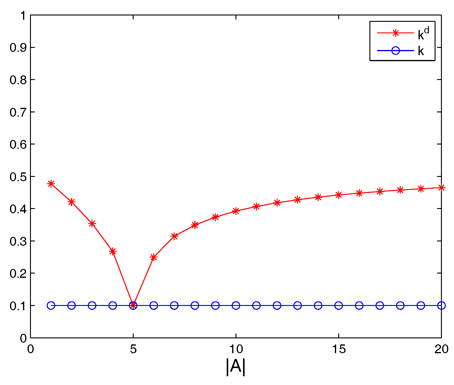
Figure 2.
The flowchart of the proposed method.

Table 1.
Comparison of , k and of and when subset A changes.
| Case | k | ||
|---|---|---|---|
| 0.8544 | 0.1000 | 0.4772 | |
| 0.7416 | 0.1000 | 0.4208 | |
| 0.6083 | 0.1000 | 0.3541 | |
| 0.4359 | 0.1000 | 0.2680 | |
| 0.1000 | 0.1000 | 0.1000 | |
| 0.4000 | 0.1000 | 0.2500 | |
| 0.5292 | 0.1000 | 0.3146 | |
| 0.5990 | 0.1000 | 0.3495 | |
| 0.6481 | 0.1000 | 0.3740 | |
| 0.6848 | 0.1000 | 0.3924 | |
| 0.7135 | 0.1000 | 0.4068 | |
| 0.7365 | 0.1000 | 0.4183 | |
| 0.7555 | 0.1000 | 0.4277 | |
| 0.7714 | 0.1000 | 0.4357 | |
| 0.7849 | 0.1000 | 0.4425 | |
| 0.7965 | 0.1000 | 0.4482 | |
| 0.8066 | 0.1000 | 0.4533 | |
| 0.8155 | 0.1000 | 0.4577 | |
| 0.8233 | 0.1000 | 0.4617 | |
| 0.8304 | 0.1000 | 0.4652 |
Table 2.
Results of different combination rules of evidence with one bad piece of evidence.
| BOEs | Approach | Target | |||||
|---|---|---|---|---|---|---|---|
| Dempster | 0 | 0.8571 | 0.1429 | 0 | 0 | B | |
| Yager [38] | 0 | 0.1800 | 0.0300 | 0 | 0.7900 | Θ | |
| Murphy [35] | 0.1543 | 0.7469 | 0.0988 | 0 | 0 | B | |
| Deng [41] | 0.1543 | 0.7469 | 0.0988 | 0 | 0 | B | |
| Proposed | 0.1543 | 0.7469 | 0.0988 | 0 | 0 | B | |
| Dempster | 0 | 0.6316 | 0.3684 | 0 | 0 | B | |
| Yager [38] | 0.4345 | 0.097 | 0.0105 | 0.2765 | 0.1815 | A | |
| Murphy [35] | 0.5568 | 0.3562 | 0.0782 | 0.0088 | 0 | A | |
| Deng [41] | 0.6500 | 0.2547 | 0.0858 | 0.0095 | 0 | A | |
| Proposed | 0.7429 | 0.1489 | 0.1019 | 0.0067 | 0 | A | |
| Dempster | 0 | 0.3288 | 0.6712 | 0 | 0 | C | |
| Yager [38] | 0.6430 | 0.0279 | 0.0037 | 0.1603 | 0.1652 | A | |
| Murphy [35] | 0.8653 | 0.0891 | 0.0382 | 0.0074 | 0 | A | |
| Deng [41] | 0.9305 | 0.0274 | 0.0339 | 0.0082 | 0 | A | |
| Proposed | 0.9638 | 0.0049 | 0.0184 | 0.0139 | 0 | A | |
| Dempster | 0 | 0.1404 | 0.8596 | 0 | 0 | C | |
| Yager [38] | 0.7740 | 0.0193 | 0.0011 | 0.0977 | 0.1080 | A | |
| Murphy [35] | 0.9688 | 0.0156 | 0.0127 | 0.0029 | 0 | A | |
| Deng [41] | 0.9846 | 0.0024 | 0.0098 | 0.0032 | 0 | A | |
| Proposed | 0.9897 | 0.0002 | 0.0043 | 0.0058 | 0 | A |
© 2019 by the authors. Licensee MDPI, Basel, Switzerland. This article is an open access article distributed under the terms and conditions of the Creative Commons Attribution (CC BY) license (http://creativecommons.org/licenses/by/4.0/).
Share and Cite
MDPI and ACS Style
Zhou, Y.; Qin, X.; Zhao, X. Combined Conflict Evidence Based on Two-Tuple IOWA Operators. Symmetry 2019, 11, 1369. https://doi.org/10.3390/sym11111369
AMA Style
Zhou Y, Qin X, Zhao X. Combined Conflict Evidence Based on Two-Tuple IOWA Operators. Symmetry. 2019; 11(11):1369. https://doi.org/10.3390/sym11111369
Chicago/Turabian StyleZhou, Ying, Xiyun Qin, and Xiaozhe Zhao. 2019. "Combined Conflict Evidence Based on Two-Tuple IOWA Operators" Symmetry 11, no. 11: 1369. https://doi.org/10.3390/sym11111369
Note that from the first issue of 2016, this journal uses article numbers instead of page numbers. See further details here.