Vector-Coupled Flight Controller Design Based on Multivariable Backstepping Sliding Mode

Abstract

This study aims to address the issues of the simultaneous control of the angle of attack, sideslip angle, and airspeed of a flight in a vectorial form. A vector controller, with a symmetry structure, is developed to transform the attitude and speed control problem into a space-vector tracking problem. We first establish flight vector-coupled dynamics, i.e., describe velocity and angular-velocity vectors in a body-fixed frame, and then propose a multivariable backstepping sliding mode control algorithm along with nonlinear disturbance observers for the vectorial dynamics. The theoretical analysis ensures that the states of the system can be enforced to reach a small neighborhood of the desired sliding manifold. The results of the numerical simulation illustrate the effectiveness and robustness of the combined vector-control scheme.

1. Introduction

There are many interesting and challenging problems with respect to the control of modern aircraft. These include, but are not limited to, the cross-coupling of dynamics [1], non-minimum phase behavior [2], constraints on the control inputs as a result of position and rate limits [3], and high nonlinearity and uncertainty [4] in flight equations. Moreover, the performance of a flight control system is expected to be very high, and the demands for flight safety have dictated the development of the robust control designs [5].

Traditionally, flight control systems were developed based on the “small perturbation theory”. This theory follows the assumption that flight dynamics are time-invariant and linear around the operating points, while the longitudinal dynamics are independent of the lateral ones. Then, the equations of motion can be decoupled and addressed separately with linear control methods such as proportion integration differentiation (PID) control [6] and linear quadratic control [7,8]. However, the performance of flight control systems deteriorates owing to the un-modeled terms of the nonlinearities intrinsic to flight dynamics, and the cross-coupling between the longitudinal and lateral motions, which become crucial under an ultra condition, such as a large angle of attack (AOA) or speedy rolling [9].

To overcome the disadvantages of the linear methods, nonlinear control laws have been developed rapidly in the past decades. Feedback linearization is one of the most widely used amongst such methods [10,11]. However, the primary drawback of these methods is that all nonlinearities of a control system must be known for feedback linearization [12]. However, the effective and robust nonlinear control methods that do not require all nonlinearities to be accurate have been used in flight control. Sliding mode control [13,14,15], disturbance observer-enhanced control [16,17], model predictive control [18], adaptive backstepping [19], and dynamic surface control [20] are some nonlinearities that have been considered.

The design of controls of flights have achieved various degrees of success. However, there are several challenges that deserve further research:

• Cross-coupling that is inherent to flight dynamics. In previous studies [13,14,16,17,18,19,20,21], the models used to design flight control were decoupled into a scalar form, i.e., state equations with velocity, AOA, sideslip angle, roll rate, pitch rate, and yaw rate, and multiple single-channel controllers were designed. During the decoupling process, some coupling components terms are first calculated/estimated and then compensated for, while the other coupling terms may be disregarded owing to their negligible influence. However, this is a conservative method because the coupling terms may include the control input.
• Design of control laws that ensure the stability of the whole control system. In some studies [22,23], the design of the control systems is based on the assumption with “timescale separation”, wherein the slow attitude dynamics are separated from the fast angular-rate dynamics. The outer and inner controllers correspond to the slow and fast subsystems, respectively. They can be designed individually to simplify the complexity of the control system. However, the inherent weakness of this framework is that the overall system’s stability cannot be achieved theoretically.
• Uncertainties regarding various disturbances, including external disturbances, un-modeled dynamics, and parameter uncertainties. Balancing the robustness and the control performance of an aircraft control system during the design process is important. The robustness and control performance of a control system have an inverse relationship, i.e., a more robust controller implies more certain attenuation; however, the robustness is obtained by sacrificing the nominal control performance to a certain extent.

Motivated by the aforementioned challenge, and for a multivariable backstepping sliding mode approach through disturbance estimation for the flight control systems within multivariable design, this study aimed to make the following contributions:

• We model the flight dynamics using a body-fixed frame in the vectorial form and consider both matched and unmatched disturbances. The attitude control of an aircraft, along with the total velocity, can be converted into a space-vector tracking equation. The triplet airspeed ($V_T$), AOA ($\alpha$) and sideslip angle ($\beta$) are controlled simultaneously in a vectorial manner. This also allows us to deal with the cross-term actively and correctly. A key aspect of this study is the active use of the cross-coupling in terms of flight dynamics instead of decoupling and passive suppression and compensation.
• The control-oriented model has a lower-triangular form. Then, the structure of a Lyapunov-based backstepping approach [24,25] is used in this study to ensure the stability of the closed-loop system theoretically. This work establishes a combined multivariable backstepping sliding mode controller, along with nonlinear disturbance observers. The disturbance observers enhance the scheme of construction of the control law by combining the backstepping sliding mode control feedback with disturbance estimation, based on straightforward and feedforward compensation. Unlike similar works [12,16,17,18,19], the developed controller not only avoids solving complex matrix equations and treating inverse matrixes, but also fully realizes vector-coupled control.
• The developed control structure is concise and aesthetically appealing compared with traditional control structures that use a decoupled collection of single variables. The combined control scheme has a symmetry structure and each term is meaningful, and this feature is significant in that the control parameters can be adjusted in each term directively.

The remainder of this paper is organized as follows. The control-oriented model of the flight dynamics, established in a vectorial manner, is given in Section 2. The multivariable backstepping sliding mode controller, along with the nonlinear disturbance observers, is proposed based on the vectorial scheme in Section 3. The performance of the developed control algorithm is illustrated through simulations in Section 4, and conclusions are drawn in Section 5.

2. Modelling

To describe the flight motion in this study, three coordinates need to be defined as follows:

• Body-fixed Frame: ${\Sigma }_b$, the reference frame with the origin at the gravity center and axes pointing forward, over the right wing, and down (relative to the pilot).
• Inertial Frame: ${\Sigma }_i$, the reference frame with a specific ground origin and axes pointing the North, East, and down to the Earth center.
• Wind Frame: ${\Sigma }_w$, the reference frame with the origin at the gravity center and the x-axis pointing to the velocity direction of the flight. The orientation of this frame relative to the body-fixed frame is determined by AOA ($\alpha$) and sideslip angle ($\beta$). The lift, drag, and side forces are defined naturally in this reference frame, respectively.

Figure 1 depicts an aircraft model [26] with the defined frames.The controlled aircraft is assumed to be a rigid body with mass m, and the motion in a body-fixed coordinate system with the origin at the center of mass, which can be described as:

$$\mathit{F}\left|{}_b\right.=\frac{d}{dt}\left(m\mathit{V}\right)\left|{}_b\right.+\mathit{W}\times m\mathit{V},$$

(1)

where $\mathit{V}$ is the velocity vector and $\mathit{W}$ is the angular-velocity vector. We can express the velocity vector as $\mathit{V}=V{(\cos \alpha \cos \beta \sin \beta \sin \alpha \cos \beta )}^T=∥\mathit{V}∥{\mathit{V}}_0$, where $V=∥\mathit{V}∥$ is the amplitude of the velocity $\mathit{V}$, and ${\mathit{V}}_0={(\cos \alpha \cos \beta \sin \beta \sin \alpha \cos \beta )}^T$ is the unit velocity vector, $\alpha$ and $\beta$ represent AOA and sideslip angle, respectively. $\mathit{F}\left|{}_b\right.=\left(\mathit{G}+\mathit{R}+\mathit{T}\right)\left|{}_b\right.$, where $\mathit{G}$, $\mathit{R}$, and $\mathit{T}$ represent the gravity vector, the aerodynamics-force vector, and the thrust vector, respectively, they can be found in the Appendix A.

Moreover, the moment equation in the body-fixed coordinates can be described as

$$\mathit{J}\dot{\mathit{W}}=-\mathit{W}\times \mathit{J}\mathit{W}+\mathit{M}+{\mathit{M}}_d,$$

(2)

where $\mathit{M}={\left(\begin{array}{ccc}{m}_x& m_y& m_z\end{array}\right)}^T$ represents the control torque vector, $\mathit{W}={\left(\begin{array}{ccc}p& q& r\end{array}\right)}^T$ is the angular-velocity vector in the body-fixed coordinates, $\mathit{J}$ is the inertia moment, and ${\mathit{M}}_d$ is the disturbance-torque vector.

By combining Equation (1) with Equation (2) and considering the uncertainties, we obtain

$$\left\{\begin{array}{c}\dot{\mathit{V}}=-\mathit{W}\times \mathit{V}+\frac{1}{m}{\mathit{F}}_a+u_V{\mathit{V}}_0+{\mathit{D}}_1,\hfill \\ \dot{\mathit{W}}=-{\mathit{J}}^{-1}\mathit{W}\times \mathit{JW}+{\mathit{J}}^{-1}\mathit{M}+{\mathit{D}}_2,\hfill \end{array}\right.$$

(3)

where ${\mathit{F}}_{\mathit{a}}=\mathit{G}+\mathit{R}$, and the lumped uncertainties, $\mathit{D}1$ and $\mathit{D}2$, represent the discrepancies between the actual aircraft and its mathematical model used for the design of controllers. These discrepancies arise from unknown external disturbances, aircraft parameters, and unmodeled dynamics.

3. Vector-Coupled Flight Controller Design

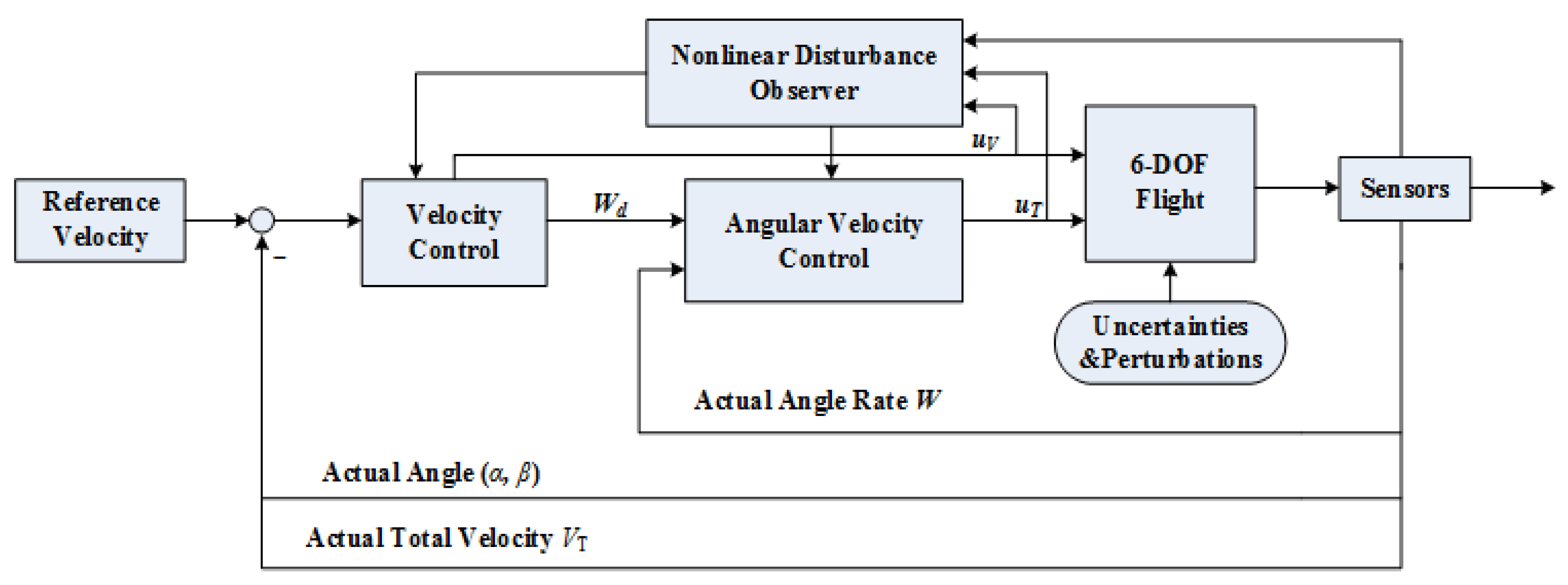
In this section, a multivariable backstepping sliding mode controller together with a nonlinear disturbance observer is proposed for the vector-coupled flight model (Eqaution (3)) so that the velocity vector $\mathit{V}$ tracks the desired vector, ${\mathit{V}}_d$. First, the control objective is established, and then the controller is derived. Figure 2 shows a schematic of the control structure.

3.1. Control Objective

Our aim is to establish a multivariable control scheme with the following properties of the flight control system.

(1) The attitude commands, ${\alpha }_d$, ${\beta }_d$, and the airspeed command of $V_d$ are tracked simultaneously by the system’s output vector $\mathit{V}$ because these commands can be transformed into a vectorial command ${\mathit{V}}_d=V_d{(\cos {\alpha }_d\cos {\beta }_d\sin {\beta }_d\sin {\alpha }_d\cos {\beta }_d)}^T$.

(2) The performance of the nominal closed-loop control system is recovered as if the lumped disturbances, $\mathit{D}1$ and $\mathit{D}2$, have been known exactly.

(3) The stability of the overall system can be guaranteed through a theoretical perspective.

3.2. Control Law Design

For convenience in deducing the control algorithm, an angular-acceleration vector is introduced as

$$\mathit{u}T={\mathit{J}}^{-1}(\mathit{M}-\mathit{W}\times \mathit{J}\mathit{W}),$$

(4)

and $\mathit{u}T$ is the control input of the system. Then, define ${\mathit{F}}_a\left(\mathit{V}\right)={\mathit{F}}_a/m$ and the dynamics can be rewritten by

$$\left\{\begin{array}{cc}\hfill \dot{\mathit{V}}& =-\mathit{W}\times \mathit{V}+\mathit{F}a(\mathit{V})+u_V{\mathit{V}}_0+\mathit{D}1,\hfill \\ \hfill \dot{\mathit{W}}& =\mathit{u}T+\mathit{D}2.\hfill \end{array}\right.$$

(5)

Remark 1.

The devices onboard to control a flight include the deflections of the aerodynamic control surfaces $\mathit{\delta }$ and the engine thrust $\mathit{T}$. The vector $\mathit{\delta }$ contains the positions of canard wings ${\delta }_c$, right elevon ${\delta }_{re}$, left elevon ${\delta }_{le}$, and rudder ${\delta }_r$, respectively. Furthermore, the engine thrust produces an acceleration of the flight along the x-axis. In this study, for the convenience of developing the vectorial controller, the control-oriental model is established and control inputs are the angular-acceleration vector ${\mathit{u}}_T={\mathit{J}}^{-1}(\mathit{M}-\mathit{W}\times (\mathit{JW}))$ and the engine thrust term $u_V$, which is assumed to be along with the velocity direction. In the angular-acceleration term, the controlled angular acceleration $\mathit{M}=q_{p}S{\left[\begin{array}{ccc}b{C}_l& c{C}_M& b{C}_n\end{array}\right]}^T$ is obtained by the deflections of the aerodynamic control surfaces, where $q_p=0.5\rho {V_T}^2$ is the dynamic pressure, ρ is the air density, $V_T$ is the velocity, S is the wing surface area, b and c are the wingspan and the mean aerodynamic chord, respectively. $C_l$, $C_M$, and $C_n$ represent the dimensionless coefficients in the moment expressions. If we can obtain the control torque vector $\mathit{M}=\mathit{J}\left({\mathit{u}}_{\mathit{T}}+\mathit{W}\times \mathit{JW}\right)$, $\mathit{\delta }$ can be obtained by $\mathit{\delta }={\mathit{B}}^{-1}\left(\mathit{J}{\mathit{u}}_{\mathit{T}}+\mathit{W}\times \mathit{JW}\right)$, where $\mathit{M}=\mathit{B}\mathit{\delta }$, and $\mathit{B}$ is the distribution matrix.

Assumption 1.

Consider the lumped disturbances of acceleration and angular acceleration, ${\mathit{D}}_1$ and ${\mathit{D}}_2$, in Equation (5), their derivatives are bounded by ${\delta }_1=\underset{t>0}{\sup }∥{\dot{\mathit{D}}}_1∥$ and ${\delta }_2=\underset{t>0}{\sup }∥{\dot{\mathit{D}}}_2∥$, where ${\delta }_1$ and ${\delta }_2$ are positive constants [4,14,27,28,29].

Remark 2.

The lumped disturbances ${\mathit{D}}_1$ and ${\mathit{D}}_2$ in Equation (5) arise from the external disturbances and un-modeled dynamics. However, they do not only depend on time, but also on the states of the flight. Considering that the flight conditions and the states may not change rapidly, we propose the above assumption [4,14,27,28,29] for the controller design in this study. In practice, because the derivatives of these uncertainties are difficult to acquire beforehand, their upper bounds, ${\delta }_1$ and ${\delta }_2$, are set relatively large to adapt with extreme flying conditions. Our future research will focus on designing an adaptive-gain controller to avoid such overshooting phenomenon.

3.2.1. Nonlinear Disturbance Observer

The uncertainties, $\mathit{D}1$ and $\mathit{D}2$, are first estimated through nonlinear disturbance observers.

Inspired by the work of Chen [30], a vectorial disturbance observer ${\widehat{\mathit{D}}}_1$ is designed to estimate the uncertain term ${\mathit{D}}_1$, which is given by

$$\left\{\begin{array}{c}\mathit{D}1={\mathit{z}}_1+{\lambda }_1{\mathit{e}}_1,\hfill \\ {\widehat{\mathit{D}}}_1={\widehat{\mathit{z}}}_1+{\lambda }_1{\mathit{e}}_1,\hfill \\ {\dot{\widehat{\mathit{z}}}}_1=-{\lambda }_1(-\mathit{W}\times \mathit{V}+{\widehat{\mathit{z}}}_1+{\lambda }_1{\mathit{e}}_{\mathbf{1}}+u_V{\mathit{V}}_0).\hfill \end{array}.\right.$$

(6)

Then, the time derivative of ${\widehat{\mathit{D}}}_1$ is

$$\begin{array}{cc}\hfill {\dot{\widehat{\mathit{D}}}}_1=& {\dot{\widehat{\mathit{z}}}}_1+{\lambda }_1{\dot{\mathit{e}}}_1\hfill \\ \hfill =& -{\lambda }_1(-\mathit{W}\times \mathit{V}+{\widehat{\mathit{z}}}_1+{\lambda }_1{\mathit{e}}_1+u_V{\mathit{V}}_0)\hfill \\ \hfill & +{\lambda }_1(-\mathit{W}\times \mathit{V}+{\mathit{D}}_1+u_V{\mathit{V}}_0)\hfill \\ \hfill =& {\lambda }_1(-{\widehat{\mathit{D}}}_1+{\mathit{D}}_1)\hfill \\ \hfill =& {\lambda }_1{\tilde{\mathit{D}}}_1.\hfill \end{array}$$

(7)

Remark 3.

The nonlinear disturbance observer’s error dynamics can be described as ${\dot{\tilde{\mathit{D}}}}_1={\dot{\mathit{D}}}_1-{\dot{\widehat{\mathit{D}}}}_1={\dot{\mathit{D}}}_1-{\lambda }_1{\tilde{\mathit{D}}}_1$, which implies ${\tilde{\mathit{D}}}_1\left(s\right)=\frac{1}{s+{\lambda }_1}{\dot{\mathit{D}}}_1\left(s\right)$, where s is the Laplace operator. Hence, the nonlinear disturbance observer’s error dynamics can be approximated by a first-order system, which can be seen as a first-order low-pass filter when the parameter ${\lambda }_1$ is selected appropriately. The nonlinear disturbance observer can handle the high-frequency noise of the disturbance differential ${\dot{\mathit{D}}}_1$ to a certain extent. This property can be verified through Case 2 in the simulation section.

Proof. 

The stability of the above nonlinear-disturbance-observer system is analyzed by introducing a Lyapunov candidate:

$$\left\{\begin{array}{cc}\hfill L_{D_1}=& 0.5{∥{\tilde{\mathit{D}}}_1∥}^2,\hfill \\ \hfill {\tilde{\mathit{D}}}_1=& {\mathit{D}}_1-{\widehat{\mathit{D}}}_1,\hfill \end{array}\right.$$

(8)

and differentiating the expression in Equation (8) yields

$$\begin{array}{cc}\hfill {\dot{L}}_{{\mathit{D}}_1}& ={{\tilde{\mathit{D}}}_1}^T{\dot{\tilde{\mathit{D}}}}_1\hfill \\ \hfill & ={{\tilde{\mathit{D}}}_1}^T({\dot{\mathit{D}}}_1-{\dot{\widehat{\mathit{D}}}}_1)\hfill \\ \hfill & ={{\tilde{\mathit{D}}}_1}^T({\dot{\mathit{D}}}_1-{\lambda }_1{\tilde{\mathit{D}}}_1)\hfill \\ \hfill & \le 0.5{∥{\tilde{\mathit{D}}}_1∥}^2+0.5{∥{\dot{\mathit{D}}}_1∥}^2-{\lambda }_1{∥{\tilde{\mathit{D}}}_1∥}^2\hfill \\ \hfill & \le -({\lambda }_1-0.5){∥{\tilde{\mathit{D}}}_1∥}^2+0.5{\delta }_1^2.\hfill \end{array}$$

(9)

It can be found, under the condition

$$\left\{\begin{array}{c}{\lambda }_1>0.5,\hfill \\ ∥{\tilde{\mathit{D}}}_1∥>\frac{{\delta }_1}{\sqrt{2({\lambda }_1-0.5)}},\hfill \end{array}\right.$$

(10)

that

$${\dot{L}}_{D_1}\le 0.$$

(11)

Therefore, the estimation error of the disturbance observer in Equation (8) is bounded by the following region

$$S({\tilde{\mathit{D}}}_1)=\left\{∥{\tilde{\mathit{D}}}_1∥\le \frac{{\delta }_1}{\sqrt{2({\lambda }_1-0.5)}}\right\}.$$

(12)

Similarly, ${\widehat{\mathit{D}}}_2$ is the disturbance-observer vector of ${\mathit{D}}_2$ which is expressed by

$$\left\{\begin{array}{c}{\mathit{D}}_2={\mathit{z}}_2+{\lambda }_2{\mathit{e}}_2,\hfill \\ {\widehat{\mathit{D}}}_2={\widehat{\mathit{z}}}_2+{\lambda }_2{\mathit{e}}_2,\hfill \\ {\dot{\widehat{\mathit{z}}}}_2=-{\lambda }_2({\mathit{u}}_T+{\widehat{\mathit{z}}}_2+{\lambda }_2{\mathit{e}}_2).\hfill \end{array}\right.$$

(13)

Moreover, the proof procedure of the above nonlinear disturbance observation of ${\mathit{D}}_2$ is akin to that of ${\mathit{D}}_1$. For the sake of space, the details are omitted herein. □

3.2.2. Multivariable Backstepping Sliding Mode Controller

Theorem 1.

Considering the control-oriented model of Equation (5), then multivariable backstepping sliding mode controller, Equations (14)–(16), can make the velocity-vector tracking error of Equation (17) be semi-globally uniformly ultimately bounded:

$$\begin{array}{cc}\hfill u_V=& k_1{({\mathit{V}}_d-\mathit{V})}^T{\mathit{V}}_0-{{\mathit{V}}_0}^T{\widehat{\mathit{D}}}_1-a{\mathit{V}}_0^T\mathit{s}({\mathit{e}}_1)-{\mathit{V}}_0^T{\mathit{F}}_a(\mathit{V}),\hfill \end{array}$$

(14)

$$\begin{array}{cc}\hfill {\mathit{W}}_d=& k_2({\mathit{V}}_d\times \mathit{V})+\frac{1}{∥\mathit{V}∥}{\mathit{V}}_{\mathbf{0}}\times {\widehat{\mathit{D}}}_1+\frac{a}{∥\mathit{V}∥}{\mathit{V}}_{\mathbf{0}}\times \mathit{s}({\mathit{e}}_1)+\frac{1}{∥\mathit{V}∥}{\mathit{V}}_{\mathbf{0}}\times {\mathit{F}}_a(\mathit{V}),\hfill \end{array}$$

(15)

$$\begin{array}{cc}\hfill {\mathit{u}}_T=& ({\mathit{V}}_d\times \mathit{V})-{\widehat{\mathit{D}}}_2-b\mathit{s}({\mathit{e}}_2)-k_3(\mathit{W}-{\mathit{W}}_d)+{\mathit{d}}_{\dot{w}},\hfill \end{array}$$

(16)

where

$${\mathit{e}}_1=\mathit{V}-{\mathit{V}}_d,$$

(17)

$${\mathit{e}}_2=\mathit{W}-{\mathit{W}}_d,$$

(18)

$$\mathit{s}({\mathit{e}}_1)=\frac{{\mathit{e}}_1}{∥{\mathit{e}}_1∥+{\epsilon }_1},$$

(19)

$$\mathit{s}({\mathit{e}}_2)=\frac{{\mathit{e}}_2}{∥{\mathit{e}}_2∥+{\epsilon }_2},$$

(20)

$$a>\frac{{\delta }_1}{\sqrt{2({\lambda }_1-0.5)}},$$

(21)

$$b>\frac{{\delta }_2}{\sqrt{2({\lambda }_2-0.5)}},$$

(22)

$$\tau {\dot{\mathit{d}}}_{\dot{w}}+{\mathit{d}}_{\dot{w}}={\mathit{W}}_d,\tau >0.$$

(23)

${\widehat{\mathit{D}}}_1$ and ${\widehat{\mathit{D}}}_2$ are the observers of $\mathit{D}1$ and $\mathit{D}2$, respectively, which are depicted by

$$\left\{\begin{array}{c}\mathit{D}1={\mathit{z}}_1+{\lambda }_1{\mathit{e}}_1,\hfill \\ {\widehat{\mathit{D}}}_1={\widehat{\mathit{z}}}_1+{\lambda }_1{\mathit{e}}_1,\hfill \\ {\dot{\widehat{\mathit{z}}}}_1=-{\lambda }_1(-\mathit{W}\times \mathit{V}+{\widehat{\mathit{z}}}_1+{\lambda }_1{\mathit{e}}_{\mathbf{1}}+u_V{\mathit{V}}_{\mathbf{0}}),\hfill \end{array}\right.$$

(24)

$$\left\{\begin{array}{c}{\mathit{D}}_2={\mathit{z}}_2+{\lambda }_2{\mathit{e}}_2,\hfill \\ {\widehat{\mathit{D}}}_2={\widehat{\mathit{z}}}_2+{\lambda }_2{\mathit{e}}_2,\hfill \\ {\dot{\widehat{\mathit{z}}}}_2=-{\lambda }_2({\widehat{\mathit{z}}}_2+{\lambda }_2{\mathit{e}}_2+{\mathit{u}}_T),\hfill \end{array}\right.$$

(25)

$$\left\{\begin{array}{c}{\lambda }_1>0.5,\hfill \\ {\lambda }_2>0.5.\hfill \end{array}\right.$$

(26)

Proof of Theorem 1. 

Theorem 1 can be proved by the following two steps.

Step 1. Firstly, the angular velocity $\mathit{W}$ and $u_V$ are viewed as control input variables to control the velocity vector $\mathit{V}$ tracking the given command ${\mathit{V}}_d$.

The error ${\mathit{e}}_1$ is defined as the expected sliding mode surface, and a Lyapunov candidate is selected as:

$$\left\{\begin{array}{cc}\hfill L_1& =0.5{\mathit{e}}_1^2,\hfill \\ \hfill {\mathit{e}}_1& =\mathit{V}-{\mathit{V}}_d,\hfill \end{array}\right.$$

(27)

and introduce the virtual control term ${\mathit{W}}_d$ as the expectation of the angular velocity $\mathit{W}$.

Differentiating the first equation of Equation (27) yields

$${\dot{L}}_1={(\mathit{V}-{\mathit{V}}_d)}^T(-\mathit{W}\times \mathit{V}+{\mathit{F}}_a(\mathit{V})+u_V{\mathit{V}}_0+{\mathit{D}}_1).$$

(28)

We construct the control input $u_V$ and virtual angular-velocity control term ${\mathit{W}}_d$ as

$$\left\{\begin{array}{cc}\hfill u_{{}_V}=& {\overline{u}}_V-{\mathit{V}}_0^T{\widehat{\mathit{D}}}_1-a{\mathit{V}}_0^{T}s({\mathit{e}}_1)-{{\mathit{V}}_{\mathbf{0}}}^T{\mathit{F}}_a(\mathit{V}),\hfill \\ \hfill {\mathit{W}}_d=& \overline{\mathit{W}}+\frac{1}{∥\mathit{V}∥}{\mathit{V}}_0\times {\widehat{\mathit{D}}}_1+\frac{a}{∥\mathit{V}∥}{\mathit{V}}_0\times \mathit{s}({\mathit{e}}_1)+\frac{1}{∥\mathit{V}∥}{\mathit{V}}_0\times {\mathit{F}}_a(\mathit{V}),\hfill \end{array}\right.$$

(29)

where ${\overline{u}}_V$ and $\overline{\mathit{W}}$ are parts of $u_V$ and ${\mathit{W}}_d$, respectively, and they will be designed in the following part.

To eliminate the chattering caused by the sign function, a continuous saturation function is employed to replace it, which can be described as

$$s({\mathit{e}}_1)=\frac{{\mathit{e}}_1}{∥{\mathit{e}}_1∥+{\epsilon }_1},$$

(30)

where ${\epsilon }_1$ is a small positive constant.

For an arbitrary vector $\mathit{\chi }$ and a unit vector ${\mathit{V}}_0$, the relationship below exists

$$\mathit{\chi }={\mathit{V}}_0^T·\mathit{\chi }·{\mathit{V}}_0+{\mathit{V}}_0\times \mathit{\chi }\times {\mathit{V}}_0.$$

(31)

Then,

$$\left\{\begin{array}{cc}\hfill {\widehat{\mathit{D}}}_1=& \left[{\mathit{V}}_0^T{\widehat{\mathit{D}}}_1\right]{\mathit{V}}_0+\frac{1}{∥\mathit{V}∥}[{\mathit{V}}_0\times {\widehat{\mathit{D}}}_1]\times \mathit{V},\hfill \\ \hfill \mathit{s}({\mathit{e}}_1)=& \left[{\mathit{V}}_0^T\mathit{s}({\mathit{e}}_1)\right]{\mathit{V}}_0+\frac{1}{∥\mathit{V}∥}[{\mathit{V}}_0\times \mathit{s}({\mathit{e}}_1)]\times \mathit{V},\hfill \\ \hfill {\mathit{F}}_a(\mathit{V})=& \left[{\mathit{V}}_0^T{\mathit{F}}_a(\mathit{V})\right]{\mathit{V}}_0+\frac{1}{∥\mathit{V}∥}[{\mathit{V}}_0\times {\mathit{F}}_a(\mathit{V})]\times \mathit{V}.\hfill \end{array}\right.$$

(32)

Substituting Equations (29), (30) and (32) into Equation (28) leads to

$$\begin{array}{cc}\hfill {\dot{L}}_1=& {(\mathit{V}-{\mathit{V}}_d)}^T\{-\overline{\mathit{W}}\times \mathit{V}+{\mathit{F}}_a(\mathit{V})+{\mathit{D}}_1+{\overline{u}}_V{\mathit{V}}_0\hfill \\ \hfill & -({\mathit{V}}_0^T{\widehat{\mathit{D}}}_1)\widehat{\mathit{V}}-({\mathit{V}}_0^T{\mathit{F}}_a(\mathit{V})){\mathit{V}}_0-\frac{1}{∥\mathit{V}∥}[{\mathit{V}}_0\times {\widehat{\mathit{D}}}_1]\times \mathit{V}\hfill \\ \hfill & -\frac{1}{∥\mathit{V}∥}[{\mathit{V}}_0\times {\mathit{F}}_a(\mathit{V})]\times \mathit{V}-a\left[({\mathit{V}}_0^T\mathit{s}({\mathit{e}}_1))\widehat{\mathit{V}}\right]\hfill \\ \hfill & -a\frac{1}{∥\mathit{V}∥}[{\mathit{V}}_0\times \mathit{s}({\mathit{e}}_1)]\times \mathit{V}\}\hfill \\ \hfill =& {(\mathit{V}-{\mathit{V}}_d)}^T(-\overline{\mathit{W}}\times \mathit{V}+{\overline{u}}_V{\mathit{V}}_0+{\mathit{D}}_1-{\widehat{\mathit{D}}}_1-a\mathit{s}({\mathit{e}}_1))\hfill \\ \hfill =& {(\mathit{V}-{\mathit{V}}_d)}^T(-\overline{\mathit{W}}\times \mathit{V}+{\overline{u}}_V{\mathit{V}}_0+{\tilde{\mathit{D}}}_1-a\mathit{s}({\mathit{e}}_1)).\hfill \end{array}$$

(33)

We then select $\overline{\mathit{W}}$ and ${\overline{u}}_V$ to make ${\dot{L}}_1$ negative

$$\begin{array}{cc}\hfill {\dot{L}}_1=& {(\mathit{V}-{\mathit{V}}_d)}^T(-\overline{\mathit{W}}\times \mathit{V}+{\overline{u}}_V{\mathit{V}}_0+{\tilde{\mathit{D}}}_1-a\mathit{s}({\mathit{e}}_1))\hfill \\ \hfill =& {(\mathit{V}-{\mathit{V}}_d)}^T(-\overline{\mathit{W}}\times \mathit{V}+{\overline{u}}_V{\mathit{V}}_0)+{\mathit{e}}_1^T{\tilde{\mathit{D}}}_1-a{\mathit{e}}_1^T\mathit{s}({\mathit{e}}_1)\hfill \\ \hfill \le & {{\mathit{V}}_d}^T(\overline{\mathit{W}}\times \mathit{V})+{\overline{u}}_V{(\mathit{V}-{\mathit{V}}_d)}^T{\mathit{V}}_0\hfill \\ \hfill & +\frac{{\delta }_1}{\sqrt{2({\lambda }_1-0.5)}}\sum _{i=1}^3∥{\mathit{e}}_{1i}∥-a{\mathit{e}}_1^T\mathit{s}({\mathit{e}}_1).\hfill \end{array}$$

(34)

It can be found, under the condition

$$\left\{\begin{array}{cc}\hfill {\overline{u}}_V& =k_1{({\mathit{V}}_d-\mathit{V})}^T{\mathit{V}}_0,\hfill \\ \hfill \overline{\mathit{W}}& =k_2({\mathit{V}}_d\times \mathit{V}),\hfill \end{array}\right.$$

(35)

that

$$\begin{array}{cc}\hfill {\dot{L}}_1\le & -k_1{({(\mathit{V}-{\mathit{V}}_d)}^T\widehat{\mathit{V}})}^2-k_2{∥{\mathit{V}}_d\times \mathit{V}∥}^2\hfill \\ \hfill & +\frac{{\delta }_1}{\sqrt{2({\lambda }_1-0.5)}}∥{\mathit{e}}_1∥-a{\mathit{e}}_1^T\frac{{\mathit{e}}_1}{∥{\mathit{e}}_1∥+{\epsilon }_1}\hfill \\ \hfill \le & -2k_1{L}_1+\frac{{\delta }_1}{\sqrt{2({\lambda }_1-0.5)}}∥{\mathit{e}}_1∥\hfill \\ \hfill & -a{\mathit{e}}_1^T\frac{{\mathit{e}}_1}{∥{\mathit{e}}_1∥+{\epsilon }_1}+a\frac{{\epsilon }_1^2}{∥{\mathit{e}}_1∥+{\epsilon }_1}\hfill \\ \hfill =& -2k_1{L}_1+\frac{{\delta }_1}{\sqrt{2({\lambda }_1-0.5)}}∥{\mathit{e}}_1∥-a∥{\mathit{e}}_1∥+a{\epsilon }_1\hfill \\ \hfill =& -2k_1{L}_1+(\frac{{\delta }_1}{\sqrt{2({\lambda }_1-0.5)}}-a)∥{\mathit{e}}_1∥+a{\epsilon }_1.\hfill \end{array}$$

(36)

As long as

$$a>\frac{{\delta }_1}{\sqrt{2({\lambda }_1-0.5)}},$$

(37)

one can obtain

$${\dot{L}}_1\le -2k_1{L}_1+a{\epsilon }_1.$$

(38)

By solving the differential inequality (Equation (38)), we have

$$0\le L_1\le \frac{a{\epsilon }_1}{2k_1}+(L_1(0)-\frac{a{\epsilon }_1}{2k_1})e^{-2k_{1}t},\forall t\ge 0.$$

(39)

We can conclude that $L_1$ is bounded by $\frac{a{\epsilon }_1}{2k_1}$, i.e., $0\le L_1\le \frac{a{\epsilon }_1}{2k_1},t\to \infty$.

In summary, the control inputs

$$\left\{\begin{array}{cc}\hfill u_{{}_V}=& k_1{({\mathit{V}}_d-\mathit{V})}^T{\mathit{V}}_0-{\mathit{V}}_0^T{\widehat{\mathit{D}}}_1-a{\mathit{V}}_0^T\mathit{s}({\mathit{e}}_1)-{\mathit{V}}_0^T{\mathit{F}}_a(\mathit{V}),\hfill \\ \hfill {\mathit{W}}_d=& k_2({\mathit{V}}_d\times \mathit{V})+\frac{1}{∥\mathit{V}∥}{\mathit{V}}_0\times {\widehat{\mathit{D}}}_1+\frac{a}{∥\mathit{V}∥}{\mathit{V}}_0\times \mathit{s}({\mathit{e}}_1)+\frac{1}{∥\mathit{V}∥}{\mathit{V}}_0\times {\mathit{F}}_a(\mathit{V}),\hfill \end{array}\right.$$

(40)

along with the Lyapunov function $L_1$, thus ensuring that $\mathit{V}$ converges to an arbitrary small neighborhood around the desired ${\mathit{V}}_d$ if $u_V$ and $\mathit{W}$ can achieve the control values described in Equation (40).

Step 2. Second, the angular acceleration ${\mathit{u}}_T$ is the control input to maintain the angular-velocity vector $\mathit{W}$ tracking the desired virtual angular-velocity vector ${\mathit{W}}_d$.

We define the error ${\mathit{e}}_2$ as the expectedu sliding-mode-surface vector, which represents the tracking error of the angular velocity

$${\mathit{e}}_2=\mathit{W}-{\mathit{W}}_d.$$

(41)

Then, the dynamics can be rewritten as

$$\begin{array}{c}\hfill \dot{\mathit{V}}=-{\mathit{W}}_d\times \mathit{V}+\mathit{F}a(\mathit{V})+u_V{\mathit{V}}_0-{\mathit{e}}_2\times \mathit{V}+{\mathit{D}}_1.\end{array}$$

(42)

The time derivative of ${\mathit{e}}_2$ is

$${\dot{\mathit{e}}}_2={\mathit{u}}_T-{\mathit{d}}_{\dot{w}}+{\mathit{D}}_2,$$

(43)

where

$$\tau {\dot{\mathit{d}}}_{\dot{w}}+{\mathit{d}}_{\dot{w}}={\mathit{W}}_d,\tau >0.$$

(44)

The control algorithm is proposed by

$${\mathit{u}}_T=({\mathit{V}}_d\times \mathit{V})-{\widehat{\mathit{D}}}_2-b\mathit{s}({\mathit{e}}_2)-k_3(\mathit{W}-{\mathit{W}}_d)+{\mathit{d}}_{\dot{w}},$$

(45)

where

$$\mathit{s}({\mathit{e}}_2)=\frac{{\mathit{e}}_2}{∥{\mathit{e}}_2∥+{\epsilon }_2},$$

(46)

and ${\epsilon }_2$ is a small positive value.

From the above, a Lyapunov candidate is chosen by:

$$\begin{array}{cc}\hfill L=& L_1+L_2+L_{D_1}+L_{D_2}\hfill \\ \hfill =& \frac{1}{2}{\mathit{e}}_1^2+\frac{1}{2}{\mathit{e}}_2^2+\frac{1}{2}{\tilde{\mathit{D}}}_1^2+\frac{1}{2}{\tilde{\mathit{D}}}_2^2.\hfill \end{array}$$

(47)

Then, the time derivative of (Equation (47)) is

$$\begin{array}{cc}\hfill \dot{L}=& {\mathit{e}}_1^T{\dot{\mathit{e}}}_1+{\mathit{e}}_2^T{\dot{\mathit{e}}}_2+{\tilde{\mathit{D}}}_1^T{\dot{\tilde{\mathit{D}}}}_1+{\tilde{\mathit{D}}}_2^T{\dot{\tilde{\mathit{D}}}}_2\hfill \\ \hfill \le & -k_1{({(\mathit{V}-{\mathit{V}}_d)}^T\widehat{\mathit{V}})}^2-k_2{∥{\mathit{V}}_d\times \mathit{V}∥}^2\hfill \\ \hfill & -\left(a-\frac{{\delta }_1}{\sqrt{2({\lambda }_1-0.5)}}\right)\sum _{i=1}^3\left|e_{1i}\right|\hfill \\ \hfill & +\left(\frac{{\delta }_2}{\sqrt{2({\lambda }_2-0.5)}}-b\right)\sum _{i=1}^3\left|e_{2i}\right|\hfill \\ \hfill & -k_3{\mathit{e}}_2^2-({\lambda }_1-0.5){∥{\tilde{\mathit{D}}}_1∥}^2+0.5{\delta }_1^2\hfill \\ \hfill & -({\lambda }_2-0.5){∥{\tilde{\mathit{D}}}_2∥}^2+0.5{\delta }_2^2+a{\epsilon }_1+b{\epsilon }_2\hfill \\ \hfill \le & -k_1{\mathit{e}}_1^2-k_3{\mathit{e}}_2^2-({\lambda }_1-0.5){∥{\tilde{\mathit{D}}}_1∥}^2\hfill \\ \hfill & -({\lambda }_2-0.5){∥{\tilde{\mathit{D}}}_2∥}^2+(0.5{\delta }_1^2+0.5{\delta }_2^2+a{\epsilon }_1+b{\epsilon }_2)\hfill \\ \hfill \le & -2\xi (\frac{1}{2}{\mathit{e}}_1^2+\frac{1}{2}{\mathit{e}}_2^2+\frac{1}{2}{\tilde{\mathit{D}}}_1^2+\frac{1}{2}{\tilde{\mathit{D}}}_2^2)+\eta \hfill \\ \hfill =& -2\xi L+\eta ,\hfill \end{array}$$

(48)

where

$$\xi =\min \left(k_1,k_3,{\lambda }_1-0.5,{\lambda }_2-0.5\right),$$

(49)

$$\eta =0.5({\delta }_1^2+{\delta }_2^2)+a{\epsilon }_1+b{\epsilon }_2.$$

(50)

By solving the differential equation of (Equation (48)), we can obtain

$$0\le L\le \frac{\eta }{2\xi }+(L(0)-\frac{\eta }{2\xi })e^{-2\xi t},\forall t\ge 0.$$

(51)

We can conclude that L is bounded by $\frac{\eta }{2\xi }$, i.e., $0\le L\le \frac{\eta }{2\xi },t\to \infty$.

Then, it can be deduced that ${\mathit{e}}_1$, ${\mathit{e}}_2$, ${\tilde{\mathit{D}}}_1$, and ${\tilde{\mathit{D}}}_2$ are all semi-globally uniformly ultimately bounded:

$$∥{\mathit{e}}_1∥\le \sqrt{\frac{\eta }{\xi }+2L(0)},\forall t\ge 0$$

(52)

and

$$∥{\mathit{e}}_1∥\le \sqrt{\frac{\eta }{\xi }},t\to \infty .$$

(53)

We can obtain

$$\left|e_{1i}\right|\le \sqrt{\frac{\eta }{\xi }+2L(0)},\forall t\ge 0,i=1,2,3$$

(54)

and

$$\left|e_{1i}\right|\le \sqrt{\frac{\eta }{\xi }},t\to \infty ,i=1,2,3.$$

(55)

From inequalities Equation (52) to Equation (55), it can be concluded that the respective tracking errors of airspeed ($V_T$), AOA ($\alpha$), and sideslip angle ($\beta$) can converge to arbitrary small domains of the origin. In addition, the designed controller can guarantee that the vectorial sliding manifold practically converges to the origin. □

Remark 4.

${\mathit{d}}_{\dot{w}}$ is the derivative vector of the virtual angular-velocity controller ${\mathit{W}}_d$. However, ${\mathit{W}}_d$ may not be practically differentiable owing to undifferentiable noise or disturbance. To solve this problem, this study is inspired by the work of [31,32]; we adopt the low-pass filter technique in a vectorial manner.

Remark 5.

Flight control law interpretation: the different terms in the control algorithm, Equations (14)–(16) can be interpreted as follows:

$$\begin{array}{cccc}\hfill u_V=& k_1{({\mathit{V}}_d-\mathit{V})}^T{\mathit{V}}_0\hfill & \hfill & controlof∥\mathit{V}∥\hfill \\ \hfill & -{{\mathit{V}}_0}^T{\widehat{\mathit{D}}}_1-a{\mathit{V}}_0^T\mathit{s}({\mathit{e}}_1)\hfill & \hfill & cancelof{\mathit{D}}_1\hfill \\ \hfill & -{{\mathit{V}}_0}^T{\mathit{F}}_a(\mathit{V})\hfill & \hfill & cancelof{\mathit{F}}_a(\mathit{V}),\hfill \end{array}$$

(56)

$$\begin{array}{cccc}\hfill {\mathit{W}}_{{}^d}=& k_2({\mathit{V}}_d\times \mathit{V})\hfill & \hfill & controlof{\mathit{V}}^{\prime }sdirection\hfill \\ \hfill & +\frac{1}{∥\mathit{V}∥}{\mathit{V}}_0\times {\widehat{\mathit{D}}}_1+\frac{a}{∥\mathit{V}∥}{\mathit{V}}_0\times \mathit{s}({\mathit{e}}_1)\hfill & \hfill & cancelof{\mathit{D}}_1\hfill \\ \hfill & +\frac{1}{∥\mathit{V}∥}{\mathit{V}}_0\times {\mathit{F}}_a(\mathit{V})\hfill & \hfill & cancelof{\mathit{F}}_a(\mathit{V}),\hfill \end{array}$$

(57)

$$\begin{array}{cccc}\hfill {\mathit{u}}_T=& ({\mathit{V}}_d\times \mathit{V})\hfill & \hfill & controlof{\mathit{V}}^{\prime }sdirection\hfill \\ \hfill & -k_3(\mathit{W}-{\mathit{W}}_d)\hfill & \hfill & controlof\mathit{W}\hfill \\ \hfill & -{\widehat{\mathit{D}}}_2-b\mathit{s}({\mathit{e}}_2)\hfill & \hfill & cancelof{\mathit{D}}_2\hfill \\ \hfill & +{\mathit{d}}_{\dot{w}}\hfill & \hfill & cancelof\frac{d{\mathit{W}}_d}{dt}.\hfill \end{array}$$

(58)

From the interpretation of Equations (56)–(58), the developed combined control scheme has a symmetry structure between $u_V$ and ${\mathit{W}}_{{}^d}$, which is concise and aesthetically appealing compared with the traditional control structures that decoupled the dynamic equations and used a collection of single variables [12,16,17,18,19]. Moreover, each term is meaningful, and this feature is significant as the control parameters can be adjusted in each term directively.

Remark 6.

The developed multivariable backstepping and sliding mode controller with nonlinear disturbance observer is deduced directly on the vector-coupled dynamics. In addition, this study deals with the cross-coupling by vector operations, including inner product algorithm and cross multiply algorithm, which takes the interaction between the state variables automatically and directly into account. Unlike similar works [12,16,17,18,19], the developed controller not only avoids solving complex matrix equations and treating inverse matrixes, but also fully realizes vector-coupled control.

4. Simulations

The effectiveness and robustness of the proposed combined multivariable backstepping sliding mode controller is verified by using the ADMIRE aircraft model [33]. The deflections of the aerodynamic control surfaces $\mathit{\delta }$ in the ADMIRE aircraft model include the canard wings, the right and left elevons, and the rudder. These control inputs are limited by ${\delta }_c\in \left[-{55}^{\circ },{25}^{\circ }\right]$, ${\delta }_{re}\in \left[-{25}^{\circ },{25}^{\circ }\right]$, ${\delta }_{le}\in \left[-{25}^{\circ },{25}^{\circ }\right]$, and ${\delta }_r\in \left[-{30}^{\circ },{30}^{\circ }\right]$, respectively. They are listed on

Table 1. Control input units and maximum values.

Control	Unit	Min.	Max.	Rate Limit
Canard wings	deg	−55	25	±50 deg/s
Right elevon	deg	−25	25	±50 deg/s
Left elevon	deg	−25	25	±50 deg/s
Rudder	deg	−30	30	±50 deg/s

. Furthermore, $m=9100$ kg and maximum engine thrust is set with 100 kN, which means the engine thrust control input term $u_V\in [0,10.99]$ m/s${}^2$. The initial values of the simulation are chosen as $V_0=80$ m/s, $H_0=3000$ m, ${\alpha }_0=0$ deg, ${\beta }_0=0$ deg, $p_0=q_0=r_0=0$ rad/s. The gains of the controller are selected as $k_1=0.2$, $k_2=0.005$, $k_3=0.01$, $a=10$, $b=20$, ${\lambda }_1=5$ and ${\lambda }_2=20$. The command signal is given by

$${\mathit{V}}_d=V_T^{ref}{\left(\begin{array}{c}\cos {\alpha }^{ref}\cos {\beta }^{ref},\sin {\beta }^{ref},\sin {\alpha }^{ref}\cos {\beta }^{ref}\end{array}\right)}^T.$$

(59)

The disturbances ${\mathit{D}}_1$ and ${\mathit{D}}_2$ are selected as

$${\mathit{D}}_1=\left[\begin{array}{c}-2.1-0.1\cos \left(0.5t\right)-0.1\sin \left(t\right)\\ -1.2-0.3\sin \left(0.5t\right)+0.1\sin \left(t\right)\\ 1.1+0.2\cos \left(0.5t\right)+0.1\sin \left(t\right)\end{array}\right]\left(\mathrm{m}/{\mathrm{s}}^2\right),$$

(60)

$${\mathit{D}}_2=\left[\begin{array}{c}-0.1\cos \left(0.5t\right)-0.1\sin \left(t\right)\\ 0.1-0.3\sin \left(0.5t\right)-0.1\sin \left(t\right)\\ 0.1\cos \left(2t\right)-0.1\sin \left(t\right)\end{array}\right]\left(\mathrm{rad}/{\mathrm{s}}^2\right).$$

(61)

To illustrate the effectiveness and robustness of the proposed vectorial controller, three cases are selected. The sampling step is 0.001 s, and the simulation results are shown in Figure 3, Figure 4, Figure 5, Figure 6, Figure 7, Figure 8, Figure 9, Figure 10, Figure 11 and Figure 12. To avoid the abrupt control input change, the command passes through the filter with desired flying qualities:

$$\frac{x_r\left(s\right)}{x_c\left(s\right)}=\frac{w_n^2}{s^2+2{\xi }_n{w}_n+w_n^2},$$

(62)

where $w_n=3\mathrm{rad}/\mathrm{s}$, and ${\xi }_n=1$.

4.1. Effectiveness of the Proposed Controller

Case 1.

To illustrate the effectiveness of the proposed controller, the commands were given as follows:

$$\left\{\begin{array}{c}{V}_{{}_T}^{ref}=80m/s,{\alpha }^{ref}={10}^{\circ },{\beta }^{ref}=0^{\circ },0<t\le 10s,\hfill \\ V_{{}_T}^{ref}=90m/s,{\alpha }^{ref}={-2}^{\circ },{\beta }^{ref}=4^{\circ },10<t\le 20s.\hfill \end{array}\right.$$

(63)

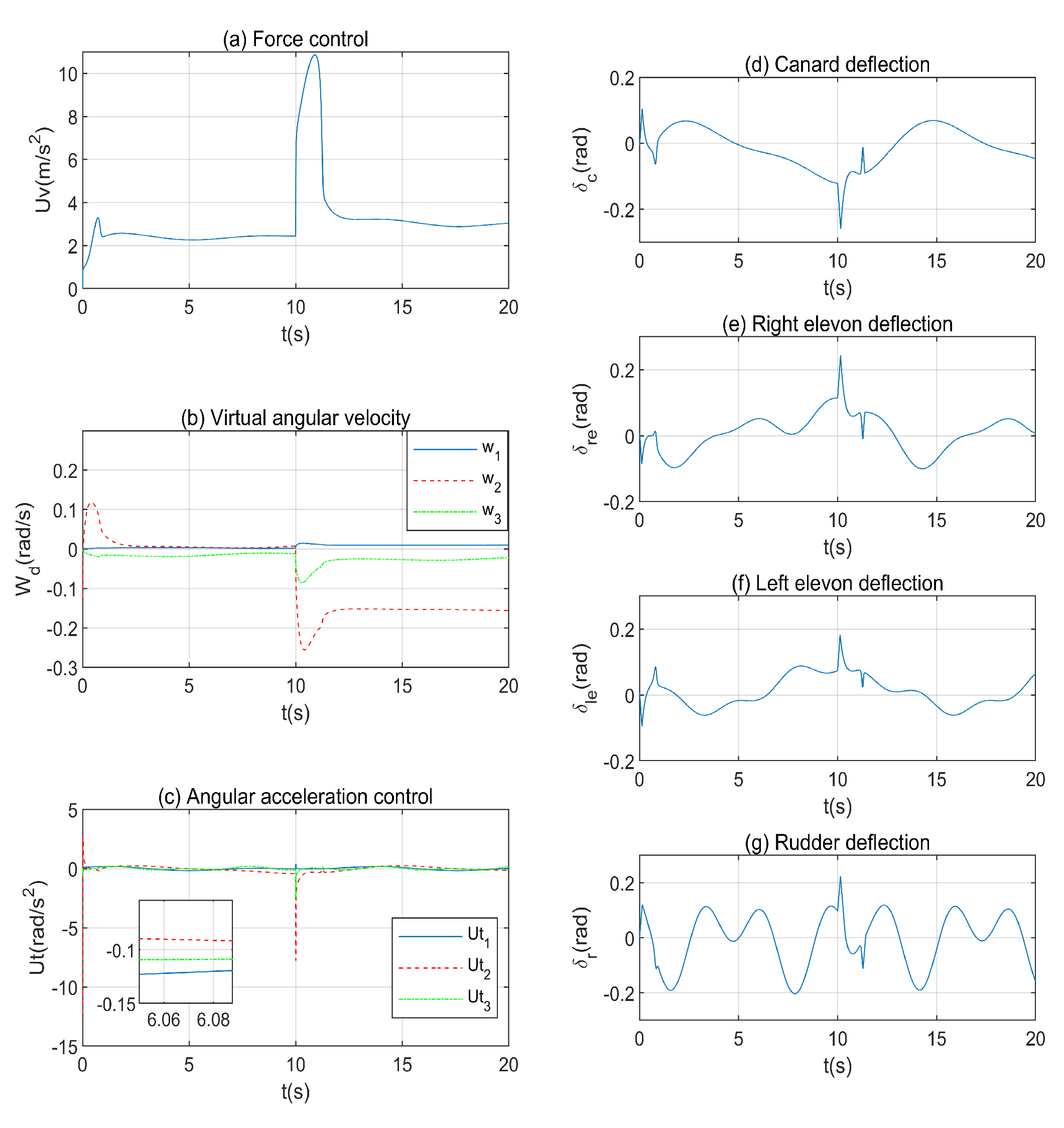
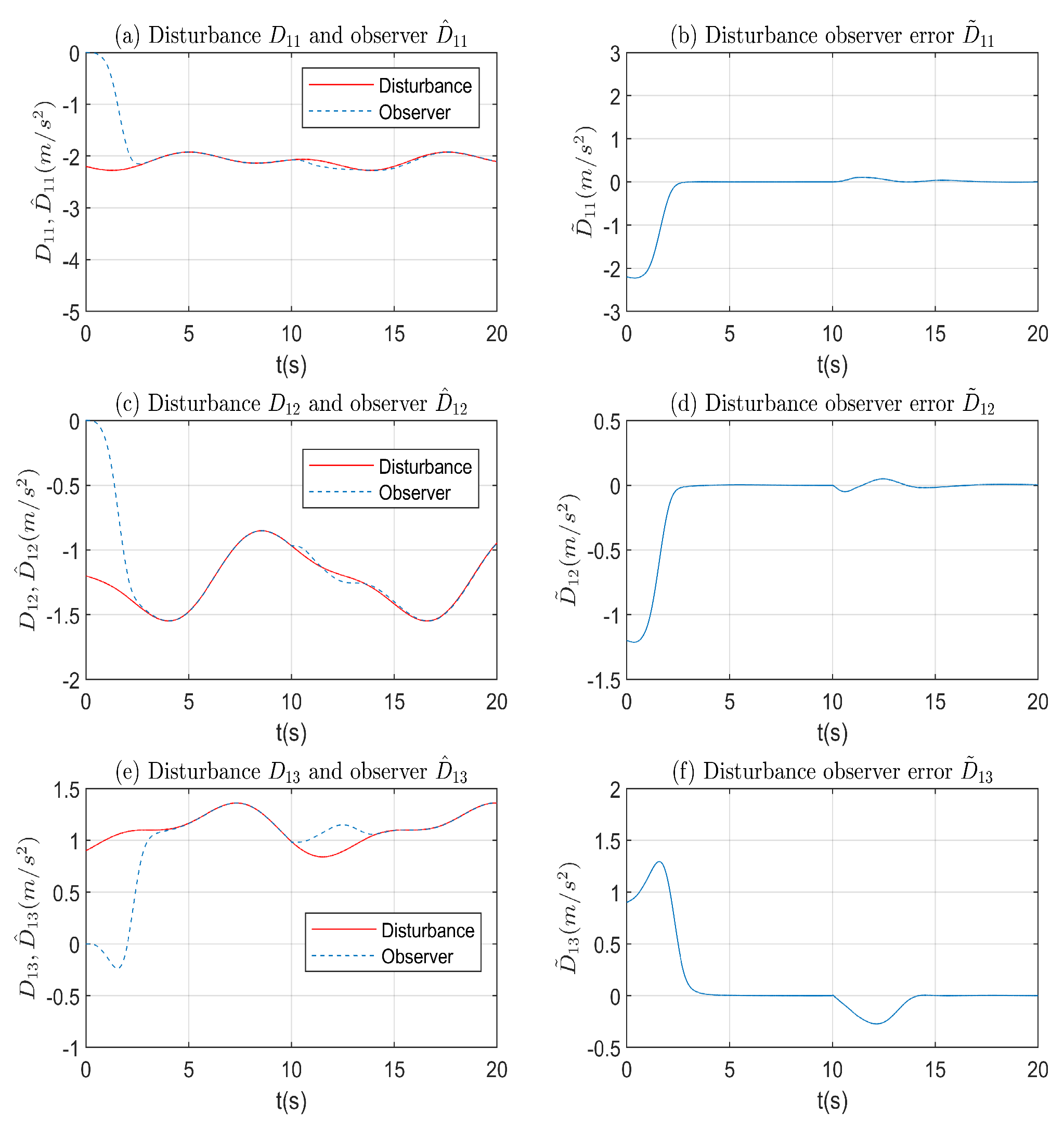
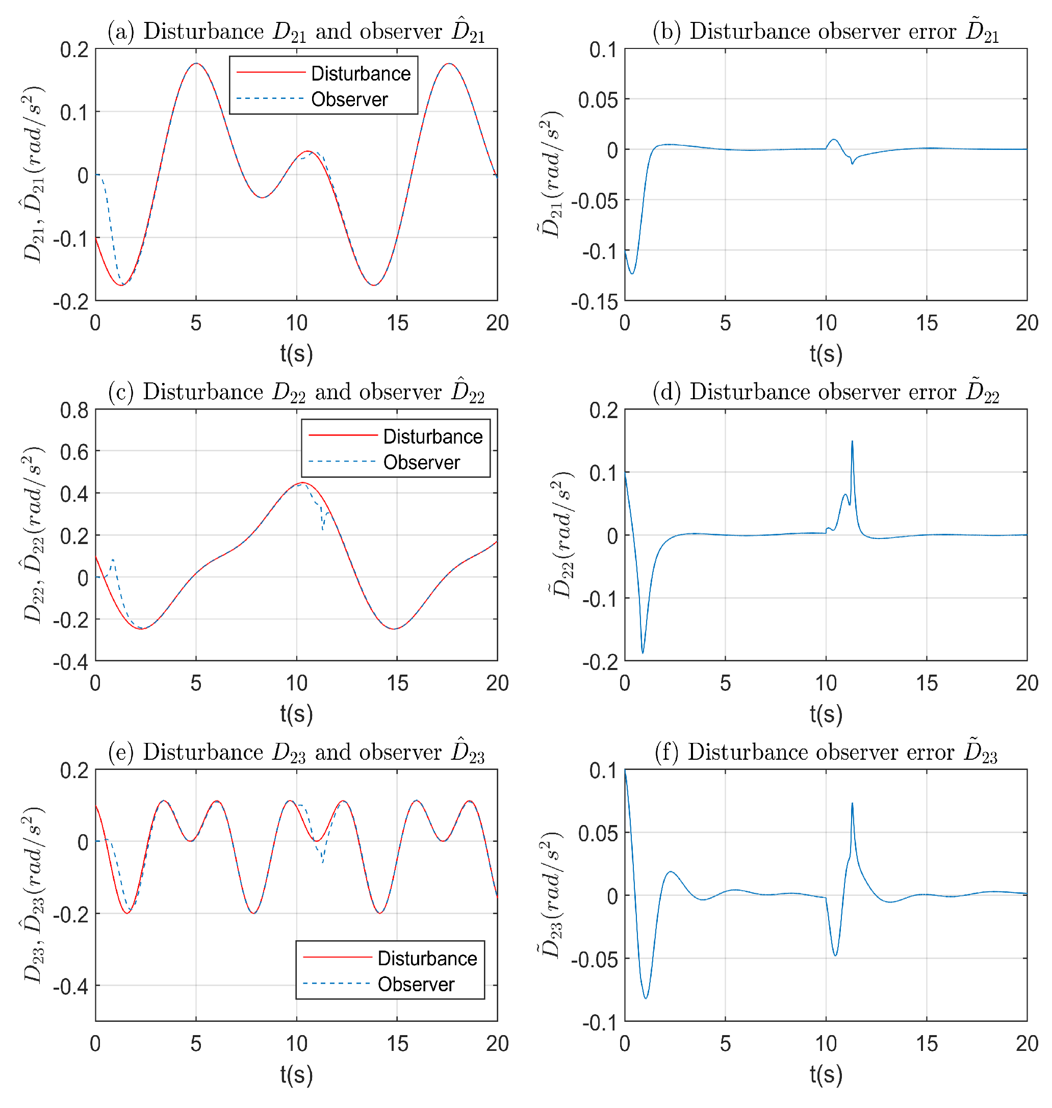
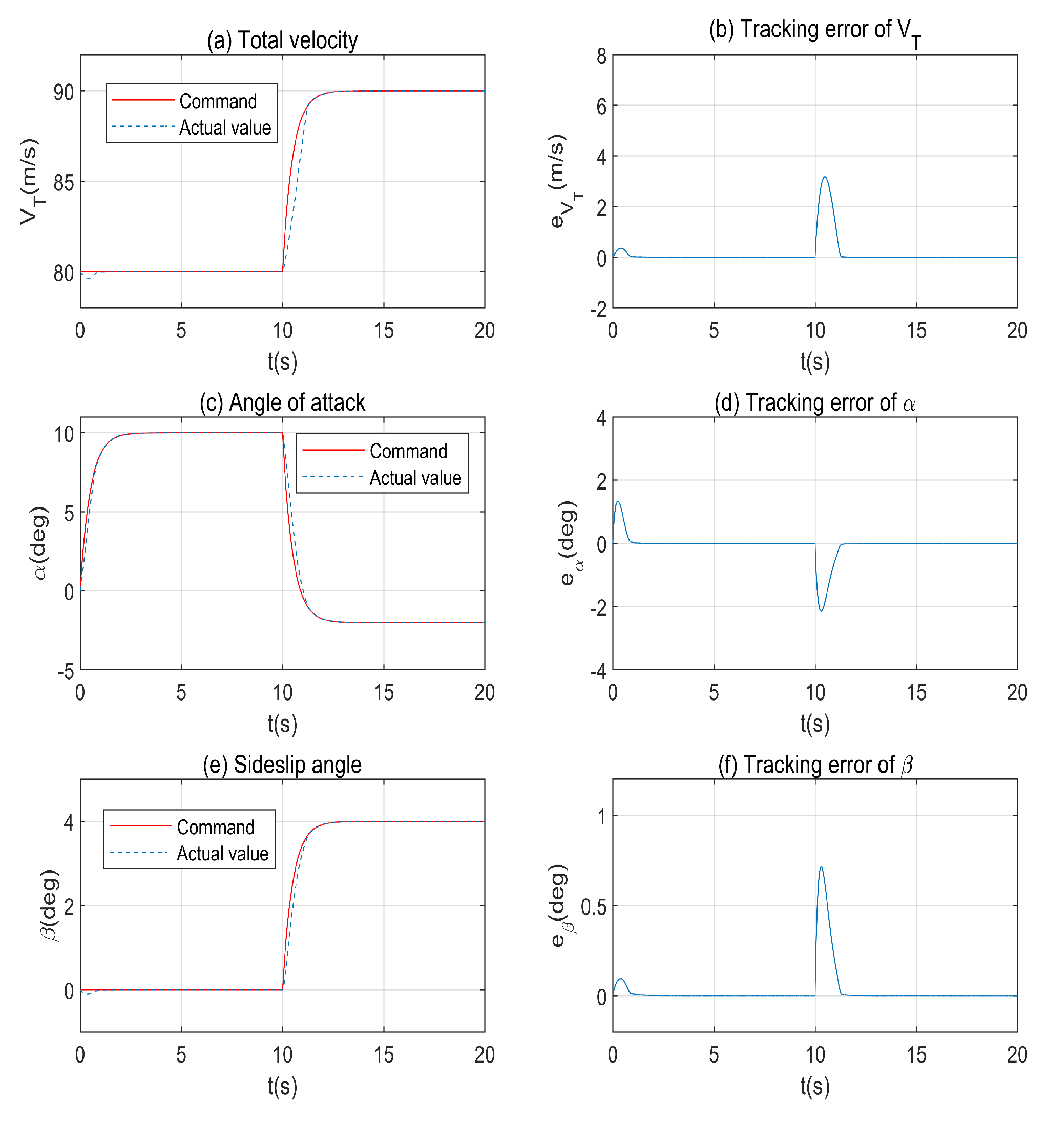
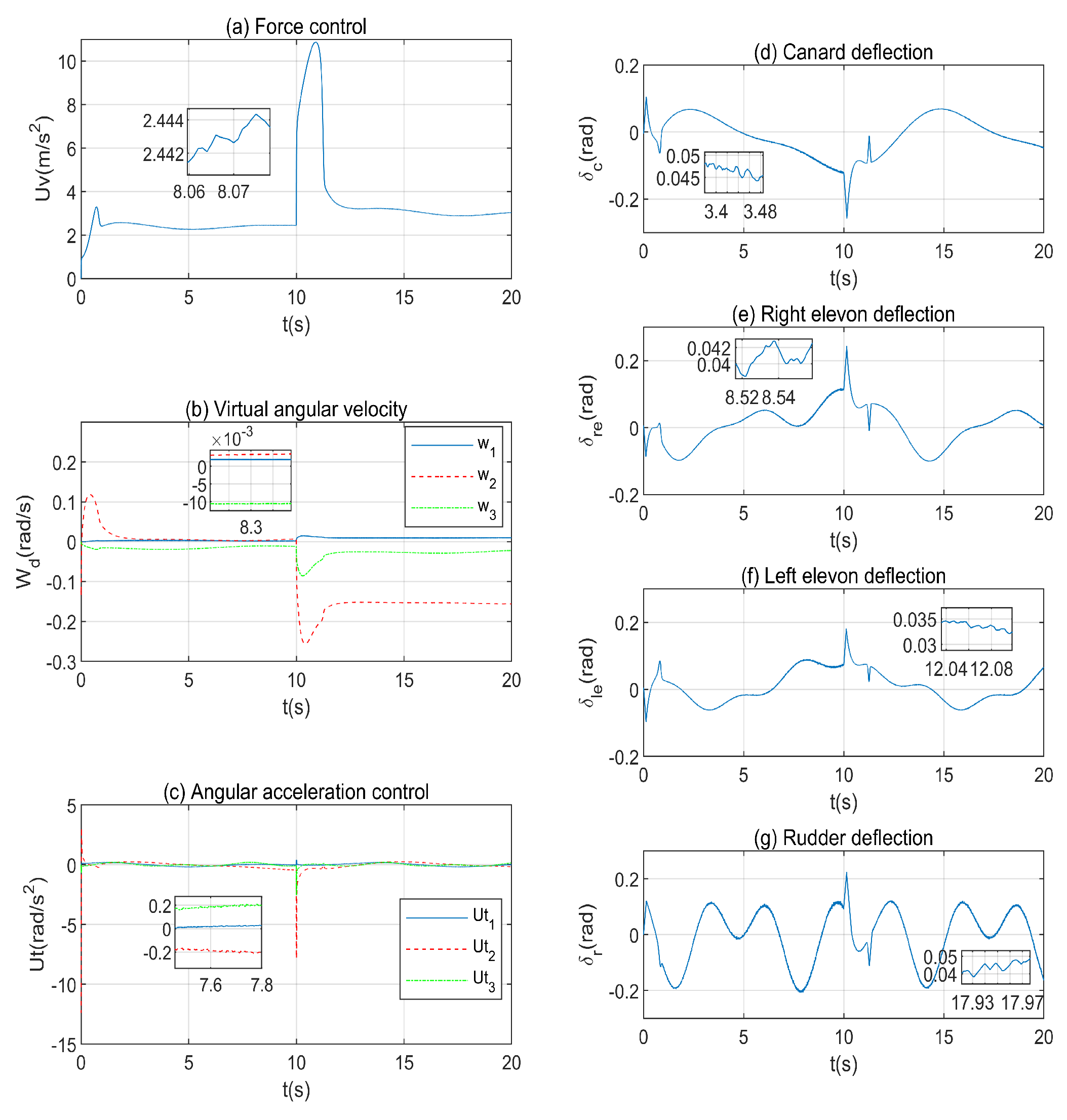
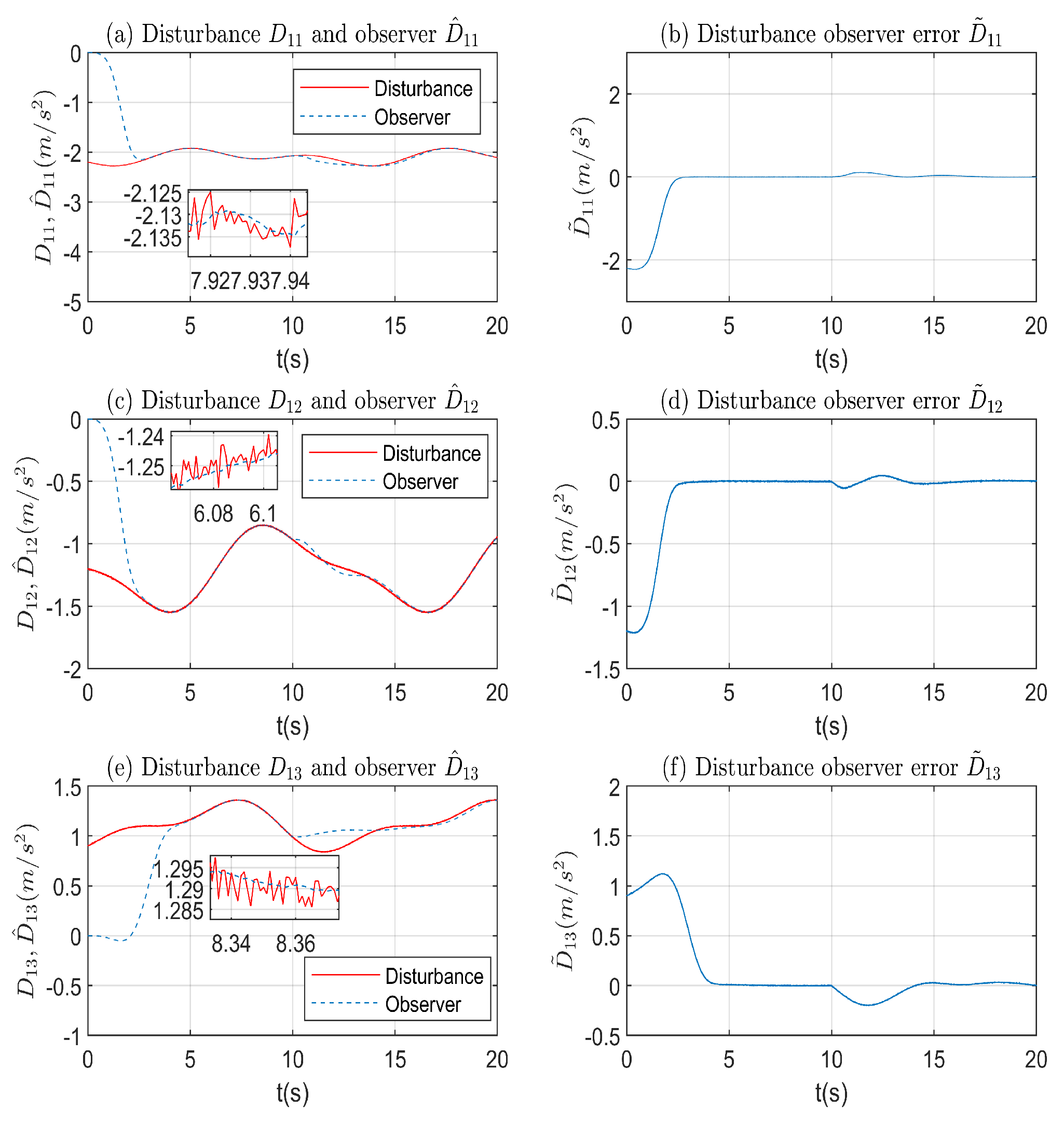
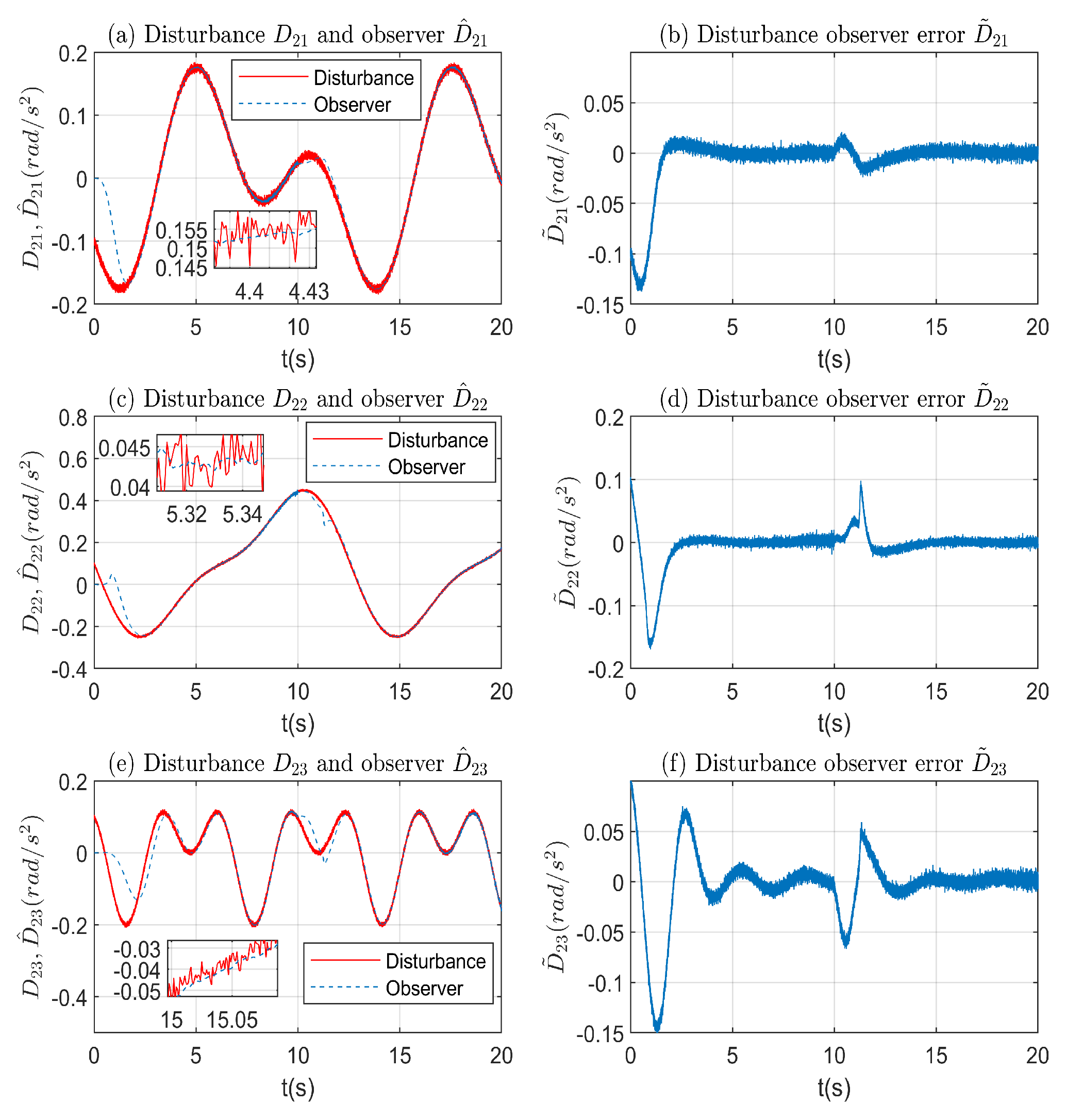
The simulation results in Case 1 are shown in Figure 3, Figure 4, Figure 5 and Figure 6. From Figure 3, it can be seen that, when $0<t\le 10$ s, only the AOA is controlled and, for $10<t\le 20$ s, the total velocity $V_T$, AOA ($\alpha$), and sideslip angle ($\beta$) are all controlled simultaneously. The controlled variables can converge to a small neighborhood around the given values within $4s$ in the presence of uncertainties. The tracking errors of total velocity, AOA, and sideslip angle are $7.5\times {10}^{-4}$ m/s, $6.4\times {10}^{-5}$ deg, and $4.6\times {10}^{-6}$ deg, respectively. Figure 4 illustrates the fluctuation of the control variables in the simulation, including the force control $u_V$, virtual control of angular velocity ${\mathit{W}}_d$, torque vector ${\mathit{u}}_T$, and deflection vector $\mathit{\delta }$ (canard wings ${\delta }_c$, right elevon ${\delta }_{re}$, left elevon ${\delta }_{le}$, and rudder ${\delta }_r$). The control variables can actuate promptly in response to the external disturbances. The actuators are appropriately managed to maintain high tracking performance. Based on Figure 5 and Figure 6, the nonlinear disturbance observers give better estimations of the disturbances. The estimation errors are with the maximum magnitude of ${10}^{-3}$. The simulation results in Case 1 show that the triplet states can be controlled separately and simultaneously in the form of vectors, which illustrate the effectiveness of the developed controller.

4.2. Robustness of the Proposed Nonlinear Disturbance Observer Enhanced Controller

Case 2.

To illustrate the robustness of the proposed nonlinear disturbance observer enhanced controller, the total velocity ($V_T)$, AOA (α) and sideslip angle (β) are controlled under noisy disturbances. The simulation conditions are similar to Case 1, and zero-mean white Gaussian noises are added on the disturbances ${\mathit{D}}_1$ and ${\mathit{D}}_2$ in Equations (60) and (61), respectively. The simulation results in Case 2 are shown from Figure 7, Figure 8, Figure 9 and Figure 10.

Remark 7.

In fact, the lumped disturbances, ${\mathit{D}}_1$ and ${\mathit{D}}_2$, are correlated in a realistic physics environment. However, the correlation is difficult to model and simulate. Then, inspired by the simulations of [4,17,20,27], the uncertainties, ${\mathit{D}}_1$ and ${\mathit{D}}_2$, are selected with white Gaussian noises for illustrating the robustness and filter’s character of the developed nonlinear disturbance observer. Our future research will focus on considering the correlated ${\mathit{D}}_1$ and ${\mathit{D}}_2$ which are state-dependent and develop an adaptive-gain controller under the proposed scheme.

The performance of the developed flight controller against noisy disturbances is evaluated in Case 2. From Figure 7, the reference signals can be quickly tracked even when the noise and the model uncertainties exist simultaneously. The states of the aircraft can be steered to the intended values in a timely manner. The tracking errors of total velocity, AOA, and sideslip angle are $-1.7\times {10}^{-5}$ m/s, $4.4\times {10}^{-5}$ deg, and $7.8\times {10}^{-5}$ deg, respectively. Figure 8 illustrates the fluctuation of the control variables in the simulation. The control variables can actuate promptly in response to the noisy disturbances and the chattering phenomenon exists, but it is not serious in the control inputs. In Figure 9 and Figure 10, the performance of the nonlinear disturbance observers is illustrated. The magnitude of chartering in the observer is much smaller than that in the noise. The disturbance observers can handle noisy disturbances, which can be seen as low-pass filters to some degree, and this reflects the theoretical analysis in Remark 3. In summary, the robustness and applicability of the developed multivariable backstepping sliding mode controller is further verified through the simulation studies in Case 2.

4.3. Comparison with a Decoupled Controller

Case 3.

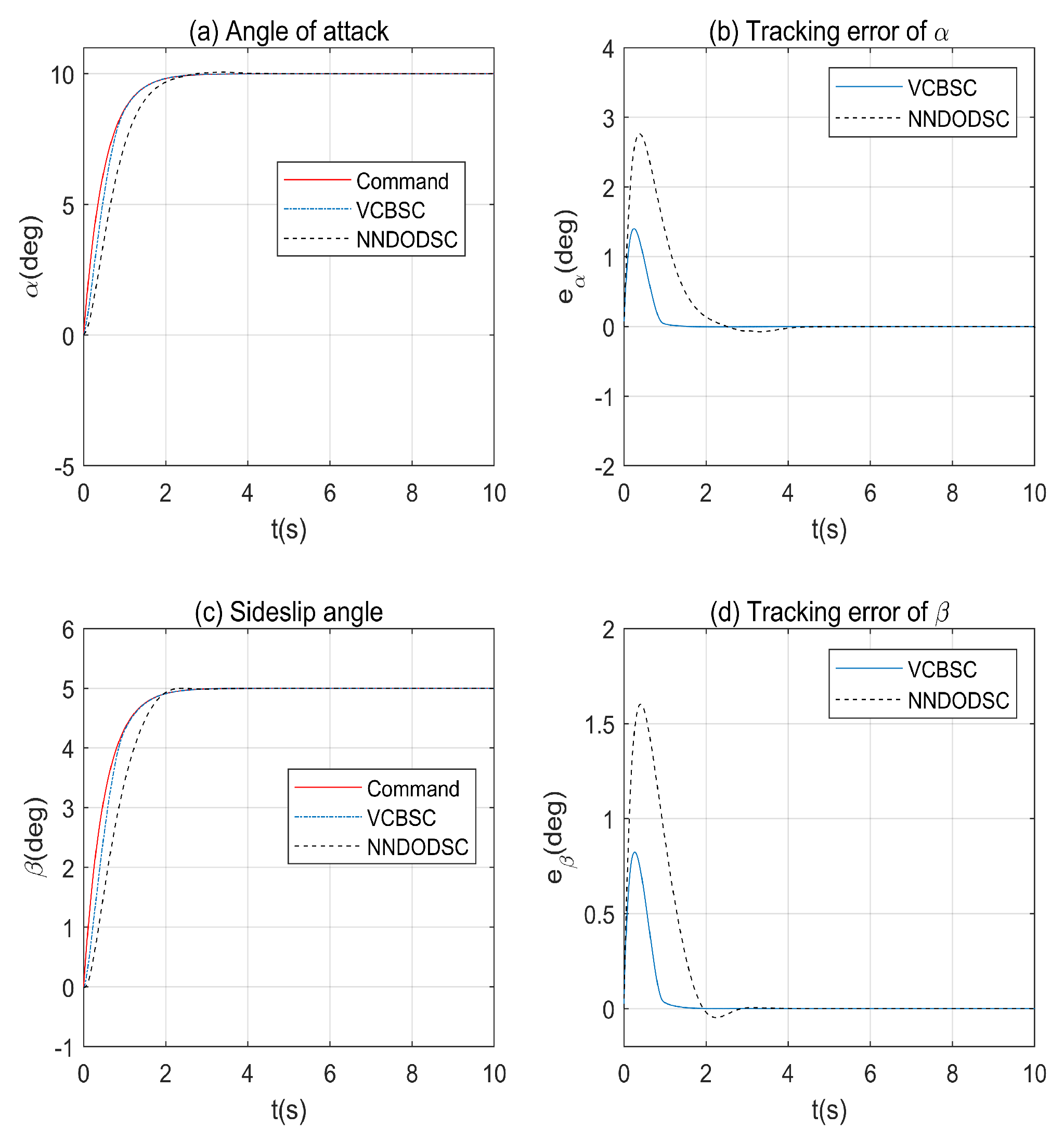
To verify the superiority of the proposed vector-coupled multivariable backstepping sliding mode controller (VCBSC), over our previous work, it is compared with a nonhomogeneous nonlinear disturbance observer-based dynamic surface controller (NNDODSC) presented in [20] through simulations under the same conditions. The NNDODSC is proposed based on the traditional flight control model, which was described as univariate form, i.e., state equations with AOA, sideslip angle, roll angle, roll rate, pitch rate, and yaw rate, and multiple scalar equations were considered and designed using a novel nonhomogeneous nonlinear disturbance observer and dynamic surface control theory. The simulation results in Case 3 are shown in Figure 11 and Figure 12.

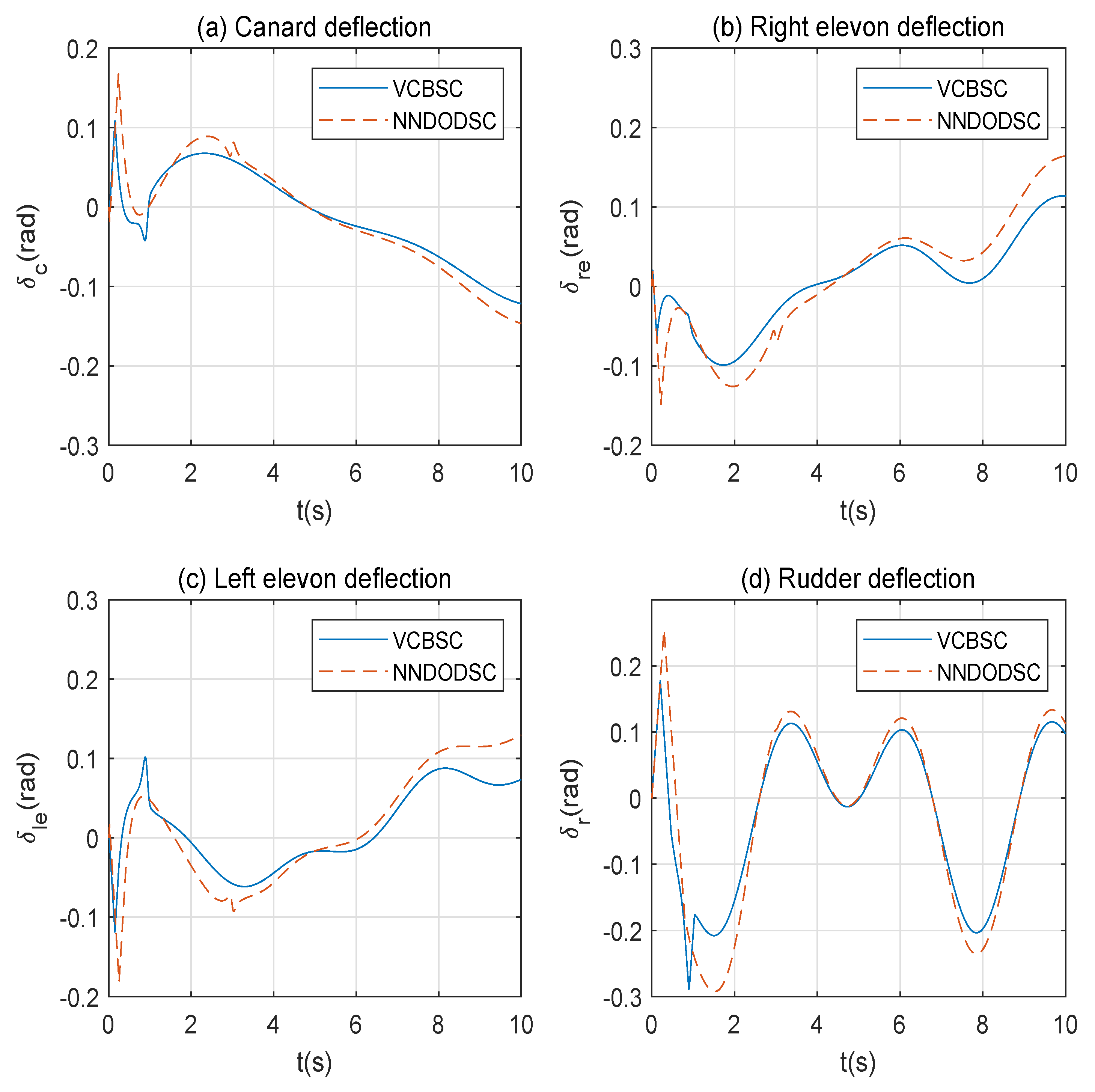
As shown in Figure 11, the AOA and sideslip angle stably follow their respective reference commands, and better tracking performance is achieved with faster convergent rate by using the proposed VCBSC scheme than the traditional decoupled method of the NNDODSC. Moreover, the control inputs of the two control algorithms are shown in Figure 12. In addition, we can detect from Figure 11 and Figure 12, though the control surface deflections under the decoupled controller are larger than those of the proposed vector-coupled controller when $t\in$ [0,4 s], the tracking performance of the decoupled controller is worse and the settling time is longer. Larger control deflections are required for NNDODSC than VCBSC, especially in the initial stage, which illustrates that the proposed combined vector controller, which deals with the inherent cross-coupling in the flight dynamics, can improve the efficiency of the control inputs.

Remark 8.

To testify the superiority of the proposed vector-coupled multivariable backstepping sliding mode controller, we have spent time and effort on regulating the parameters for the decoupled controller by trial and error to make the performance of the closed-loop system as good as possible under the simulation scenario, and make sure that the control surface deflections of the two simulations are nearly the same. Then, it can be guaranteed that the comparison between the two controllers is fair.

Based on the above simulation results, we can conclude that the proposed vectorial controller is effective and robust, the triplet airspeed ($V_T$), AOA ($\alpha$), and sideslip angle ($\beta$) can converge to small regions around the desired commands, and the design objective is achieved: a high control precision can be obtained even in the case of noisy disturbances. This also validates the theoretical analysis results.

5. Conclusions

We developed a vector-coupled control scheme for multivariable flight control based on the Lyapunov stability theory. The controller had a combination of vector sliding mode control, vector backstepping control, and nonlinear distance observers. Our key findings and the main contributions of our investigation are summarized as follows:

• The developed control scheme allowed the conversion of attitude and airspeed control of an aircraft into a space-vector tracking problem. The results showed that the triplet airspeed ($V_T$), AOA ($\alpha$), and sideslip angle ($\beta$) could be controlled separately and simultaneously in the form of vectors. A key feature of this study is the active use of cross-coupling in the flight dynamics instead of decoupling and passive suppression and compensation.
• The use of the Lyapunov stability theory enabled the development of a flight control system that is semi-globally uniformly ultimately bounded. The simulation results were comparable to the theoretical results, and it was shown that the developed controller is effective and robust.
• The developed control scheme is concise and aesthetically more appealing compared with traditional control structures, which uses decoupled collections of single variables. The combined control scheme has a symmetry structure and each term is meaningful. The feature that the control parameters can be considered and adjusted in each term directively is significant.

Our future work will concentrate on adaptive flight control design under the proposed vector-coupled control scheme considering control input saturation.

References

1. Zhu, J.H. A Survey of Advanced Flight Control Theory and Application. In Proceedings of the Conference on Computational Engineering in Systems Applications, Beijing, China, 4–6 October 2007; pp. 655–658. [Google Scholar]
2. Shkolnikov, A.; Shtessel, Y. Aircraft Nonminimum Phase Control in Dynamic Sliding Manifolds. J. Guid. Control Dyn. 2001, 24, 566–571. [Google Scholar] [CrossRef]
3. Zong, Q.; Wang, F.; Tian, B. Nonlinear adaptive filter backstepping flight control for reentry vehicle with input constraint and external disturbances. J. Aerosp. Eng. 2013, 28, 889–907. [Google Scholar] [CrossRef]
4. You, M.; Zong, Q.; Tian, B.; Zhao, X.; Zeng, F. The comprehensive design of uniform robust exact disturbance observer and fixed-time controller for reusable launch vehicles. IET Control Threory Appl. 2018, 12, 638–648. [Google Scholar] [CrossRef]
5. Li, P.; Yu, X.; Zhang, Y. Adaptive Multivariable Integral TSMC of a Hypersonic Gliding Vehicle With Actuator Faults and Model Uncertainties. IEEE/ASME Trans. Mechatron. 2017, 22, 2723–2735. [Google Scholar] [CrossRef]
6. Zhang, L.; Bi, S.; Yang, H. Fuzzy-PID Control Algorithm of the Helicopter Model Flight Attitude Control. In Proceedings of the 2010 Chinese Control and Decision Conference, Xuzhou, China, 26–28 May 2010; pp. 1438–1443. [Google Scholar]
7. Amato, F.; Mattei, M.; Scala, S.; Verde, L. Robust Flight Control Design for the HIRM based on Linear Quadratic Control. Aerosp. Sci. Technol. 2000, 4, 423–438. [Google Scholar] [CrossRef]
8. Yoshimasa, O. Design of a Flight Controller for Hypersonic Flight Experiment Vehicle. Asian J. Control 2004, 6, 353–361. [Google Scholar]
9. Huang, Y.; Xu, K.; Han, J.; Lam, J. Flight Control Design Using Extended State Observer and Non-smooth Feedback. In Proceedings of the 40th IEEE Conference on Decision and Control, Orlando, FL, USA, 4–7 December 2001; pp. 223–228. [Google Scholar]
10. Snell, A.; Enns, D.; Garrard, W. Nonlinear Inversion Flight Control for a Supermaneuverable Aircraft. J. Guid. Control Dyn. 1992, 15, 976–984. [Google Scholar] [CrossRef]
11. Da Costa, R.; Chu, Q.; Mulder, J. Reentry Flight Controller Design Using Nonlinear Dynamic Inversion. J. Guid. Control Dyn. 2003, 40, 64–71. [Google Scholar] [CrossRef]
12. Sonneveldt, L.; Chu, Q.; Mulder, J. Nonlinear Flight Control Design Using Constrained Adaptive Backstepping. J. Guid. Control Dyn. 2007, 30, 322–336. [Google Scholar] [CrossRef]
13. Hao, A.; Fidan, B.; Wu, Q.; Wang, C.; Cao, X. Sliding Mode Differentiator Based Tracking Control of Uncertain Nonlinear Systems with Application to Hypersonic Flight. Asian J. Control 2019, 21, 143–155. [Google Scholar]
14. Castañeda, H.; Salas-Peña, O.; Leon-Morales, J. Robust flight control for a fixed-wing unmanned aerial vehicle using adaptive super-twisting approach. J. Aerosp. Eng. 2014, 228, 2310–2322. [Google Scholar]
15. Nagesh, I.; Edwards, C. A multivariable super-twisting sliding mode approach. Automatica 2014, 50, 984–988. [Google Scholar] [CrossRef] [Green Version]
16. Li, P.; Ma, J.; Zheng, Z. Disturbance-observer-based fixed-time second-order sliding mode control of an air-breathing hypersonic vehicle with actuator faults. J. Aerosp. Eng. 2017, 232, 344–361. [Google Scholar] [CrossRef]
17. Chen, M.; Yu, J. Disturbance Observer-Based Adaptive Sliding Mode Control For Near-Space Vehicles. Nonlinear Dyn. 2015, 15, 1671–1682. [Google Scholar] [CrossRef]
18. Vansoest, W.R.; Chu, Q.P.; Mulder, J.A. Combined feedback linearization and constrained model predictive control for entry flight. J. Guid. Control Dyn. 2006, 29, 427–434. [Google Scholar] [CrossRef]
19. Li, C.Y.; Jing, W.X.; Gao, C.S. Adaptive backstepping-based flight control system using integral filters. Aerosp. Sci. Technol. 2009, 13, 105–113. [Google Scholar] [CrossRef]
20. Ma, J.; Li, P.; Zheng, Z. Disturbance observer based dynamic surface flight control for an uncertain aircraft. J. Aerosp. Eng. 2017, 232, 729–744. [Google Scholar] [CrossRef]
21. Yu, P.; Shtessel, Y. Continuous Higher Order Sliding Mode Control with Adaption of Air Breathing Hypersonic Missile. Int. J. Adapt. Control Signal Process. 2016, 30, 1099–1117. [Google Scholar] [CrossRef]
22. Shtessel, Y. Multiple Time Scale Flight Control Using Re-configurable Sliding Modes. In Proceedings of the AIAA Guidance, Navigation and Control Conference and Exhibit, Hilton Head, SC, USA, 20–23 August 2007; pp. 1–10. [Google Scholar]
23. Dong, Q.; Zong, Q.; Tian, B.; Wang, F. Adaptive-gain multivariable super-twisting sliding mode control for reentry RLV with torque perturbation. Int. J. Robust Nonlinear Control 2016, 27, 620–638. [Google Scholar] [CrossRef]
24. Härkegård, O.; Glad, T. Vector backstepping design for flight control. In Proceedings of the AIAA Guidance, Navigation and Control Conference and Exhibit, Hilton Head, SC, USA, 20–23 August 2007; pp. 1–10. [Google Scholar]
25. Fossena, T.; Berg, S. Nonlinear Vectorial Backstepping Design for Global Exponential Backing of Marine Vessels in the Presence of Actuator Dynamics. In Proceedings of the 36th Conference on Decision and Control, San Diego, CA, USA, 12 December 2003; pp. 4237–4242. [Google Scholar]
26. Bates, D.; Hagström, M. Nonlinear Analysis and Synthesis Techniques for Aircraft Control; Springer: Berlin, Geramany, 2007. [Google Scholar]
27. Tian, B.; Yin, L.; Wang, H. Finite Time Reentry Attitude Control Based on Adaptive Multivariable Disturbance Compensation. IEEE Trans. Ind. Electron. 2015, 62, 5889–5898. [Google Scholar] [CrossRef]
28. Yu, X.; Li, P.; Zhang, Y. The design of fixed-time observer and finite-time fault-tolerant control for hypersonic gliding vehicles. IEEE Trans. Ind. Electron. 2017, 65, 4135–4144. [Google Scholar] [CrossRef]
29. Lie, F.; Pradipta, A.; Gebre-Egziabher, D. Synthetic Air Data System. J. Aircr. 2013, 50, 1234–1249. [Google Scholar] [CrossRef]
30. Chen, W. Disturbance observer based control for nonlinear systems. IEEE/ASME Trans. Mechatron. 2004, 9, 706–710. [Google Scholar] [CrossRef]
31. Swaroop, D. Dynamic Surface Control of Nonlinear Systems. In Proceedings of the American Control Conference Albuquerque, Albuquerque, NM, USA, 6 June 1997; pp. 3028–3034. [Google Scholar]
32. Swaroop, D. Dynamic Surface Control for Nonlinear Systems. IEEE Trans. Autom. Control 2000, 45, 1893–1899. [Google Scholar] [CrossRef]
33. Forssell, L.; Nilsson, U. ADMIRE the Aero-Data Model in a Research Environment Version 4.0, Model Description; Technical Report, FOI-R-1624-SE; FOI: Stockholm, Sweden, 2005. [Google Scholar]
Figure 1. Flight model with inertial frame Σ i , body-fixed frame Σ b , and wind frame Σ w .
Symmetry 11 01225 g001
Figure 2. Schematic of the control structure.
Symmetry 11 01225 g002
Figure 3. Case 1: flight states: (a) airspeed V T ; (c) angle of attack α ; (e) angle of sideslip β ; and their tracking errors: (b) tracking error of V T ; (d) tracking error of α ; (f) tracking error of β .
Symmetry 11 01225 g003
Figure 4. Case 1: control variables: (a) force control u V ; (b) virtual angular velocity W d ; (c) angular acceleration control u T ; and deflection vector δ : (d) canard wings δ c ; (e) right elevon δ r e ; (f) left elevon δ l e , and (g) rudder δ r .
Symmetry 11 01225 g004
Figure 5. Case 1: (a) the disturbance D 11 and its observer D ^ 11 ; (b) the estimation error D ˜ 11 ; (c) the disturbance D 12 and its observer D ^ 12 ; (d) the estimation error D ˜ 12 ; (e) the disturbance D 13 and its observer D ^ 13 ; (f) the estimation error D ˜ 13 .
Symmetry 11 01225 g005
Figure 6. Case 1: (a) the disturbance D 21 and its observer D ^ 21 ; (b) the estimation error D ˜ 21 ; (c) the disturbance D 22 and its observer D ^ 22 ; (d) the estimation error D ˜ 22 ; (e) the disturbance D 23 and its observer D ^ 23 ; (f) the estimation error D ˜ 23 .
Symmetry 11 01225 g006
Figure 7. Case 2: flight states: (a) airspeed V T ; (c) angle of attack α ; (e) angle of sideslip β ; and their tracking errors: (b) tracking error of V T ; (d) tracking error of α ; (f) tracking error of β .
Symmetry 11 01225 g007
Figure 8. Case 2: control variables: (a) force control u V ; (b) virtual angular velocity W d ; (c) angular acceleration control u T ; and deflection vector δ : (d) canard wings δ c ; (e) right elevon δ r e ; (f) left elevon δ l e , and (g) rudder δ r .
Symmetry 11 01225 g008
Figure 9. Case 2: (a) the disturbance D 11 and its observer D ^ 11 ; (b) the estimation error D ˜ 11 ; (c) the disturbance D 12 and its observer D ^ 12 ; (d) the estimation error D ˜ 12 ; (e) the disturbance D 13 and its observer D ^ 13 ; (f) the estimation error D ˜ 13 .
Symmetry 11 01225 g009
Figure 10. Case 2: (a) the disturbance D 21 and its observer D ^ 21 ; (b) the estimation error D ˜ 21 ; (c) the disturbance D 22 and its observer D ^ 22 ; (d) the estimation error D ˜ 22 ; (e) the disturbance D 23 and its observer D ^ 23 ; (f) the estimation error D ˜ 23 .
Symmetry 11 01225 g010
Figure 11. Case 3: flight states: (a) angle of attack α ; (c) angle of sideslip β ; and their tracking errors: (b) tracking error of α ; (d) tracking error of β .
Symmetry 11 01225 g011
Figure 12. Case 3: (a) canard wings δ c ; (b) right elevon δ r e ; (c) left elevon δ l e ; and (d) rudder δ r .
Symmetry 11 01225 g012