Article

Software Tool for Acausal Physical Modelling and Simulation

1
Department of Computer Science and Numerical Analysis, University of Cordoba, Campus Rabanales, 14071 Cordoba, Spain
2
Department of Mechanical Engineering, University of Cordoba, Campus Rabanales, 14071 Cordoba, Spain
*
Author to whom correspondence should be addressed.
Symmetry 2019, 11(10), 1199; https://doi.org/10.3390/sym11101199
Submission received: 8 August 2019 / Revised: 13 September 2019 / Accepted: 17 September 2019 / Published: 24 September 2019

Abstract

:
Modelling and simulation are key tools for analysis and design of systems and processes from almost any scientific or engineering discipline. Models of complex systems are typically built on acausal Differential-Algebraic Equations (DAE) and discrete events using Object-Oriented Modelling (OOM) languages, and some of their key concepts can be explained as symmetries. To obtain a computer executable version from the original model, several algorithms, based on bipartite symmetric graphs, must be applied for automatic equation generation, removing alias equations, computational causality assignment, equation sorting, discrete-event processing or index reduction. In this paper, an open source tool according to OOM paradigm and developed in MATLAB is introduced. It implements such algorithms adding an educational perspective about how they work, since the step by step results obtained after processing the model equations can be shown. The tool also allows to create models using its own OOM language and to simulate the final executable equation set. It was used by students in a modelling and simulation course of the Automatic Control and Industrial Electronics Engineering degree, showing a significant improvement in their understanding and learning of the abovementioned topics after their assessment.

Graphical Abstract

1. Introduction

First-principles modelling of complex systems with continuous and discrete components (hybrid systems), which arises in many different fields, is a challenging task that can be efficiently carried out using the Object-Oriented Modelling (OOM) paradigm [1,2]. OOM allows to handle this complexity by structuring the overall model in a modular and hierarchical way using smaller basic components organized in libraries that can be reused [3]. Models created with OOM languages have a declarative nature [4], i.e., they are acausal (without preassigned computational causality in the model equations) in contrast to procedural or block-oriented modelling languages. This feature allows one to focus on creating the model without worrying about obtaining a computer executable equation set ready for simulation because this task (called partition generation) is automatically carried out by algorithms implemented in OOM tools [5,6]. Currently, Modelica [7] is considered a de facto standard of OOM languages and is used in most of both commercial and open source OOM tools (Dymola [8], SimulationX [9], OpenModelica [10], MapleSim [11], etc.), though there are other tools not based on Modelica, such as gPROMS [12] or EcosimPro [13,14]. Key features common to all OOM languages are [3]:
• Encapsulation: isolation of a component internal mathematical description and associated data from its external interface, allowing the modeller to deal with model complexity in an easier way. Encapsulation is typically implemented through the class concept. It is a pattern which defines both the component private part (dynamic equations, discrete events, local variables and internal topology) and its public part (parameters, attributes and connection ports). An object or component is an instantiation of a class, and an abstract (or partial) class only describes the common or generic behaviour and data that will be inherited by different components. All objects instantiated from a class are constrained to the same structure data and behaviour defined on it, so this concept of class can be explained as symmetry [15].
• Inheritance: mechanism that allows common behaviours and interfaces to be shared between components. It simplifies the modelling task and makes possible the creation of class libraries (packages) organized in a hierarchical way with interrelated parent and derived classes (the latter can be considered a specialization of the former). Depending on the number of parent classes used, inheritance can be simple (only one parent class) or multiple (several parent classes). The specialization concept with invariant data and behaviour between a subclass and its parent classes is also related to symmetry [15].
• Aggregation: creation of components from others previously developed and debugged (objects of more basic classes), so that they can be reused. This mechanism can be iteratively applied with no limit, so a final component can be extremely complex if it is built through aggregation of many other simpler ones.
A lot of models that have been created using the OOM paradigm can be found on the literature. To cite just a few recent works from several fields, there are examples of mechanical systems [16,17,18], electrical systems [19,20,21], thermal systems [22,23,24,25], energy systems [26,27,28,29] and processes [30,31]. This clearly shows that OOM is a very useful methodology for modelling multidisciplinary complex systems.
On the other hand, it has been proven that software tools used as teaching support of certain subjects allow a better understanding of its key concepts by the students. In general, the introduction of these tools has led, to some extent, to an improvement in their learning. For example, in automatic control, graphical and interactive tools created in different environments, such as MATLAB [32,33,34], Sysquake [35,36] or Easy Java/Javascript Simulation [37], represent a suitable and easy way of explaining and illustrating non-intuitive contents that are difficult to understand. Reviewing recent state of the art, many other different topics in which educational tools have been introduced can be found, including electronics [38], physics [39,40], mechanical engineering [41,42], thermodynamics [43], optics [44] or robotics [45]. In all these works, developed tools proved to be powerful and valuable instruments for improving student learning.
This work introduces a software tool focused on system modelling and simulation according to the OOM paradigm with added educational capabilities. The tool has been developed for creating and simulating models as well as for learning an OOM language and understanding how the algorithms for partition generation work. These last two topics have been the main motivation to create the tool; firstly, the OOM language implemented on it is a subset of Modelica, including its main features, so it is easier to learn for novice users (in this case, students with no previous knowledge about the OOM paradigm); secondly, the tool can show partial results from partition generation algorithms (via ordered equations and incidence matrices), so that the user can observe all equation processing steps from model source code, which is of great interest for students attending a modelling and simulation course. Hence, the tool implements all the OOM paradigm’s key features and shows graphically, step by step, the process of obtaining the final equation set for simulation. Such features are not found in other solutions mainly focused on obtaining, as quickly as possible, the final equation set for simulation (making the process transparent to the user) and not on educational aspects. As previously stated, OOM is widely used in many fields, so the developed tool can be a useful complement for engineering students to learn effectively this methodology.
The paper is organized as follows: concepts about DAE systems, their relationship with OOM and the algorithms frequently used for partition generation are explained in Section 2. Description of the key tool features and the use of its Graphical User Interface (GUI) is carried out in Section 3. Section 4 provides several didactic examples included with the tool and explains the partition generation and simulation results obtained from that cases. Student evaluation and assessment after using the tool is described in Section 5. Finally, conclusions are summarized in Section 6.

2. Background

2.1. Differential-Algebraic Equation Systems

Dynamical models of complex physical systems are often built using differential equations with algebraic restrictions [1,6], thus constituting a Differential-Algebraic Equation (DAE) system [46]. The general form of these systems is:
f x , x , z , t = 0
g x , z , t = 0
where x’ are the derivatives of state variables x, z are the algebraic variables and t is the time. Equation (1) represents the differential (dynamical) part of the system and Equation (2) is the set of algebraic restrictions [47]. Previous equation systems frequently arise if the OOM paradigm is used to create a model which, as stated before, is one of the most efficient alternatives when the system to be modelled is complex. Post-processing of these equations through several steps, i.e., partition generation, is necessary to obtain a final executable equation set [5,6]. Algorithms applied to this task are mainly based on bipartite symmetric graphs.

2.2. Partition Generation

After obtaining the initial equation set from the model source code, in the first step, the model variables must be classified into constant, parameter, algebraic, state or derivative ones. Constants never change their values, and parameters can do it between simulations (although not during execution of a simulation). Initial conditions of the state variables are assumed known. The category of each variable is explicitly defined on the model source code or obtained using symbolic processing.
In the second step, alias equations (i.e., equations whose structure is a = b) are removed [5], reducing the size of the system. Only one of the variables involved in alias equations is preserved for each deleted alias equation.
Computational causality assignment is the third step. It determines which unknown is computed from which equation [5,48]. For this purpose, the original incidence matrix is built, whose rows represent the model equations, and its columns represent the unknowns (derivative and algebraic variables). The matrix element (i,j) is “1” if unknown j is involved in equation i, and is “0” otherwise, so this matrix is mostly sparse [49]. Then, a Dulmage-Mendelsohn permutation [50] is applied to the original incidence matrix. This algorithm sorts the incidence matrix into blocks, and assigns computational causality to the equations [51,52]. The resulting incidence matrix is typically lower triangular, whose main diagonal contains “1s”; all the elements above the main diagonal are “0s”, and the order of its rows and columns is modified with respect to the original incidence matrix. Each element of the main diagonal determines which unknown is computed from which equation.

2.3. Algebraic Loops

Previous algorithms have difficulties with systems like the one shown in (3,4). Unknown x needs to be computed before unknown y (3), but this is not possible without having previously calculated unknown x (4). Therefore, no variable can be computed without knowing the other one. In this case, the system presents an algebraic loop, which often appears with connected model components [5].
y = f x
x = g y
When the Dulmage-Mendelsohn permutation is applied to systems like (3,4), a sorted block lower triangular incidence matrix is obtained (with some elements “1” above the main diagonal). This indicates that unknowns in each block must be jointly resolved and, hence, the equation system is isolated using symbolic processing.
Algebraic loops can be linear or non-linear, depending on the type of equations involved in the loop, and they are resolved in a different way [53,54]. When all equations are linear with respect to its unknowns in a block of the sorted incidence matrix, you have a linear algebraic loop. In this case, both well-known symbolic and numerical solvers can be used in the subsequent code generation stage. If the block is non-linear, the Newton-Raphson method can be used iterating the non-linear Equations (5) and (6) after having computed the Jacobian function until the absolute and relative errors are lower than an upper bound.
F z = 0
z n + 1 = z n J 1 z n · F z n
where z are the non-linear unknowns, J is the Jacobian of F(z) with respect to z and n is the iteration number. To prevent the expensive computing of the inverse Jacobian (J-1), the system (7) on unknowns zn+1 can be solved as an alternative.
J z n · z n z n + 1 = F z n

2.4. Higher Index DAEs

The index of a DAE is defined as the number of times the equation system (1,2) must be derived with respect to time t to determine (x’, z’) as a continuous function of x, z and t [47,55]. For example, an index-0 system is a set of ODE (Ordinary Differential Equations) and index 1 means that there is an algebraic loop. Numerical algorithms used to solve DAE [56] will fail if its index is greater than 1 [57]; such DAE has a structural singularity and is called higher index or overdetermined system [1]. In practice, this means that two or more state variables are not mutually independent, that is, some of them are not true state variables. This situation can arise when some components of complex systems are connected using an OOM language [5]. When the Dulmage–Mendelsohn permutation is applied to a higher index system, some rows of the sorted incidence matrix only contain “0s” (no unknown is solved from these equations, which are called singular equations).
An index reduction method must be used to solve this problem, like the Pantelides’ algorithm [57,58,59], which can be applied in most cases. It states that singular equations must be derived with respect to time and, for each one, a state variable must become algebraic [60], which means it will not be integrated. These derivatives of singular equations are added to the initial system because the number of unknowns increases. Each step of Pantelides’ algorithm reduces the system index by one, so it must be iteratively applied until index 1 is obtained (algebraic loop). Depending on the system, it can be more computationally advantageous, relaxing some state variables instead of others.

2.5. Events

Mathematical models of physical systems can reproduce their behaviour up to a certain degree of accuracy. Fast dynamics complicate the simulation and, typically, do not improve precision, so that these dynamics are incorporated in the so-called hybrid systems [2] by adding some discrete equations. Discrete equations are executed when a boolean condition, called event, is triggered. The purpose of these equations is to take the system to a new state after the processed event, where it can be simulated by the DAE solver yet again.
In an OOM language, the discrete equations are enclosed into programming structures which define the set of conditions which triggers an event. During integration of the system, when the conditions associated to an event become true, integration stops and discrete equations are “activated” [2]. Evaluation of these equations is instantaneous, that is, they do not add any lag to simulation time. After execution of the discrete equations, continuous integration is resumed by the solver using the resulting values of state variables as its new initial conditions. To determine the exact time instant in which the event is triggered, all the conditions are converted into crossing functions, monitored by the solver during continuous integration. If any of them crosses zero, the solver computes the exact instant of the crossing, it stops integration and then executes the discrete equations.

3. Developed Tool

Object-Oriented Modeling tool from University of Cordoba (OOMUCO) is a software tool developed in MATLAB 2018a [61] aiming to create and simulate models according to the OOM paradigm and to help students to learn an OOM language and understand how partition and simulation algorithms work. It is an open source project, available at http://www.uco.es/grupos/prinia/wp-content/uploads/OOMUCO.zip, which comprises a simple editor, a compiler and a simulator. Figure 1 shows the relationship between these software components and the workflow from model creation to simulation. Figure 1a shows the editor component, which allows the user to visualize and edit the model source code; the compiler component, which makes parsing of the model source code and translates it into MATLAB code and the simulator component, which carries out the model simulation and shows graphically its results. To describe models, OOMUCO uses a subset of Modelica specification [62] as OOM language.
The user has two complementary alternatives for programming the model of a system in OOMUCO. The first one is to directly write the model equations, specifying variables, parameters, constants, states, etc. The second one is to use library components and link them through connections using specific language sentences. Both options can be combined when the user writes the model in the text editor. The compiler checks source code’s syntax and then applies the algorithms described in Section 2 to obtain an executable equation set in MATLAB code. OOMUCO handles the equations in a symbolic way, i.e., it allows exact differentiation of equations and symbolic resolution of equation systems.
The simulation process is shown in Figure 1b. The compiler checks the model source code, and if it contains no errors, the user can run the simulator, specifying the parameters’ values, state variables’ initial values and simulation time. Thus, several simulations can be carried out with one single compilation. The simulator uses a 4th or 5th order Runge-Kutta integration method, and its simulation results can be viewed graphically (plots of variables selected by the user) or its data saved into a file.

3.1. Object-Oriented Modelling Features in OOMUCO

As previously stated, OOMUCO uses a subset of Modelica OOM specification so that it implements typical features such as classes, types, connections (ports), specialized classes, partial models (abstract classes) and inheritance [62].
To define connectors, OOMUCO uses the specialized class connector, which specifies the variables to interchange between connected objects. For example, the first step to write a library of electronic components is to define the class which connects them, as it is shown in Source code 1.
Source code 1. Connector class “Pin”
connector Pin
 Real v “pin voltage”;
 flow Real I “pin current”;
end Pin;
In this case, variables v of connected Pins will have the same value and the sum of their currents i will be equal to zero (as indicated by the reserved word flow). Therefore, connector classes allow defining how the information between connected components is interchanged. For example, two instances of class Pin (named Pin1 and Pin2) can be declared into two other classes (components) and connect them using the sentence connect(Pin1, Pin2), which generates the equations Pin1.v = Pin2.v and Pin1.i + Pin2.i = 0.
A model can be partially defined, that is, it is not intended to be instantiated, but it can be used to describe a generic (abstract) common behaviour through its variables and equations, which will be inherited by some sub-models. For example, a generic object including two connectors components’ common behaviour can be created (Source code 2) and then it can be reused to describe specific circuit elements, such as a resistor.
Source code 2. Partial model of a two-connector component
partial model TwoPins
 Pin p, n;
 Real v, I;
equations
 i = p.i;
 v = p.v - n.v;
 p.i + n.i = 0;
end Pin;
Inheritance can be expressed through the reserved word extends. The child class inherits the equations and variables of the parent. As an example, how inheritance is used for Resistor component, which inherits from TwoPins, is shown in Source code 3.
Source code 3. Component Resistor, an example of inheritance
partial model Resistor extends TwoPins
parameter Real R = 1e3 “Units Ohm”;
equations
 v = R * i;
end Resistor;
The specialized class package is used to define libraries of components, structured in a hierarchical way, which can be instantiated or reused. Reserved word import can be used to import a library into ant component’s source code. OOMUCO provides both electrical, electronic and mechanical libraries with basic components so that the students can use them in their models and analyse how they are built.

3.2. Graphical User Interface

OOMUCO’s GUI allows the user to create, edit, compile and simulate models created with its own OOM language. It contains menu entries to access all application’s functionality.
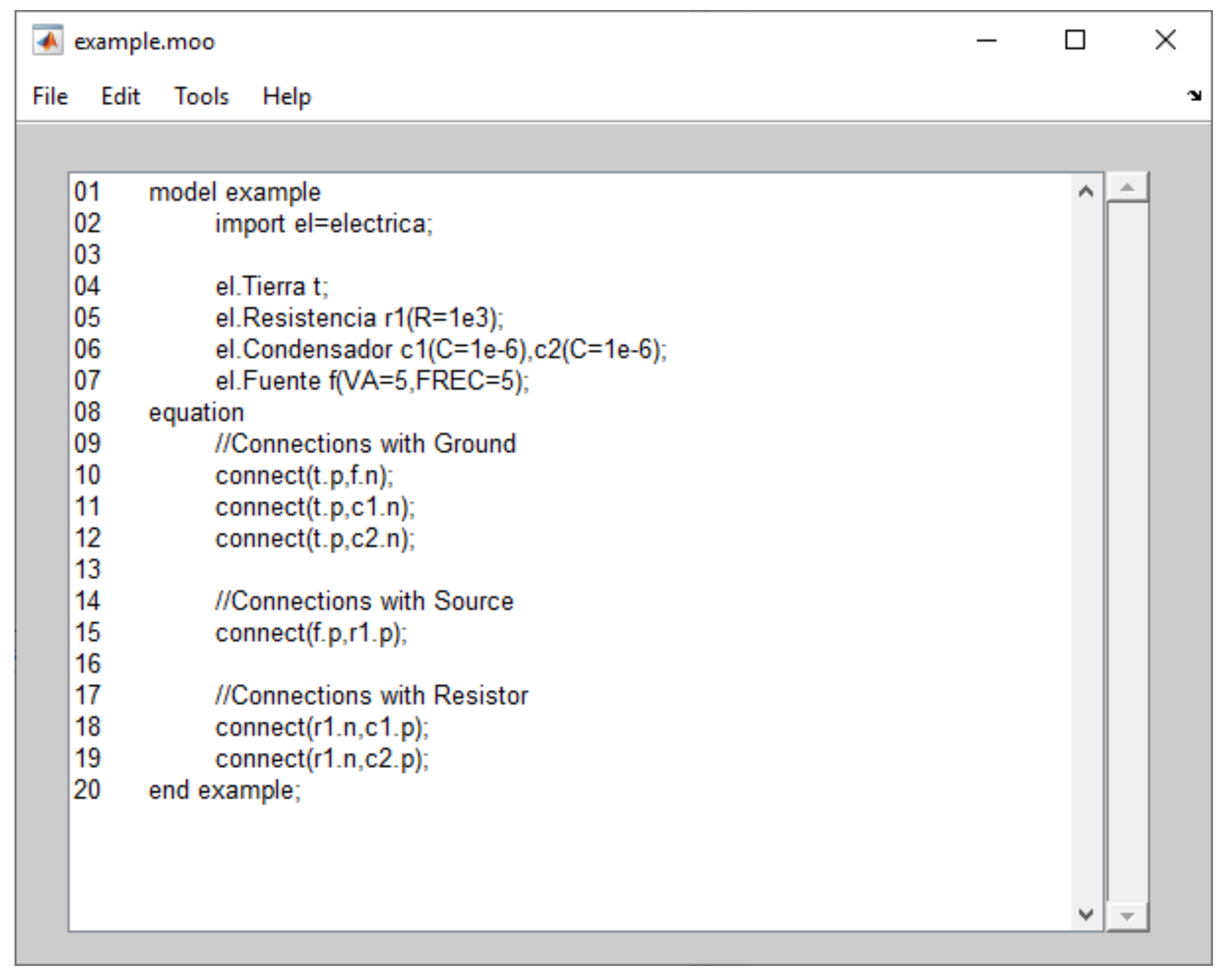
The “Load File…” menu item of the “File” menu loads a model source code file. They are plain text files with .moo extension. If the model is successfully loaded, its source code is shown in the main window (Figure 2). On the other hand, the “Exit” menu item of the “File” menu quits the application.
If a model has been loaded, the user can edit its source code with “Edit with Notepad” menu item of the “Edit” menu. All saved changes will be displayed in OOMUCO’s main window.
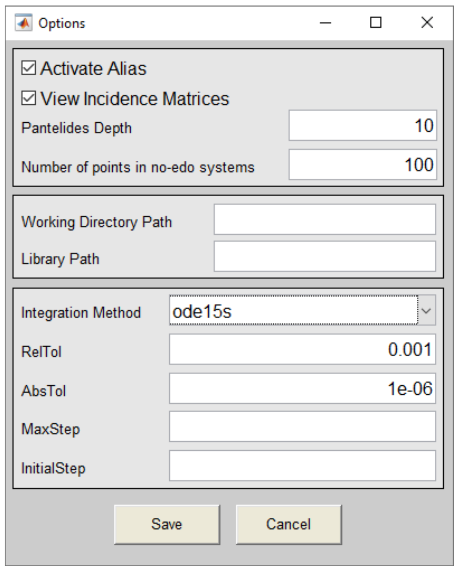
The “Options…” menu item of “Tools” menu (Figure 3) shows the options dialog box. It mainly configures OOMUCO’s behaviour when generating partition and simulating the loaded model.
The “Activate Alias” option turns the alias removal algorithms on or off and the active “View Incidence Matrices” option allows successively viewing, step by step, each of the incidence matrices which are obtained when Dulmage-Mendelsohn permutation, Pantelides’ algorithm and/or algebraic loops processing are applied. The Working Directory and Library paths configure the tool’s root directory and libraries directory, respectively. Finally, some options for the Runge-Kutta integration method (integration algorithm for stiffness, relative tolerance, absolute tolerance, etc.) are also set in the dialog box.
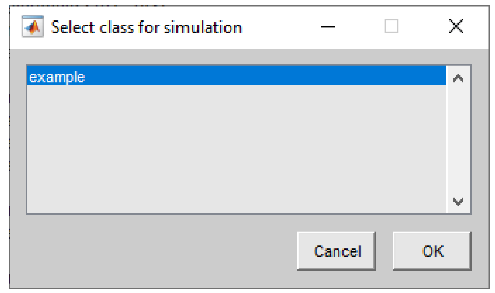
The “Compile…” menu entry of the “Tools” menu launch the partition generation process. At first, the user must choose the component (class) to be processed (Figure 4).
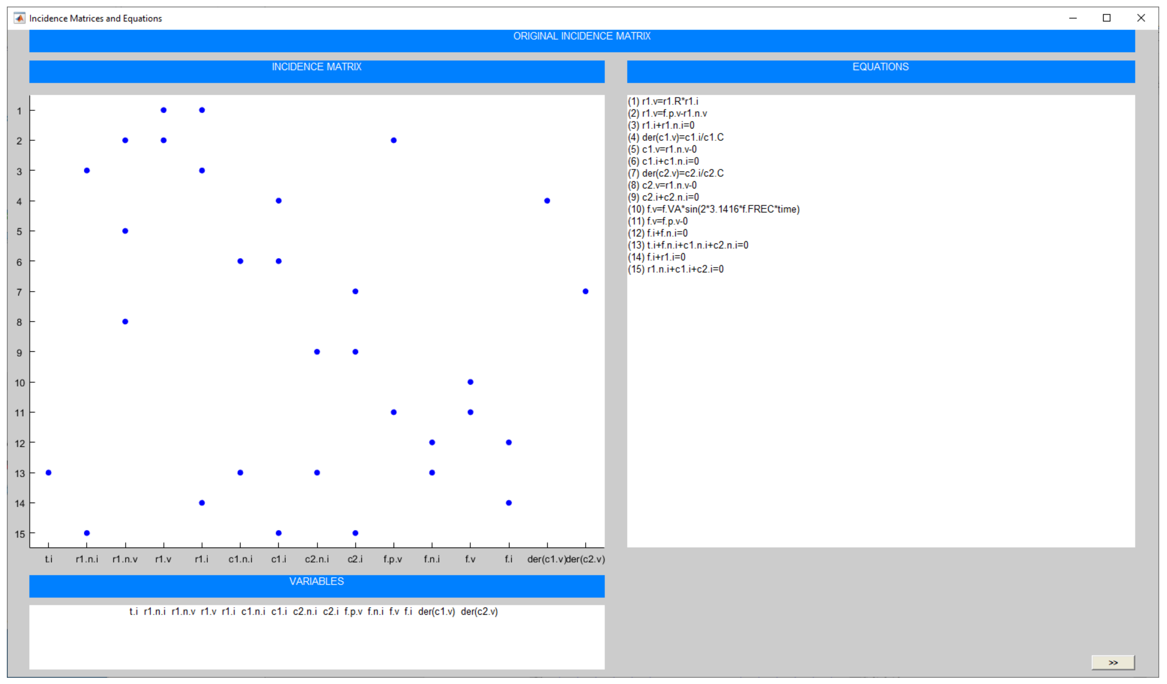
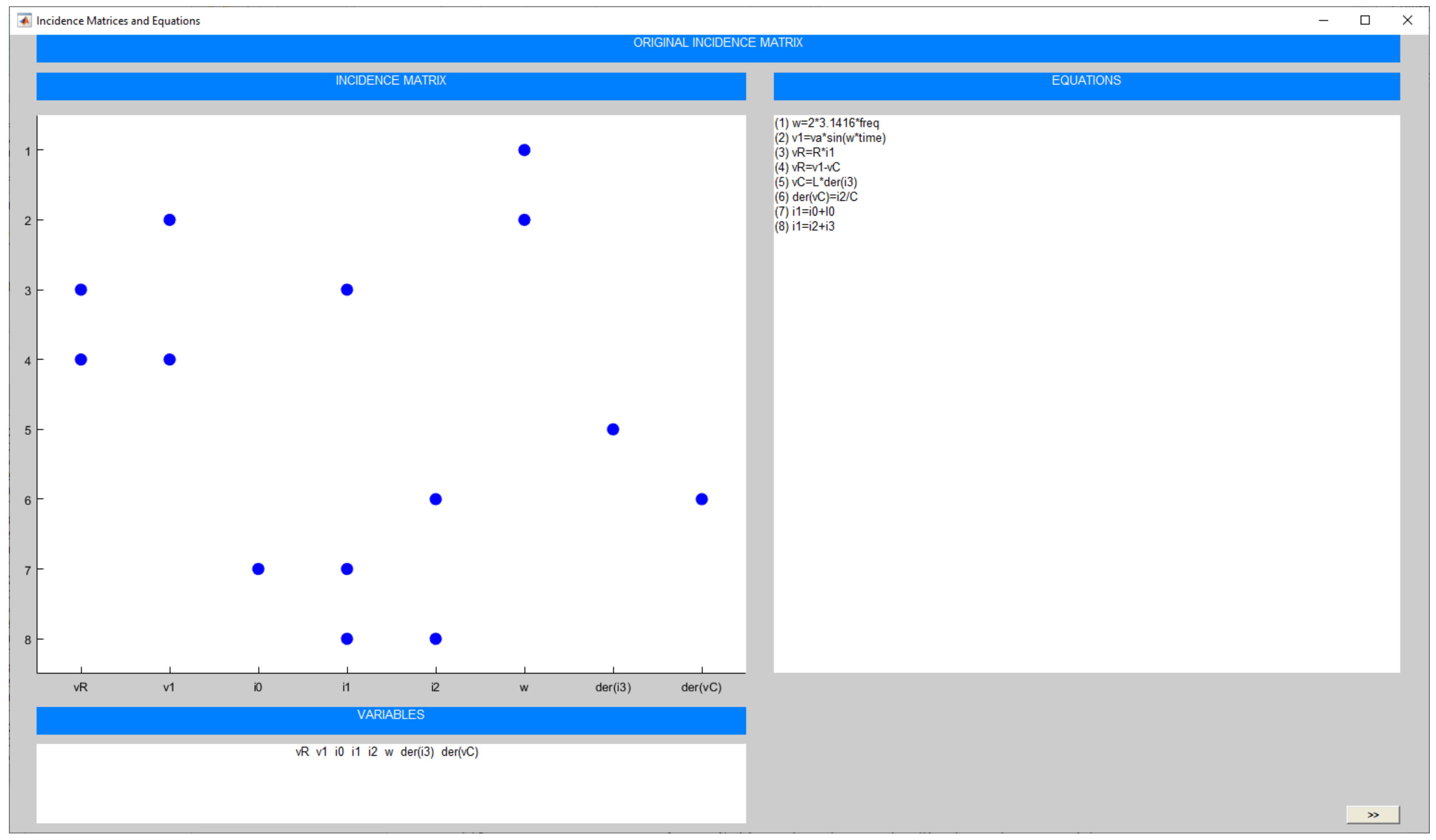
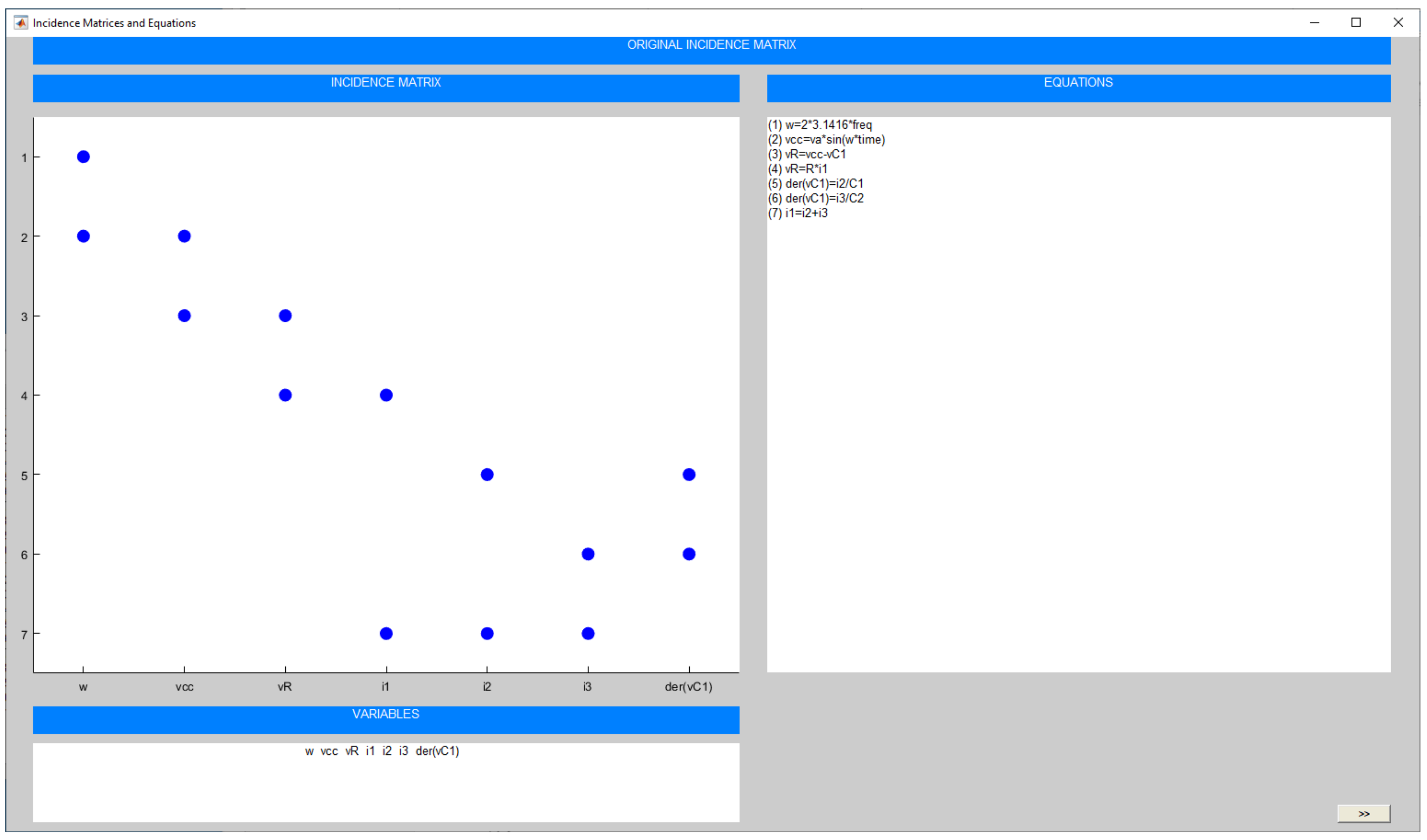
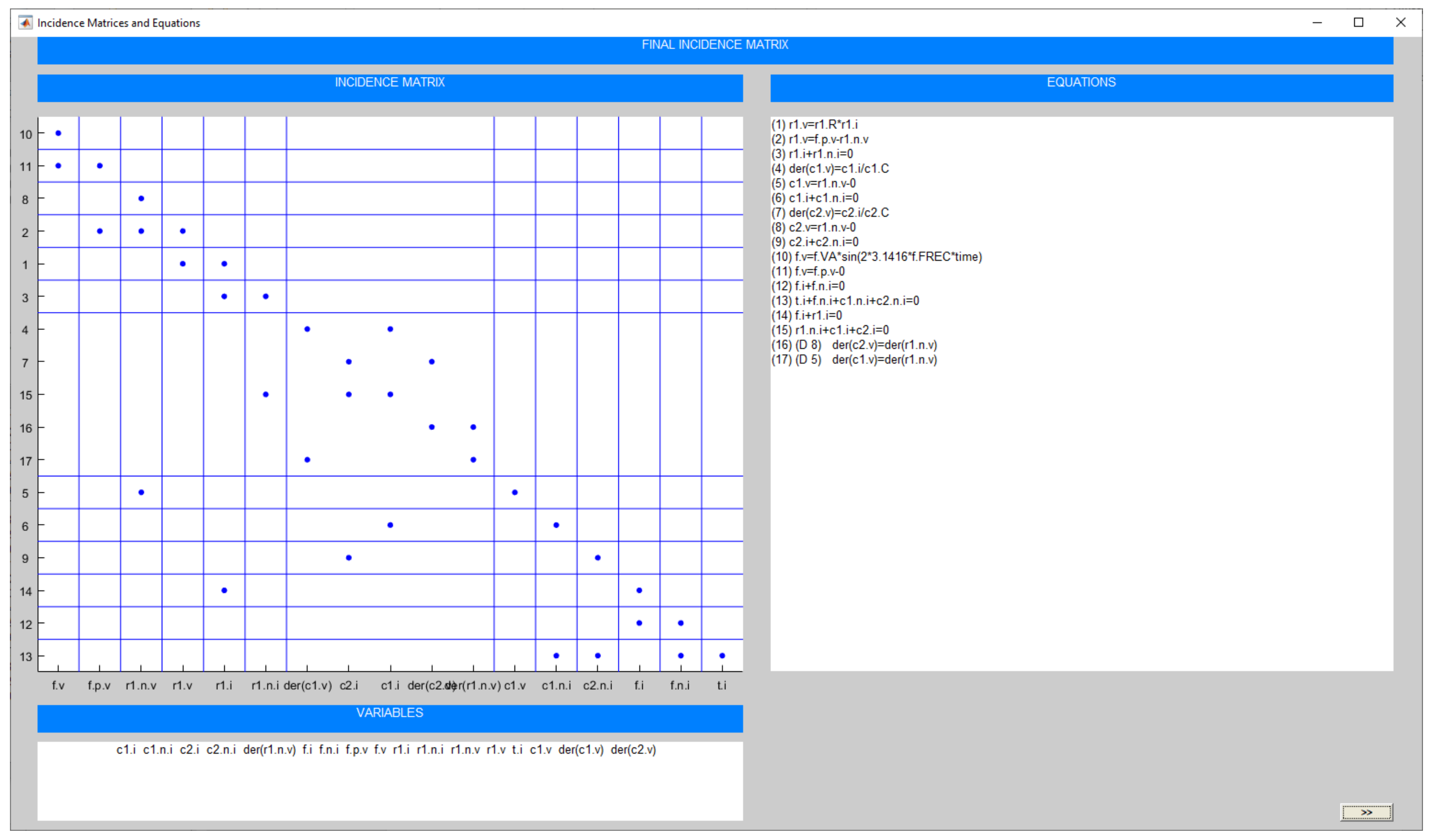
If “View Incidence Matrices” option is off, partition generation process is transparently carried out, except in cases where user intervention is required. If this option is on, then the original incidence matrix and equations are shown (Figure 5). With the “>>” button, the user can observe the results obtained after each algorithm’s processing through the successive sorted incidence matrices and equations. The user can watch, step by step, unknowns-equations pairings and which unknowns, equations and/or state variables are removed by alias removal algorithm or involved in algebraic loops or structural singularities. Depending on the problems found, several user actions can be requested or not. After processing, the final incidence matrix and sorted equations are shown (Figure 6).
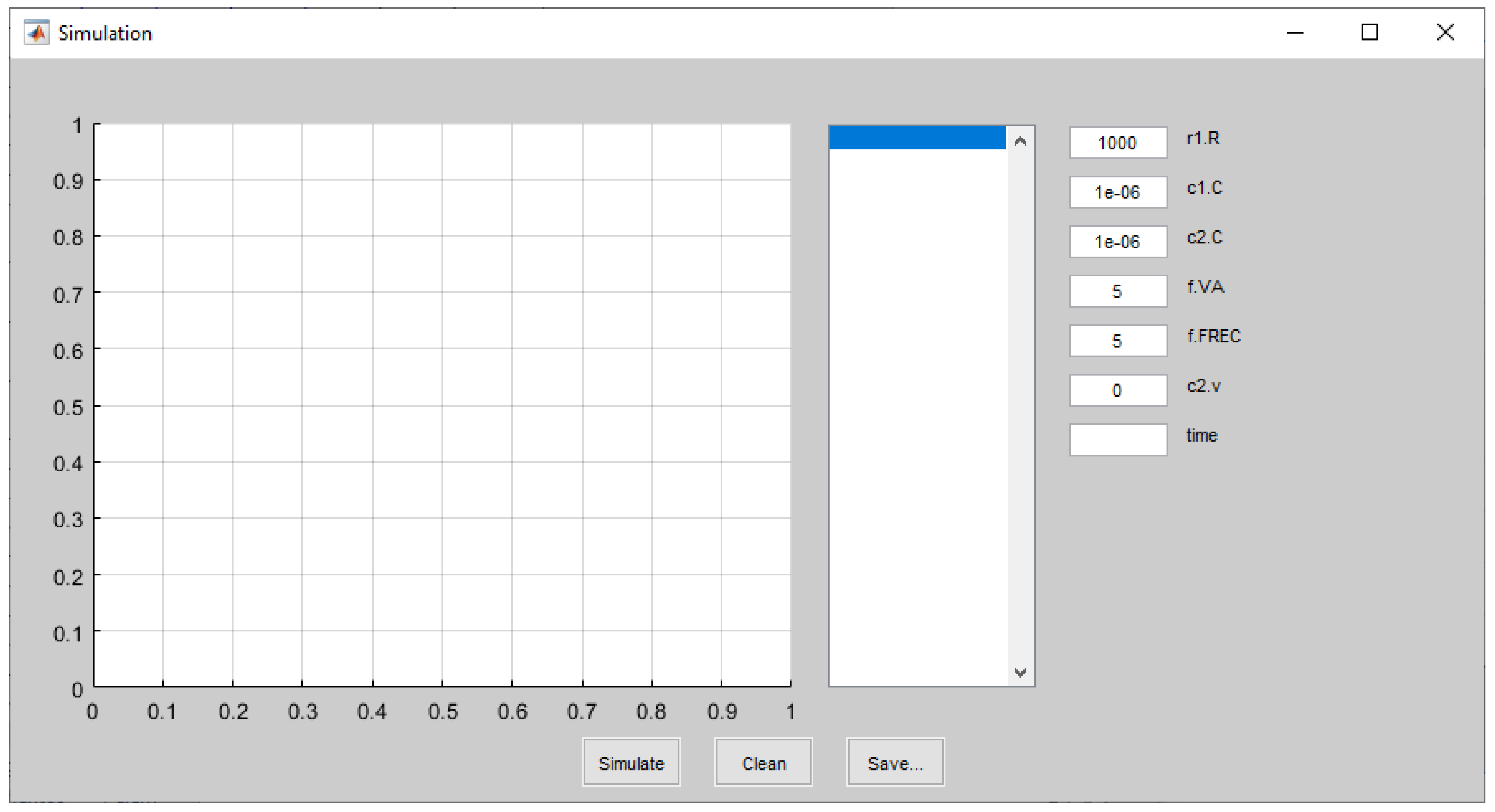
After partition generation, the model can be simulated. The “Simulate…” menu entry of “Tools” menu will be enabled if a partition has been generated and will display a graphical window (Figure 7). The user can modify values of the model’s parameters and constants and must specify the state variables’ initial values and simulation time.
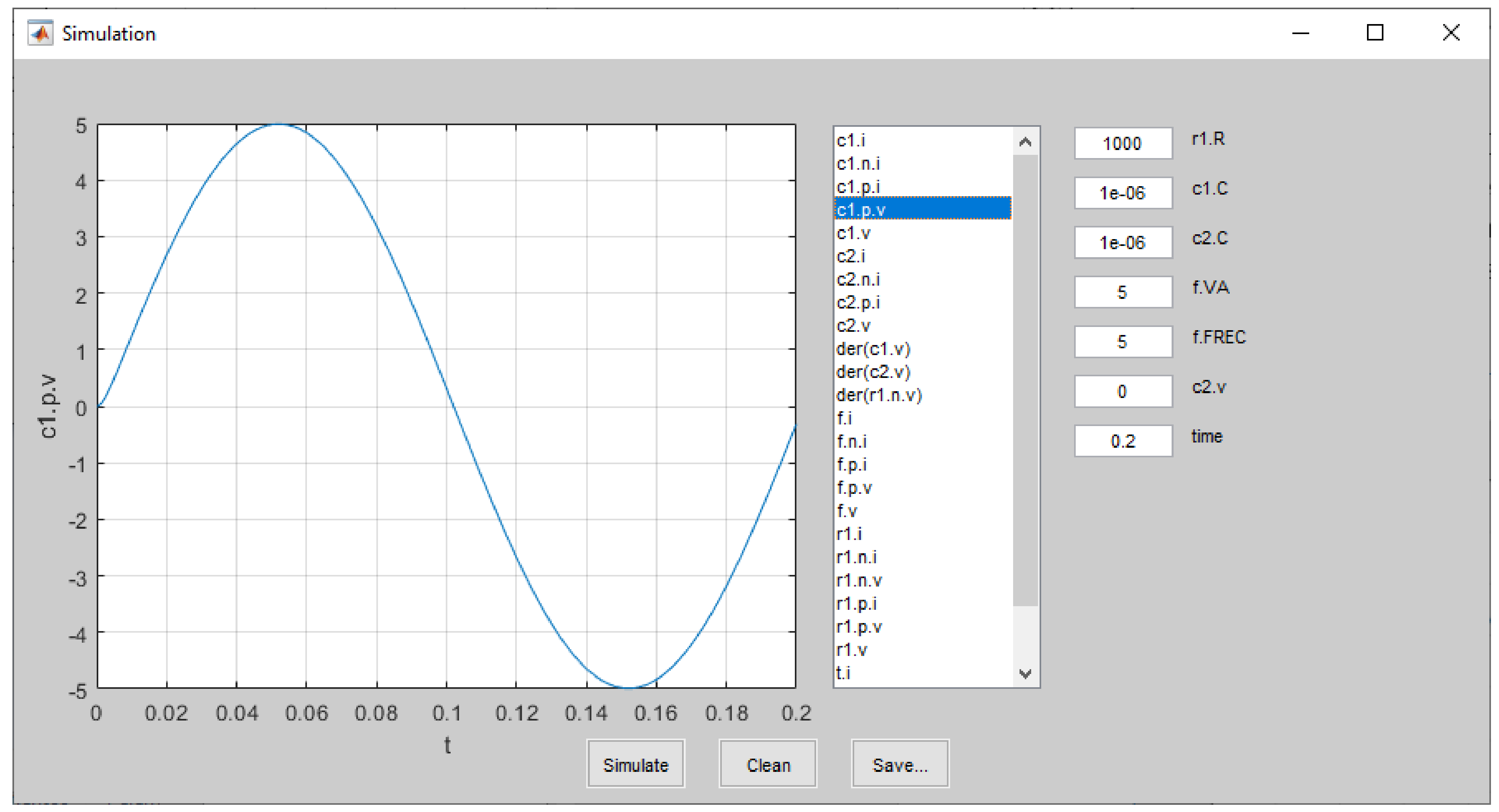
Then, the user must click on the “Simulate” button. All the model’s unknows and state variables will be displayed on the center list, and the user can select several of them to be graphically displayed using the same axes (Figure 8) or saved on to disk (using the “Save…” button). The “Clean” button will only erase all graphics, not the simulation data.

4. Examples

OOMUCO provides several representative instructional examples suitable for teaching students the use of an OOM language and how partition generation algorithms work. These examples cover alias removal, algebraic loops (linear and non-linear), higher index systems, events processing, etc. Some of them will be shown in the next subsections.

4.1. Index-0 DAE System

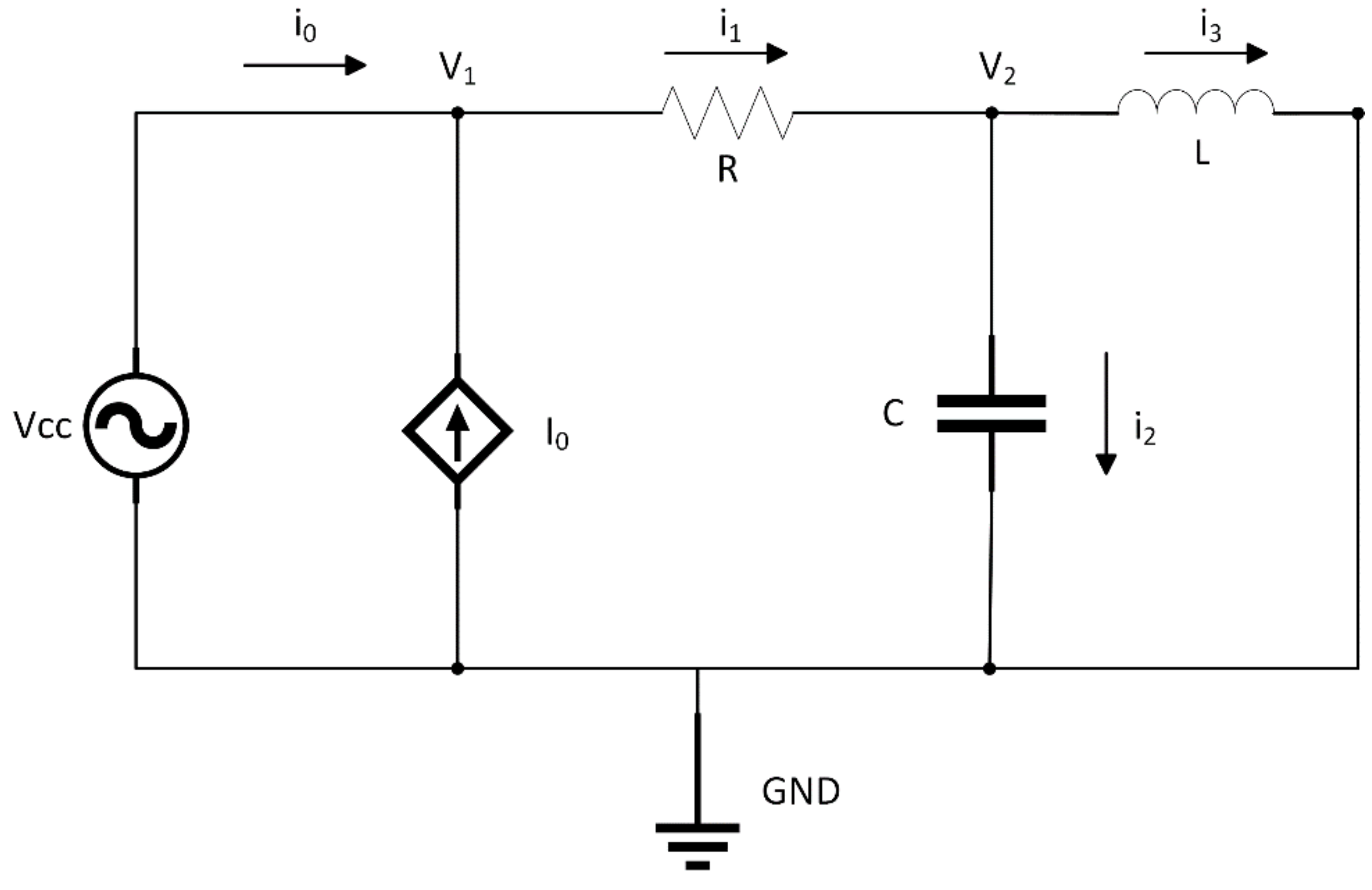
Partition generation and simulation of an index-0 DAE system will be carried out in this example, a simple electrical circuit shown in Figure 9. Applying Kirchhoff’s laws, the DAE system representing its dynamics is (8−18).
V c c = A · sin 2 · P I · F r e q · T I M E
V c c = V 1
V R = R · i 1
V R = V 1 V 2
V L = L · d i 3 d t
V L = V 2
d V C d t = i 2 C
V C = V 2
V 1 = V 0
i 1 = i 0 + I 0
i 1 = i 2 + i 3
where A is the amplitude of the input voltage Vcc.
The differential part of the DAE is modelled by equations (12) and (14) and the algebraic part is composed of the remaining equations. These equations cannot be simulated in any environment in this form. However, this can be done in an OOM environment like OOMUCO. The source code of this model is shown in Source code 4.
Source code 4. Model of electrical circuit (index-0 DAE example)
model circuit
 // Declarations of model constants and parameters
constant Real PI = 3.1415926;
parameter Real A = 5;
parameter Real Freq = 50;
parameter Real C = 4.7e-6;
parameter Real L = 1e-3;
parameter Real R = 1e3;
parameter Real I0 = 0.05;
 // Declarations of model variables
 Real vcc, vR, vL, vC(start=0), v0, v1, v2;
 Real i0, i1, i2, i3(start=0);
equations
 // Equations from Kirchhoff’s laws
 v1 = A*sin(2*PI*Freq*TIME);
 v1 = vcc;
 vR = R*i1;
 vR = v1-v2;
 vL = L*der(i3); “Dynamic equation”
 vL = v2;
 der(vC) = i2/C; “Dynamic equation”
 vC = v2;
 v1 = v0;
 i1 = i0+I0;
 i1 = i2+i3;
end circuit;
In the first step, variables are classified as constants (PI), parameters (VA, Freq, C, L, R, I0), state variables (vC, i3), derivatives (der(vC), der(i3)) and algebraic variables (i0, i1, i2, v0, v1, v2, vR, vL, vcc). In the second step, alias equations ((9), (13), (15) and (16)) are removed by the compiler, thus reducing the size of the system. Note that Equations (9) and (16) link variables v1, vcc and v0, and Equations (8) and (10) link variables vL, v2 and vC. The compiler selects one variable from each of these groups and replaces the remaining ones with them in the equations. Thus, the equation system at this stage is (19−25).
V c c = A · sin 2 · P I · F r e q · T I M E
V R = R · i 1
V R = V c c V C
V C = L · d i 3 d t
d V C d t = i 2 C
i 1 = i 0 + I 0
i 1 = i 2 + i 3
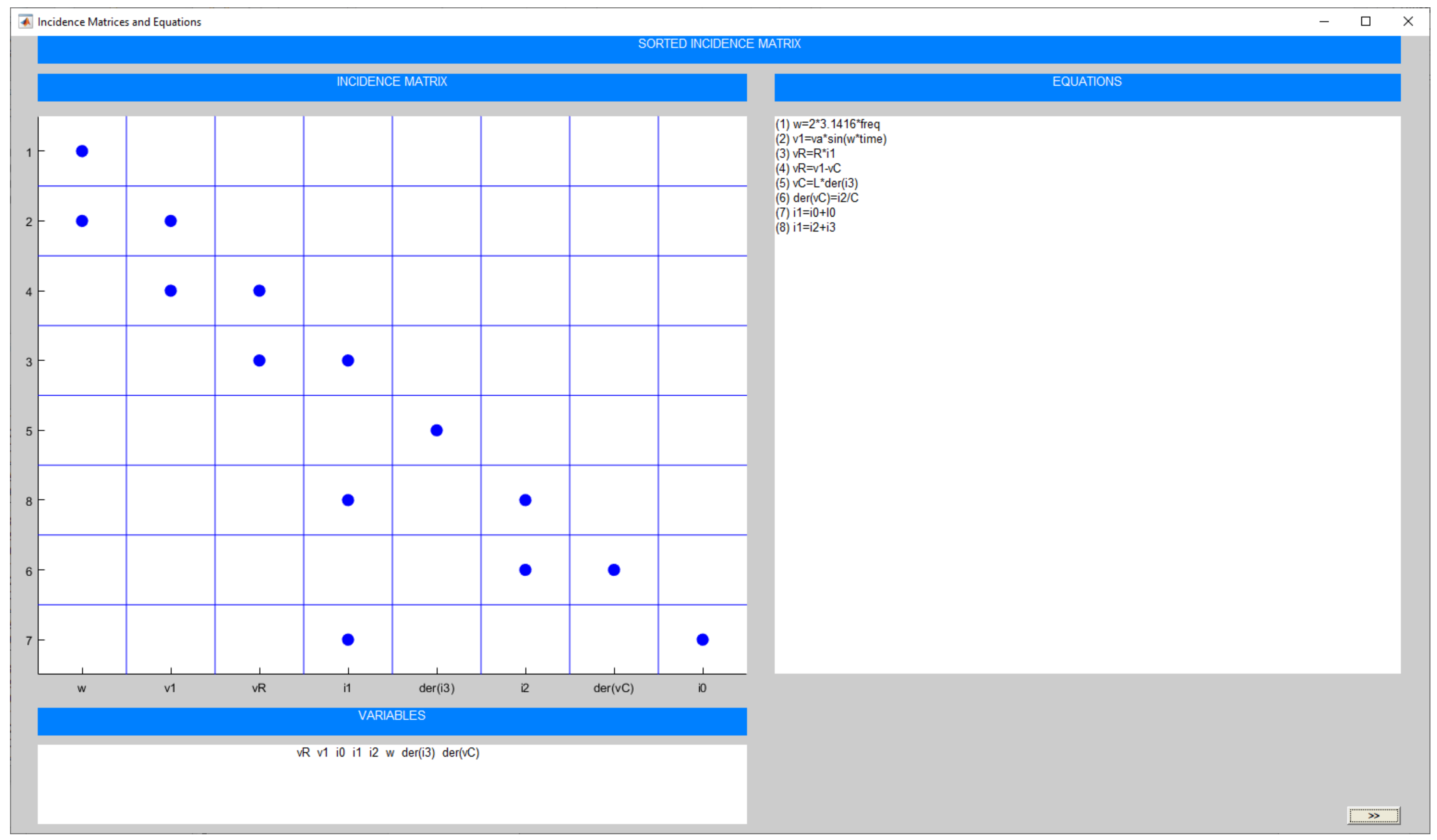
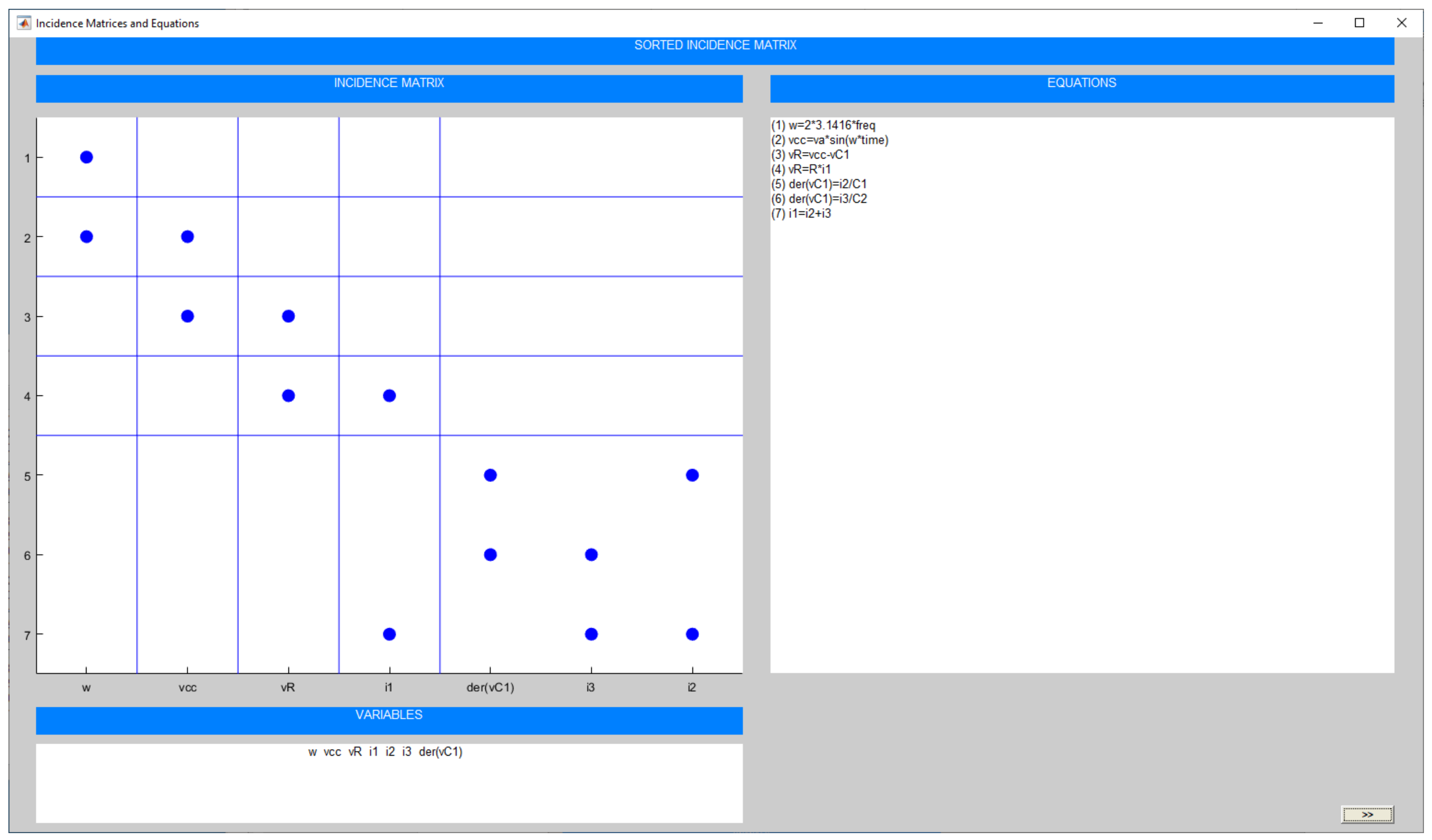
In the third step, automatic assignment of computational causality is carried out by the compiler using symbolic processing. To do this, the original incidence matrix is built as explained in Section 2.2 (Figure 10) and the Dulmage-Mendelsohn permutation is applied to it. The result is a sorted scalar lower triangular incidence matrix (Figure 11), which implies the system is an index-0 DAE. Model simulation is shown in Figure 12.
As can be seen in Figure 12, variables v1, der(vC) and der(i3) were selected for plotting with a simulation time of 0.02 s. Neither model parameter values nor states variables’ initial values were altered. Notice the plot of variable v1, which shows that it is a senoid with a frequency of 50 Hz, equal to vcc, as stated by Equation (9).

4.2. Algebraic Loop

Consider the DAE system (26−28).
d x d t = x + z
3 z 6 y = 9
4 z + 2 y = x
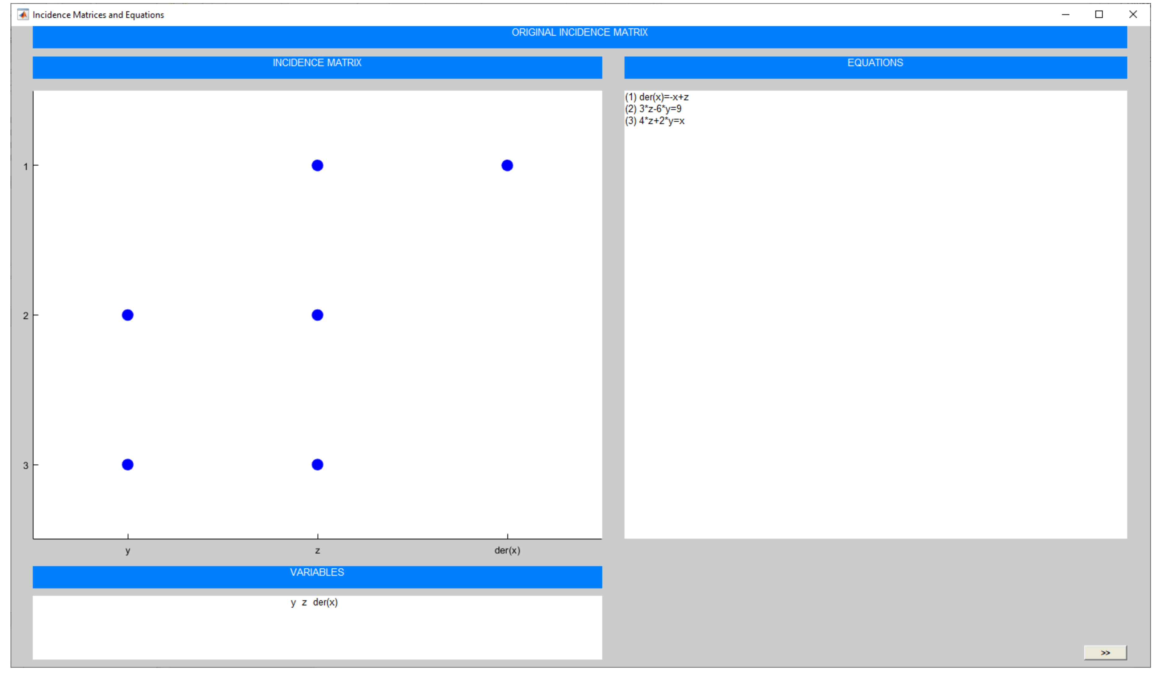
The original and sorted incidence matrices are shown in Figure 13 and Figure 14, respectively.
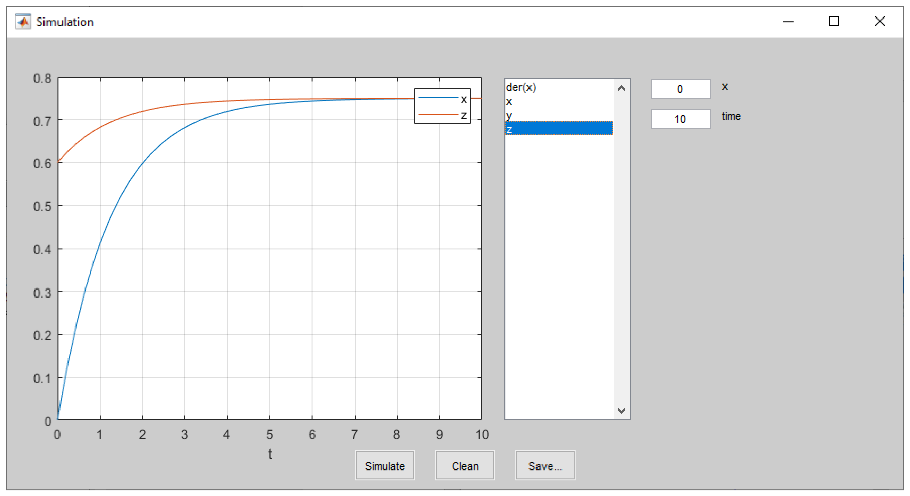
The sorted incidence matrix is block lower triangular with two diagonal blocks. The first one is 2 × 2 and constituted by Equations (27) and (28) with unknowns y-z. The second block is 1 × 1 and constituted by Equation (26) with unknown x ˙ . In the syntax analysis stage, the compiler detects that the first block corresponds to a linear algebraic loop, which is isolated and symbollicaly processed for faster simulation execution. Equations (29)–(31) and Figure 15 show the obtained system and simulation results, respectively.
z = x + 3 5
y = x + 12 10
d x d t = x + z
At stationary state, z = x from Equation (31), so variables x and z reach the same stationary value of 3/4 = 0.75 from Equation (29), as it is shown in Figure 15. On the other hand, initial value of variable z is 3/5 = 0.6 because x = 0 at zero time.

4.3. Higher Index System

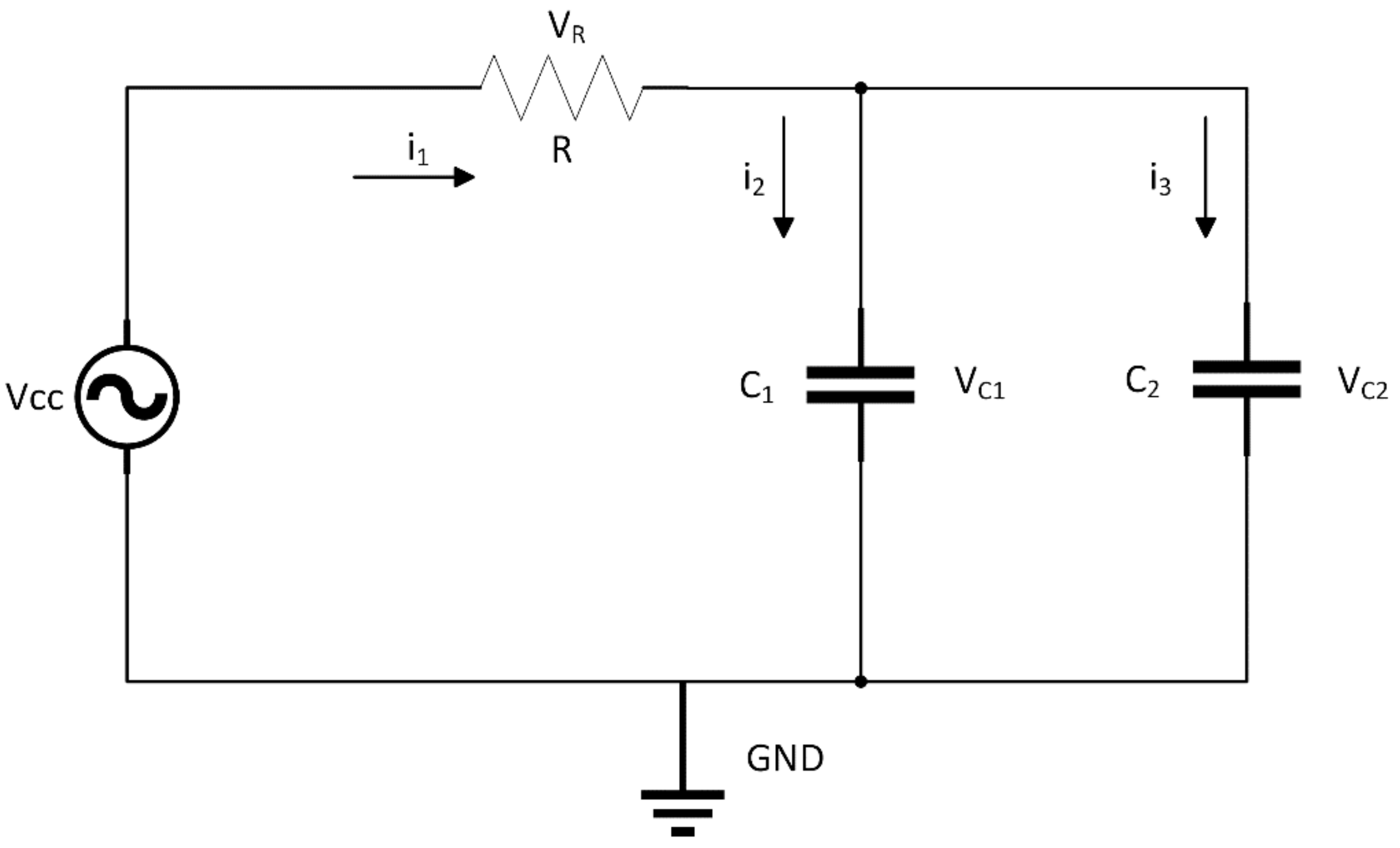
A classical example of higher index system is an electrical circuit with two capacitors in parallel (Figure 16). Directly applying Kirchhoff’s laws directly, Equations (32)−(38) can be obtained.
V c c = A · s i n w · t
V R = V c c V C 1
V R = R · i 1
d V C 1 d t = i 2 C 1
d V C 2 d t = i 3 C 2
V C 1 = V C 2
i 1 = i 2 + i 3
From Equations (35) and (36), initially there are two state variables, the voltage of the two capacitors VC1 and VC2, but from Equation (37) (singular equation), it is clear that both are equivalent, and therefore, they are not independent. Thus, DAE (32−38) is an overdetermined system.
As stated in 2.2, alias equations are removed as one of the first steps of the partition generation. Equation (37) is clearly an alias equation, so it is removed from the system, and only VC1 or VC2 is preserved. In fact, when OOMUCO compiles the model, VC2 does not even appear in the initial incidence matrix (Figure 17) since it has been substituted by VC1 in all equations. Hence, in this case, index reduction has been carried out through alias removal, and the sorted incidence matrix (Figure 18) only shows an algebraic loop.
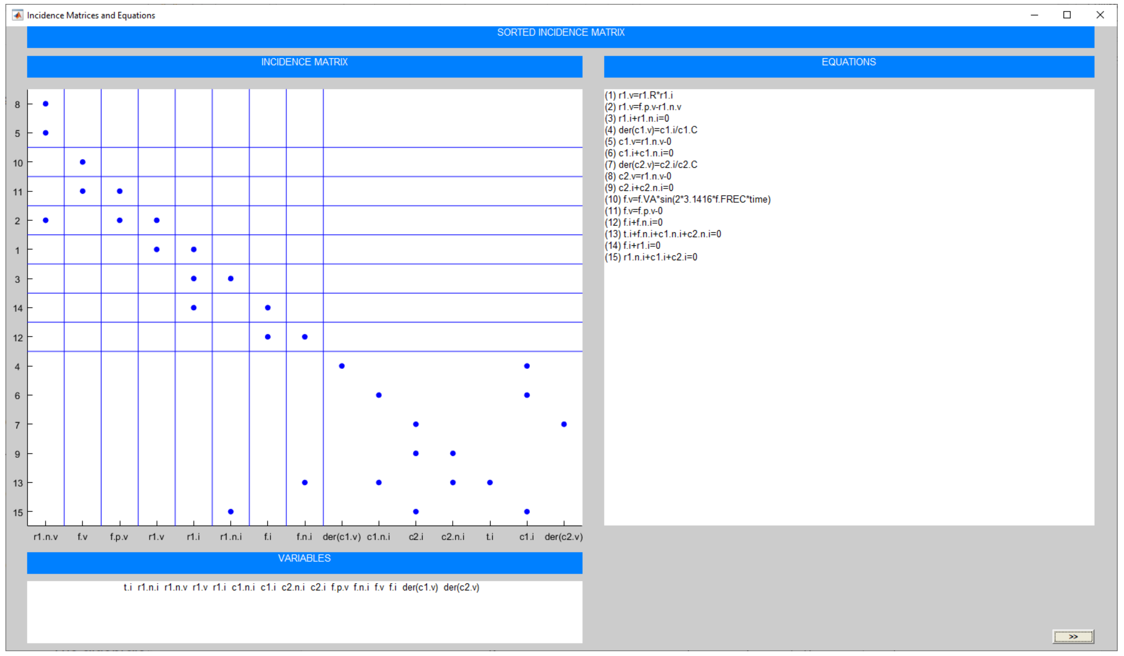
This system can also be modelled by means of the OOM paradigm, as it is shown in Figure 2 using the “electrica” library provided by OOMUCO. The first sorted incidence matrix (Figure 19) shows that no unknown is solved from equation 5 (singular equation), confirming that it is a higher index system.
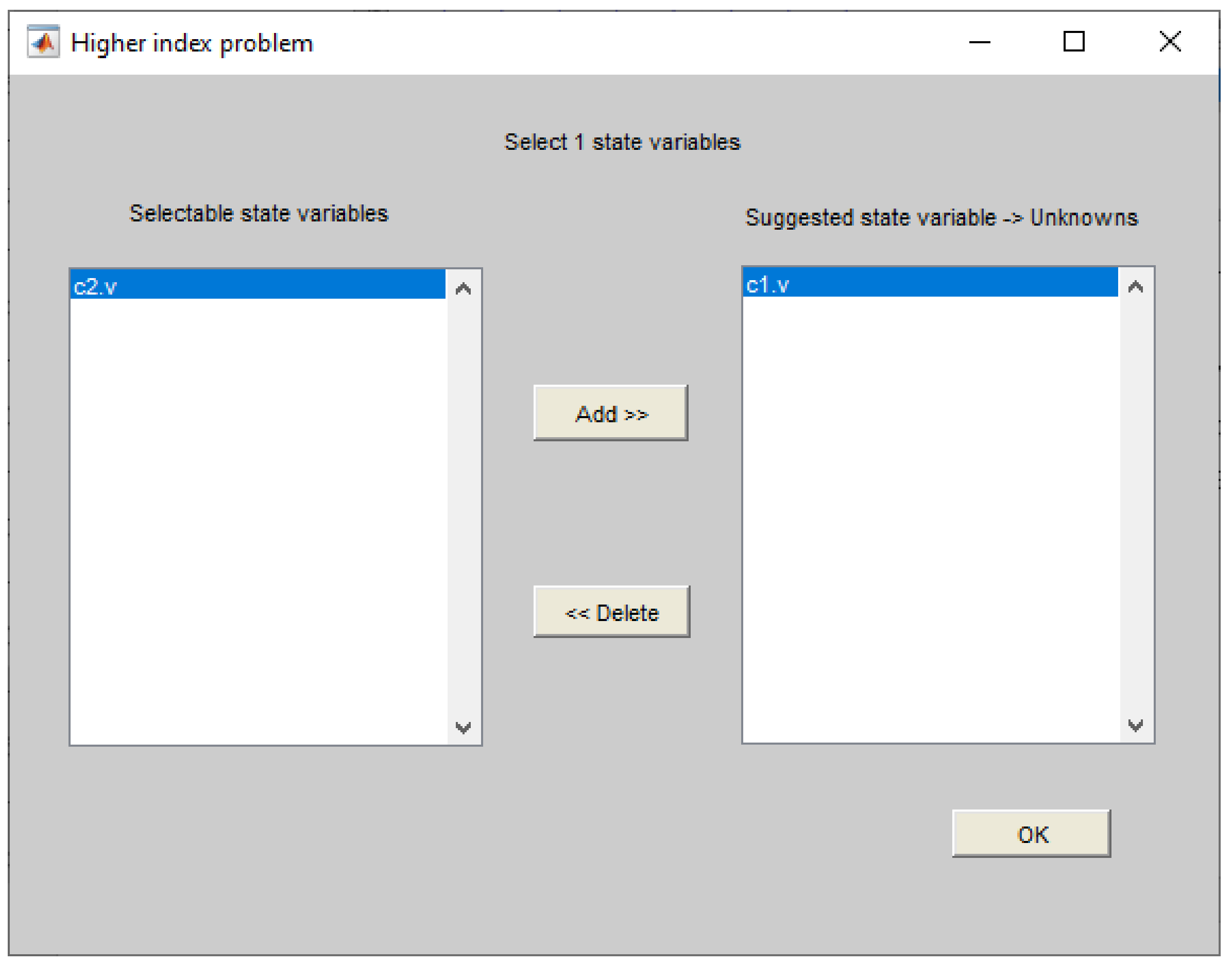
Applying Pantelides’ algorithm, symbolic derivatives with respect to time of singular equations are added to the system, and OOMUCO displays an assistant asking the user to select which state variables should become unknowns and showing which of them are suggested (Figure 20).
With the default selection of state variables in Figure 20, the final sorted incidence matrix shows an algebraic loop (Figure 21), so the system index has been reduced to 1.

4.4. Events

In this example, the motion of a ball bouncing between two walls will be modelled and simulated, considering negligible friction and movement only on the x-axis. OOMUCO’s code for this example is shown in Source code 5, where discrete equations are enclosed within a WHEN clause, which defines the set of conditions for the impact with one wall or another (x < x0 or x > x1). The “reinit” sentences set the new initial conditions both for position and speed to go on the continuous integration after the event processing. Simulation results for 20 seconds are shown in Figure 22.
Source code 5. OOMUCO’s code for bouncing ball example
model rebound
parameter Real x0 = 0 “Left wall”;
parameter Real x1 = 10 “Right wall”;
 Real x(start=8) “Initial ball position”;
 Real vx(start=2) “Initial ball speed”;
equations
 // Model dynamic equations (two state variables)
 der(x) = vx;
 der(vx) = 0;
 // Events
when x < x0 then
  reinit(x,x0);
  reinit(vx,-vx);
elsewhen x > x1 then
  reinit(x,x1);
  reinit(vx,-vx);
end when;
end rebound;
As can be observed from Figure 22, ball position x ranges between values 0 and 10, so the ball is rebounding over time between the left and right walls, respectively. When a rebound occurs, integration stops; the when clause is activated, and the reinit sentence sign changes the current ball speed vx and assigns value x1 or x0 (depending on the wall) to x. Then, integration resumes using the new values of the state variables.

5. Evaluation

One of the main goals of the proposed tool was to improve student learning of OOM key concepts and algorithms, supplementing theoretical explanations. Therefore, OOMUCO was used in a modelling and simulation course of the Automatic Control and Industrial Electronics Engineering degree at University of Cordoba. There is an specific subject devoted to OOM in this course, which covers the following topics: introduction to OOM and its core concepts, description of OOM languages’ main characteristics and use, introduction to DAE and how they arise in OOM, how partition generation is carried out and typical issues related with it (equation sorting, computational causality, algebraic loops, overdetermined systems, etc.) and description of algorithms used in the previous steps. These theoretical concepts are explained to the students in several lectures.
Once the theory was covered, OOMUCO was presented. Firstly, language sentences and structures implemented in the tool for system modelling were described and, after that, its components (compiler, simulator, etc.) and workflow (model creation with the integrated OOM language, partition generation and steps for simulation) were explained. Then, some typical examples included in the tool were described (introduced in Section 4), taking all necessary steps with OOMUCO to obtain a final executable model and the subsequent simulation. These examples are study cases which cover the different issues that may arise when OOM paradigm is applied to system modelling (algebraic loops, higher index systems, etc.). By doing so, the students can learn the basic concepts of the OOM paradigm, how to create models using an OOM language and understand how the different algorithms for partition generation work. Further examples included in the tool were suggested to be reviewed individually by the students for better undestanding.
In addition, the students had to complete a couple of homework exercises prepared for using OOMUCO from model creation to final simulation and to write a detailed explanatory report where they had to analyse the obtained results. The steps involved in each exercise were:
  • Modelling of each case applying the OOM paradigm and the built-in OOM language included in the tool. It was encouraged to use typical features such as ports, abstract or generic components, inheritance, etc.
  • Partition generation, noticing the different incidence matrices and equation sets obtained in each step and how the algorithms automatically solve the computational causality assignment and the potential issues that may arise.
  • Simulation of the final executable model, testing different parameter values and state variables’ initial conditions.

5.1. Student Survey of the Tool

After completing their practical work, students were asked to complete a voluntary questionnaire, using an online platform to gather their opinions (Table 1) based on those used in similar surveys [34,63,64]. Included questions were classified into three categories: improvement in learning, teaching support and usability of the tool.
  • Improvement in learning questions consider the students’ opinions as to whether the tool has helped them to learn the OOM’s theoretical concepts and to create models using OOM languages.
  • Teaching support questions evaluate if the tool is useful as a complement to lecture classes.
  • Usability of the tool questions allow to know, from the student’s point of view, if the tool’s GUI is clear and easy to use and if the workflow is intuitive and the information provided by the tool is easy to interpret.
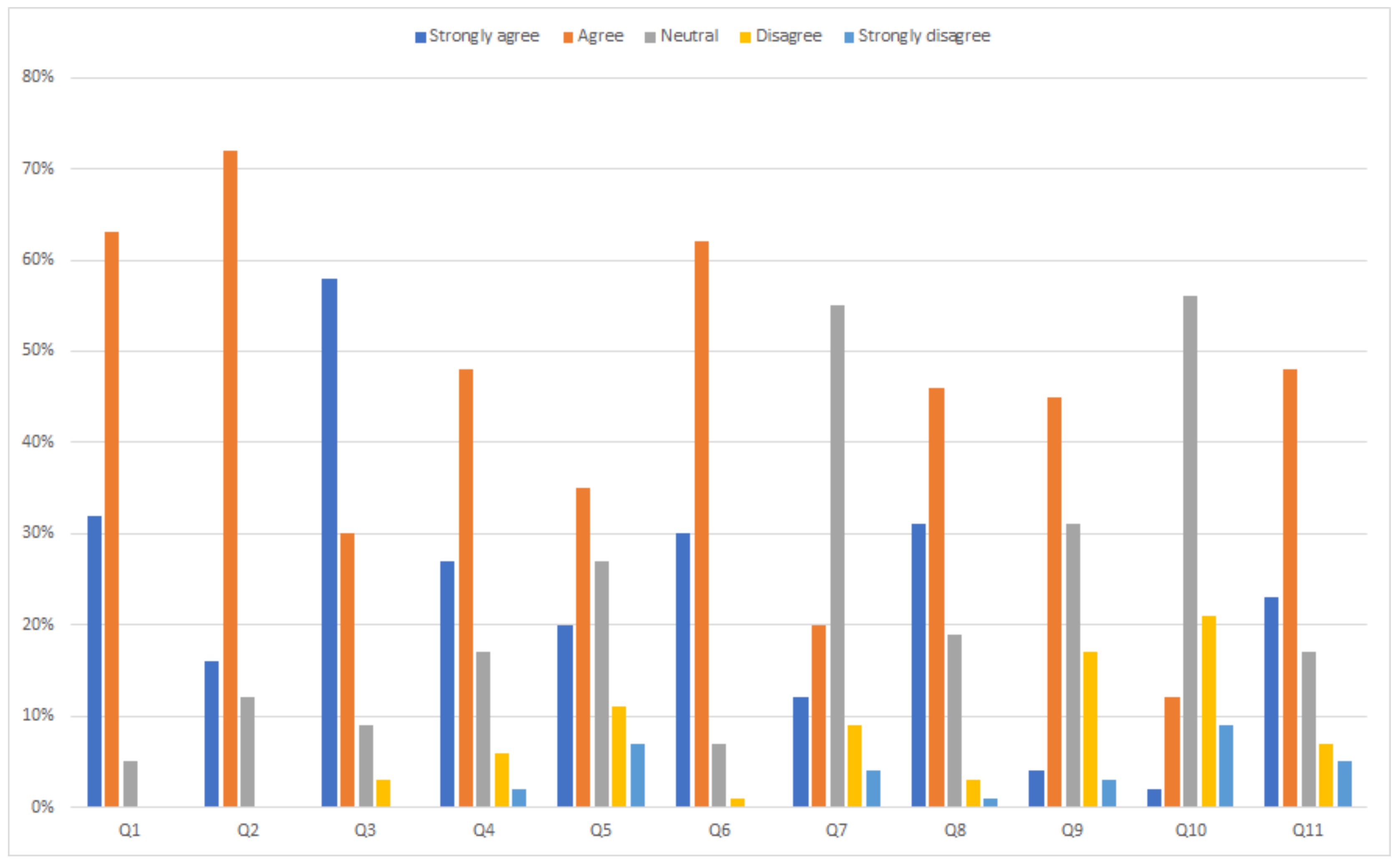
Table 2 summarizes and Figure 23 details, respectively, the students’ answers (22 students were surveyed), which were rated as Strongly agree, Agree, Neutral, Disagree and Strongly disagree using a Likert scale. It is observed that, in the Learning value category, response rates for Strongly agree and Agree are fairly high, so the students find the tool useful both to learn and consolidate the OOM concepts and to practice model creation using that paradigm. In the Teaching support category, although response rate for Agree is the highest and for Strongly agree is not low, it can be seen a higher rate for Neutral than expected, remarkably affected by answers to question Q7. This implies that, according to students’ opinion, additional examples included in the tool are not as significant complement to teaching as those selected for lectures or homework exercises, which have been highly valued. On the other hand, higher rates for Neutral and Disagree are observed in the Usability and easy understanding of the tool category compared to those in the other two. The students think the OOM concepts are presented clearly by the tool, and its workflow is easy to follow (question Q11), but the GUI, though easy to understand and use (question Q9), could be more user-friendly (question Q10).
Previous analysis suggests a good acceptance from the students to use the tool, although it will be necessary to slightly improve the GUI and include other additional exercises. Moreover, current course has been the first one in which the tool has been introduced, so the authors think its integration with subject contents will be improved, and student acceptance will be raised in future courses.

5.2. Student Assessment

As commented before, the students had to do a couple of practical homework exercises using the tool, covering the contents taught in class and whose complexity was similar to the examples described in Section 4. Each exercise was a case study about model creation of a physical system using the OOM paradigm, generation of an executable equation set and its simulation. Firstly, each student had to decompose the global system into its components, creating an “object” hierarchy, and define their models from their dyamic equations, discrete behaviour and their connection “ports”. Then, such models and connections with each other had to be implemented using the OOM language included into OOMUCO to obtain the whole model. Once it had been created, partition generation had to be carried out using the tool, noting the equation processing and the successive incidence matrices obtained after applying the required algorithms. Finally, different simulations of the executable model had to be done, changing values of parameters and state variables’ initial conditions. The students had to analyse the effect of these changes in simulation and relate them with the physical behaviour of the real system.
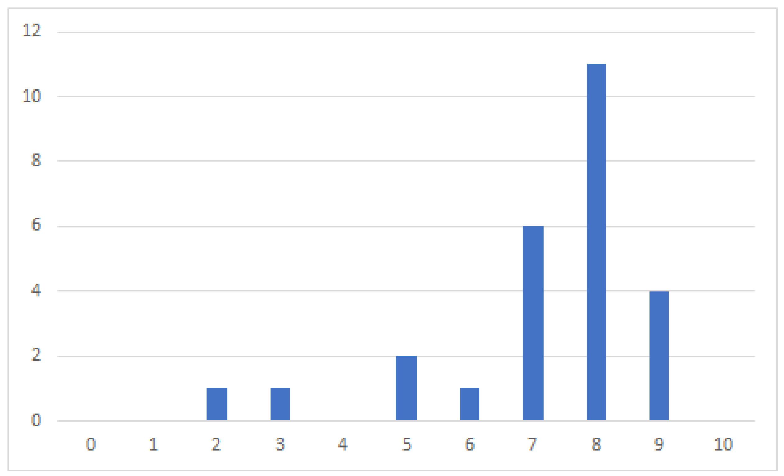
All the students of the current academic year (26 students), none of them with prior background on OOM, submitted via the online learning platform of the University of Cordoba [65] an individual explanatory report with their solution to the exercises. Figure 24 shows the students’ mark distribution with an average of 7.19 and a rate of passing students of 92.31%. It seems clear that the vast majority of the students successfully solved the proposed exercises using the tool and, therefore, largely learned the OOM concepts taught in class.
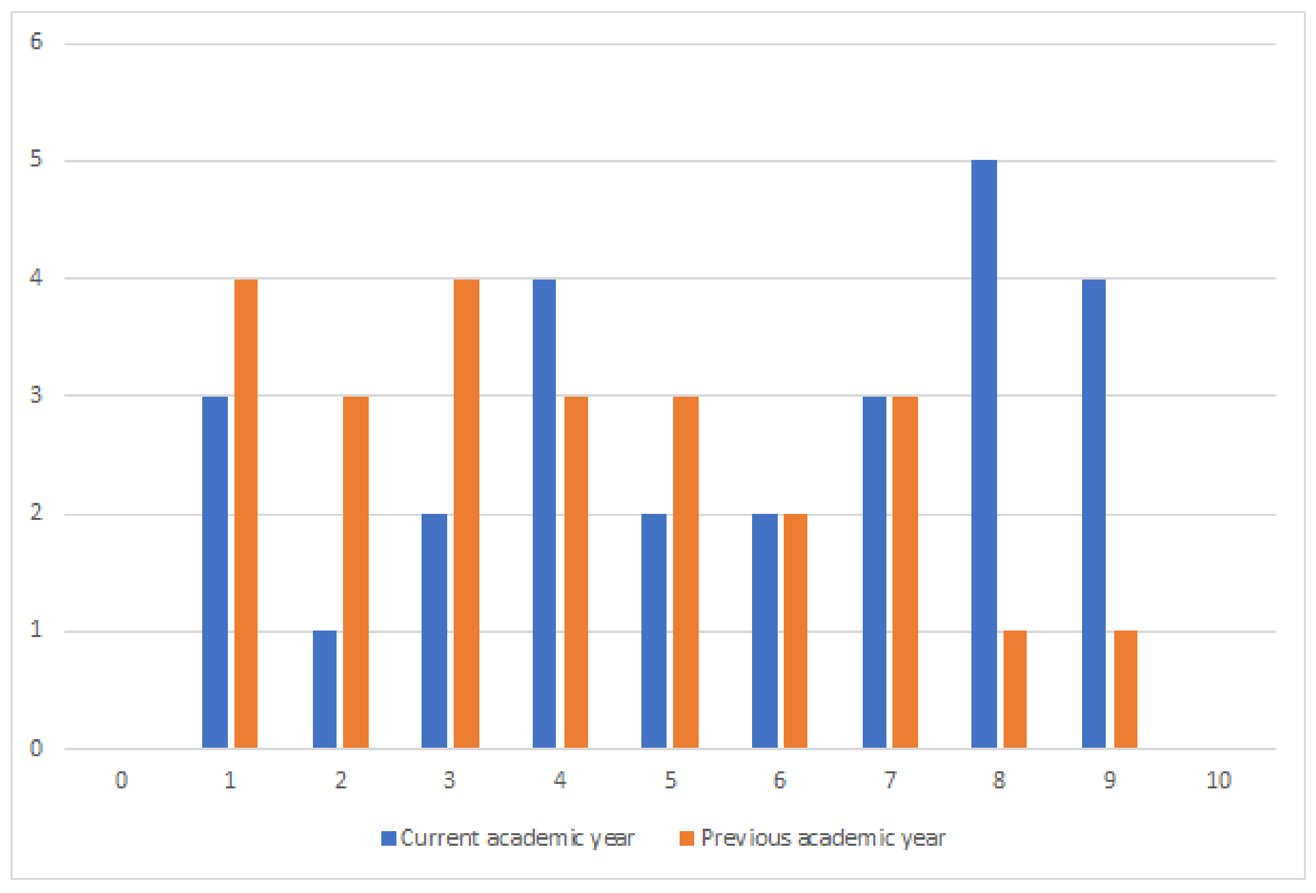
Additionaly, both in the current and previous academic years, all the students also had to take a final exam (24 students in the previous one). This consisted on several brief theory questions about the OOM paradigm and a short practical modelling exercise. As previously stated, only the current students used OOMUCO. Figure 25 shows the students’ marks in the current academic year and in the previous one, and Figure 26 shows the rates of passing and failing students in both years. The average mark of current and previous academic years was 5.62 and 4.13, respectively, so the improvement is noticeable. In addition, a remarkable increase in the percentage of passing students between current and previous years can be observed. Therefore, it seems clear that there has been an important enhancement in learning of the OOM concepts in the academic year where the tool has been introduced.

6. Conclusions

In this paper, a software tool focused on Object-Oriented Modelling (OOM) has been presented. It allows to create models using a built-in OOM language which includes the paradigm’s typical features such as encapsulation of behaviour (continuous and discrete equations and clauses) with its associated data in classes, connections (ports), abstract models or inheritance. It also implements different algorithms for automatic partition generation and allows the simulation of the final equation set. The tool can be used both to teach theoretical and practical foundations of OOM and partition generation algorithms and to create and simulate models of real systems. Student feedback shows that the tool has been a satisfactory complement to lectures, improving their understanding and learning about OOM. Nevertheless, the student survey carried out suggests that the usability of the tool should be enhanced, specifically the GUI, which could be more user-friendly. Additionaly, student assessment clearly shows that the average mark in the current academic year (in which the tool has been introduced) has been improved compared with that in the previous one, as well as the rate of passing students respect to failing ones. Therefore, it can be concluded that the use of the tool has had a substantial beneficial effect on learning OOM concepts.

Author Contributions

Conceptualization, A.B. and F.V.; software, A.B., F.V. and J.J.; validation and formal analysis, J.J., J.G. and M.L.R.; writing-original draft preparation, J.J.

Funding

This research received no external funding.

Conflicts of Interest

The authors declare no conflict of interest.

References

  1. Cellier, F.E. Continuous System Modeling; Springer Science & Business Media: New York, USA, 1991; pp. 1–756. [Google Scholar]
  2. Elmqvist, H.; Cellier, F.E.; Otter, M. Object-oriented modeling of hybrid systems, 1993; pp. 31–41.
  3. Cellier, F.E. Object-oriented modeling: Means for dealing with system complexity. In Proceedings of the 15th Benelux Meeting on Systems and Control, Mierlo, The Netherlands, 6–8 March 1996; pp. 53–64. [Google Scholar]
  4. Fritzson, P. Principles of Object-Oriented Modeling and Simulation with Modelica 3.3: A Cyber-Physical Approach; John Wiley & Sons: Hoboken, NJ, USA, 2014. [Google Scholar]
  5. Cellier, F.E.; Elmqvist, H. Automated formula manipulation supports object-oriented continuous-system modeling. IEEE Control Syst. Mag. 1993, 13, 28–38. [Google Scholar] [Green Version]
  6. Cellier, F.E.; Kofman, E. Continuous System Simulation; Springer Science & Business Media: New York, USA, 2006; pp. 1–644. [Google Scholar]
  7. The Modelica Association—Modelica Association. Available online: https://www.modelica.org/ (accessed on 3 August 2019).
  8. Dymola-Dassault Systèmes®. Available online: https://www.3ds.com/products-services/catia/products/dymola/ (accessed on 3 August 2019).
  9. Modeling and Simulation of Technical Systems ESI ITI. Available online: https://www.simulationx.com/ (accessed on 3 August 2019).
  10. Welcome to Open Modelica. Available online: https://openmodelica.org/ (accessed on 3 August 2019).
  11. MapleSim-Advanced System-Level Modeling & Simulation-Maplesoft. Available online: https://www.maplesoft.com/products/maplesim/ (accessed on 3 August 2019).
  12. PSE: Products-gPROMS-Home. Available online: https://www.psenterprise.com/products/gproms (accessed on 3 August 2019).
  13. E.A. International. EcosimPro, Modelling and Simulation Software. Available online: https://www.ecosimpro.com/products/ecosimpro/ (accessed on 3 August 2019).
  14. Vázquez, F.; Jiménez, J.; Garrido, J.; Belmonte, A. Introduction to Modelling and Simulation with EcosimPro; Prentice Hall: Madrid, Spain, 2010; pp. 1–260. [Google Scholar]
  15. Zhao, L.; Coplien, J. Understanding symmetry in object-oriented languages. J. Object Technol. 2003, 2, 123–134. [Google Scholar] [CrossRef]
  16. Hamza, G.; Hammadi, M.; Barkallah, M.; Choley, J.-Y.; Riviere, A.; Louati, J.; Haddar, M. Analytical based approach for vibration analysis in modelica: Application to the bridge crane system. Appl. Cond. Monit. 2019, 13, 83–91. [Google Scholar]
  17. Al Ashi, M.M.; Elaydi, H.; Abu Hadrous, I. Modelica Based Object-Oriented Modeling and PD-Computed Torque Control of a 2-DOF Robotic Arm. In Proceedings of the International Conference on Promising Electronic Technologies (ICPET), Deir El-Balah, Palestinian Authority, 3–4 October 2018; pp. 13–18. [Google Scholar]
  18. Meinel, D.; Rast, S.; Franke, J. A simulation framework for theoretical analysis and virtual testing of longitudinal vibrations of trains. In Proceedings of the 2nd International Conference on Mechatronics Systems and Control Engineering, New York, NY, USA, 21–23 February 2018; Volume 2018, pp. 38–44. [Google Scholar]
  19. Dominguez-Jimenez, J.A.; Campillo, J. Object-oriented mathematical modeling for estimating electric vehicle’s range using modelica. Commun. Comput. Inf. Sci. 2018, 885, 444–458. [Google Scholar]
  20. Casella, F.; Bartolini, A.G.; Leva, A. Equation-Based Object-Oriented modelling and simulation of large-scale Smart Grids with Modelica. IFAC-PapersOnLine 2017, 50, 5542–5547. [Google Scholar] [CrossRef]
  21. Tillmanns, D.; Gertig, C.; Schilling, J.; Gibelhaus, A.; Bau, U.; Lanzerath, F.; Bardow, A. Integrated design of ORC process and working fluid using PC-SAFT and Modelica. Energy Procedia 2017, 129, 97–104. [Google Scholar] [CrossRef]
  22. Fu, Y.; Zuo, W.; Wetter, M.; VanGilder, J.W.; Yang, P. Equation-based object-oriented modeling and simulation of data center cooling systems. Energy Build. 2019, 198, 503–519. [Google Scholar] [CrossRef] [Green Version]
  23. Carballo, J.A.; Bonilla, J.; Berenguel, M.; Palenzuela, P. Parabolic trough collector field dynamic model: Validation, energetic and exergetic analyses. Appl. Therm. Eng. 2019, 148, 777–786. [Google Scholar] [CrossRef]
  24. Zhou, G.; Ye, Y.; Zuo, W.; Zhou, X.; Wu, X. Fast and efficient prediction of finned-tube heat exchanger performance using wet-dry transformation method with nominal data. Appl. Therm. Eng. 2018, 145, 133–146. [Google Scholar] [CrossRef]
  25. Ali, M.; Vukovic, V.; Muhammad Ali, H.; Ahmed Sheikh, N. Performance Analysis of Solar-Assisted Desiccant Cooling System Cycles in World Climate Zones. J. Sol. Energy Eng. Trans. ASME 2018, 140, 041009. [Google Scholar] [CrossRef]
  26. Dong, X.; Ma, R. Simulation of the solar cell production amorphous silicon thin-film solar cell production system. AIP Conf. Proc. 2019, 2122, 020051. [Google Scholar]
  27. Müller, R.; Kiam, J.J.; Mothes, F. Multiphysical simulation of a semi-autonomous solar powered high altitude pseudo-satellite. In Proceedings of the IEEE Aerospace Conference, Big Sky, MT, USA, 3–10 March 2018; Volume 2018, pp. 1–16. [Google Scholar]
  28. Casella, F.; Parini, P. Optimal Control of Power Generation Systems using Realistic Object-Oriented Modelica Models. IFAC-PapersOnLine 2017, 50, 11100–11106. [Google Scholar] [CrossRef]
  29. Garrido, J.; Zafra, A.; Vázquez, F. Object oriented modelling and simulation of hydropower plants with run-of-river scheme: A new simulation tool. Simul. Model. Pract. Theory 2009, 17, 1748–1767. [Google Scholar] [CrossRef]
  30. Martin-Villalba, C.; Urquia, A.; Shao, G. Implementations of the Tennessee Eastman Process in Modelica. IFAC-PapersOnLine 2018, 51, 619–624. [Google Scholar] [CrossRef]
  31. Carballo, J.A.; Bonilla, J.; Roca, L.; de la Calle, A.; Palenzuela, P.; Berenguel, M. Optimal operating conditions analysis of a multi-effect distillation plant. Desalin. Water Treat. 2017, 69, 229–235. [Google Scholar] [CrossRef]
  32. Garrido, J.; Ruz, M.; Morilla, F.; Vázquez, F. Interactive Tool for Frequency Domain Tuning of PID Controllers. Processes 2018, 6, 197. [Google Scholar] [CrossRef]
  33. Ruz, M.; Garrido, J.; Vazquez, F.; Morilla, F. Interactive Tuning Tool of Proportional-Integral Controllers for First Order Plus Time Delay Processes. Symmetry 2018, 10, 569. [Google Scholar] [CrossRef]
  34. Morales, D.C.; Jimenez-Hornero, J.E.; Vazquez, F.; Morilla, F. Educational tool for optimal controller tuning using evolutionary strategies. IEEE Trans. Educ. 2011, 55, 48–57. [Google Scholar] [CrossRef]
  35. Guzmán, J.L.; Hägglund, T.; Aström, K.J.; Dormido, S.; Berenguel, M.; Piguet, Y. Understanding PID design through interactive tools. IFAC Proc. Vol. 2014, 47, 12243–12248. [Google Scholar] [CrossRef] [Green Version]
  36. Ruiz, Á.; Jiménez, J.E.; Sánchez, J.; Dormido, S. Design of event-based PI-P controllers using interactive tools. Control Eng. Pract. 2014, 32, 183–202. [Google Scholar] [CrossRef]
  37. Prada, M.A.; Reguera, P.; Alonso, S.; Morán, A.; Fuertes, J.J.; Domínguez, M. Communication with resource-constrained devices through MQTT for control education. IFAC-PapersOnLine 2016, 49, 150–155. [Google Scholar] [CrossRef]
  38. Meegahapola, L.G.; Thilakarathne, C. Dynamic Learner-Assisted Interactive Learning Tools for Power Systems Engineering Courses. IEEE Trans. Educ. 2019, 62, 149–156. [Google Scholar] [CrossRef]
  39. de Prado, R.P.; García-Cárdenas, M.; García-Galán, S.; Muñoz-Expósito, J.E. Interactive tool for learning propagation in single-mode optical fibers in telecommunication engineering. Comput. Appl. Eng. Educ. 2019, 27, 789–813. [Google Scholar] [CrossRef]
  40. Notaroš, B.M.; McCullough, R.; Manić, S.B.; Maciejewski, A.A. Computer-assisted learning of electromagnetics through MATLAB programming of electromagnetic fields in the creativity thread of an integrated approach to electrical engineering education. Comput. Appl. Eng. Educ. 2019, 27, 271–287. [Google Scholar] [CrossRef]
  41. Huang, J.; Ong, S.K.; Nee, A.Y.-C. An approach for augmented learning of finite element analysis. Comput. Appl. Eng. Educ. 2019, 27, 921–933. [Google Scholar] [CrossRef]
  42. Rangel, R.L.; Martha, L.F. LESM—An object-oriented MATLAB program for structural analysis of linear element models. Comput. Appl. Eng. Educ. 2019, 27, 553–571. [Google Scholar] [CrossRef]
  43. García-Oliver, J.M.; García, A.; de la Morena, J.; Monsalve-Serrano, J. Teaching combustion thermochemistry with an interactive Matlab application. Comput. Appl. Eng. Educ. 2019, 27, 642–652. [Google Scholar] [CrossRef]
  44. Gamo, J. Assessing a Virtual Laboratory in Optics as a Complement to On-Site Teaching. IEEE Trans. Educ. 2019, 62, 119–126. [Google Scholar] [CrossRef]
  45. Dogmus, Z.; Erdem, E.; Patoglu, V. ReAct!: An interactive educational tool for AI planning for robotics. IEEE Trans. Educ. 2015, 58, 15–24. [Google Scholar] [CrossRef]
  46. Biegler, L.T. Differential-algebraic equations (DAEs). Lect. Notes 2000, 1–40. [Google Scholar]
  47. Brenan, K.E.; Campbell, S.L.; Petzold, L.R. Numerical Solution of Initial-Value Problems in Differential-Algebraic Equations; SIAM: Philadelphia, PA, USA, 1996; Volume 14. [Google Scholar]
  48. Belmonte, A.; Garrido, J.; Jiménez, J.E.; Vázquez, F. Recomputing causality assignments on lumped process models when adding new simplification assumptions. Symmetry 2018, 10, 102. [Google Scholar] [CrossRef]
  49. Duff, I.S.; Erisman, A.M.; Reid, J.K. Direct Methods for Sparse Matrices; Oxford University Press: Oxford, UK, 2017. [Google Scholar]
  50. Dulmage, A.L.; Mendelsohn, N.S. Coverings of bipartite graphs. Can. J. Math. 1958, 10, 517–534. [Google Scholar] [CrossRef]
  51. Duff, I.S. On algorithms for obtaining a maximum transversal. ACM Trans. Math. Softw. 1981, 7, 315–330. [Google Scholar] [CrossRef]
  52. Duff, I.S.; Reid, J.K. An implementation of Tarjan’s algorithm for the block triangularization of a matrix. ACM Trans. Math. Softw. 1978, 4, 137–147. [Google Scholar] [CrossRef]
  53. Elmqvist, H.; Otter, M. Methods for tearing systems of equations in object-oriented modeling. In Proceedings of the European Simulation and Modelling Conference, Barcelona, Spain, 1–3 June 1994; Volume 94, pp. 1–3. [Google Scholar]
  54. Shampine, L.F.; Reichelt, M.W.; Kierzenka, J.A. Solving index-1 DAEs in MATLAB and Simulink. SIAM Rev. 1999, 41, 538–552. [Google Scholar] [CrossRef]
  55. Bujakiewicz, P.; van den Bosch, P.P.J. Determination of perturbation index of a DAE with maximum weighted matching algorithm. In Proceedings of the IEEE Symposium on Computer-Aided Control Systems Design (CACSD), Tucson, AZ, USA, 7–9 March 1994; pp. 129–136. [Google Scholar]
  56. Petzold, L.R. Description of DASSL: A Differential/Algebraic System Solver; Sandia National Labs: Livermore, CA, USA, 1982. [Google Scholar]
  57. Mattsson, S.E.; Söderlind, G. Index reduction in differential-algebraic equations using dummy derivatives. SIAM J. Sci. Comput. 1993, 14, 677–692. [Google Scholar] [CrossRef]
  58. Pantelides, C.C. The consistent initialization of differential-algebraic systems. SIAM J. Sci. Stat. Comput. 1988, 9, 213–231. [Google Scholar] [CrossRef]
  59. Mattsson, S.E.; Soderlind, G. A new technique for solving high-index differential-algebraic equations using dummy derivatives. In Proceedings of the IEEE Symposium on Computer-Aided Control System Design, Napa, CA, USA, 17–19 March 1992; pp. 218–224. [Google Scholar]
  60. Mattsson, S.E.; Olsson, H.; Elmqvist, H. Dynamic selection of states in Dymola. In Proceedings of the Modelica Workshop, Lund, Sweden, 23–24 October 2000; pp. 61–67. [Google Scholar]
  61. MATLAB-MathWorks. Available online: https://www.mathworks.com/products/matlab.html (accessed on 3 August 2019).
  62. Elmqvist, H.; Mattsson, S.E.; Otter, M. Modelica—A language for physical system modeling, visualization and interaction. In Proceedings of the IEEE International Symposium on Computer Aided Control System Design, Kohala Coast, HI, USA, 27 August 1999; pp. 630–639. [Google Scholar]
  63. Dormido, R.; Vargas, H.; Duro, N.; Sánchez, J.; Dormido-Canto, S.; Farias, G.; Esquembre, F.; Dormido, S. Development of a web-based control laboratory for automation technicians: The three-tank system. IEEE Trans. Educ. 2008, 51, 35–44. [Google Scholar] [CrossRef]
  64. Fragoso, S.; Ruz, M.L.; Garrido, J.; Vázquez, F.; Morilla, F. Educational software tool for decoupling control in wind turbines applied to a lab-scale system. Computer Applications in Engineering Education 2016, 24, 400–411. [Google Scholar] [CrossRef] [Green Version]
  65. Moodle Map—Universidad de Córdoba. Available online: http://moodle.uco.es/moodlemap/ (accessed on 5 August 2019).
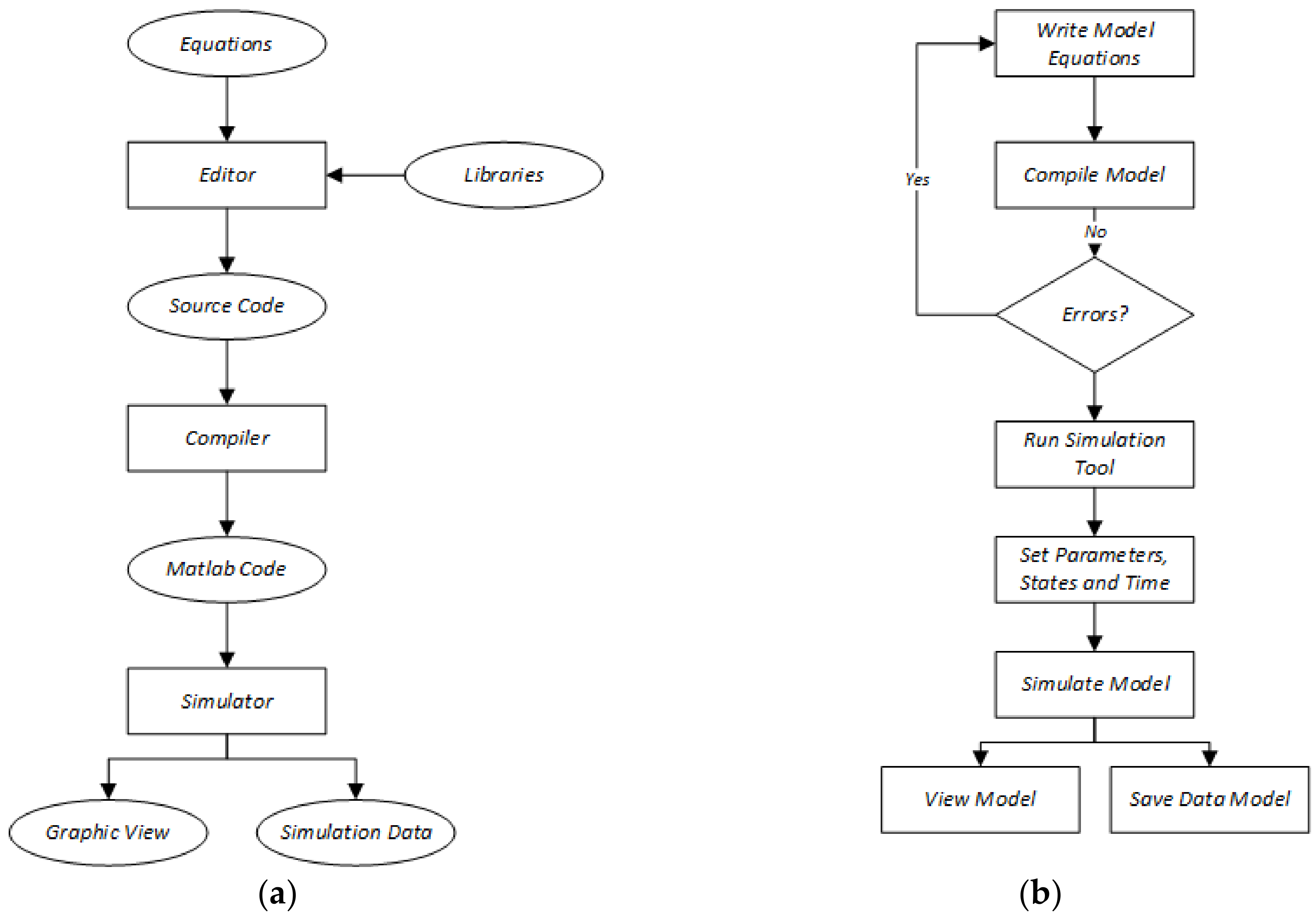
Figure 1. (a) OOMUCO components (editor, compiler and simulator) and tool workflow; (b) simulation steps.
Symmetry 11 01199 g001
Figure 2. Main window with a model file loaded.
Symmetry 11 01199 g002
Figure 3. Options dialog box.
Symmetry 11 01199 g003
Figure 4. Component selection for generating partition.
Symmetry 11 01199 g004
Figure 5. Example of original incidence matrix and equations.
Symmetry 11 01199 g005
Figure 6. Example of final incidence matrix and sorted equations.
Symmetry 11 01199 g006
Figure 7. Simulation window.
Symmetry 11 01199 g007
Figure 8. Example of graphical simulation.
Symmetry 11 01199 g008
Figure 9. Electrical circuit as an example of index-0 DAE.
Symmetry 11 01199 g009
Figure 10. Original incidence matrix (index-0 DAE example).
Symmetry 11 01199 g010
Figure 11. Sorted incidence matrix (index-0 DAE example).
Symmetry 11 01199 g011
Figure 12. Simulation results (index-0 DAE example).
Symmetry 11 01199 g012
Figure 13. Original incidence matrix (linear algebraic loop example).
Symmetry 11 01199 g013
Figure 14. Sorted incidence matrix (linear algebraic loop example).
Symmetry 11 01199 g014
Figure 15. Simulation results (linear algebraic loop example).
Symmetry 11 01199 g015
Figure 16. Electrical circuit with two capacitors in parallel (higher index system).
Symmetry 11 01199 g016
Figure 17. Initial incidence matrix (two capacitors in parallel example).
Symmetry 11 01199 g017
Figure 18. Sorted incidence matrix (two capacitors in parallel example).
Symmetry 11 01199 g018
Figure 19. First sorted incidence matrix (two capacitors in parallel example modelled with the OOM paradigm).
Symmetry 11 01199 g019
Figure 20. OOMUCO’s higher index problem assistant (two capacitors in parallel example modelled with the OOM paradigm).
Symmetry 11 01199 g020
Figure 21. Final sorted incidence matrix (two capacitors in parallel example modelled with OOM).
Symmetry 11 01199 g021
Figure 22. Simulation of bouncing ball example.
Symmetry 11 01199 g022
Figure 23. Students’ answers to the tool survey (22 students).
Symmetry 11 01199 g023
Figure 24. Students’ marks distribution in the homework exercises.
Symmetry 11 01199 g024
Figure 25. Students’ marks distribution in current and previous academic years.
Symmetry 11 01199 g025
Figure 26. (a) Rate of passing and failing students in the current academic year and (b) in the previous one.
Symmetry 11 01199 g026
Table 1. Questionnaire for tool survey.
Improvement in Learning
Q1Did the tool help you to understand and learn the OOM paradigm’s key concepts?
Q2Do you think the tool has improved your skills to create mathematical models using OOM languages?
Q3Did the tool make it easy for you to remember the theoretical concepts taught in lectures?
Q4Rate if using the tool has motivated you in learning the OOM paradigm
Teaching Support
Q5Did the tool help you to understand how the partition generation algorithms work?
Q6Have tool examples used in lectures been helpful to improve your learning?
Q7Rate the additional examples included in the tool
Q8Were homework exercises using the tool useful to strengthen your ability to create and simulate models according to OOM paradigm?
Usability and Easy Understanding of the Tool
Q9Do you think the tool is easy to understand and use?
Q10Do you think the tool’s GUI is intuitive and user-friendly?
Q11Are the workflow and the concepts presented in the tool clear and easy to follow?
Table 2. Response rates in each category.
CategoriesStrongly AgreeAgreeNeutralDisagreeStrongly Disagree
Learning value (Q1–Q4)33%53%11%2%1%
Teaching Support (Q5–Q8)23%41%27%6%3%
Usability and easy understanding of the tool (Q9–Q11)10%35%35%15%4%