Distribution-Based Approaches to Deriving Weights from Dual Hesitant Fuzzy Information

Abstract

Modern cognitive psychologists believe that the decision act of cognitive bias on decision results is universal. To reduce their negative effect on dual hesitant fuzzy decision-making, we propose three weighting methods based on distribution characteristics of data. The main ideas are to assign higher weights to the mid arguments considered to be fair and lower weights to the ones on the edges regarded as the biased ones. The means and the variances of the dual hesitant fuzzy elements (DHFEs) are put forward to describe the importance degrees of the arguments. After that, these results are expanded to deal with the hesitant fuzzy information and some examples are given to show their feasibilities and validities.

1. Introduction

In real life, there is a tremendous amount of uncertain information which is hard to describe in mathematical form directly. For example, a man with a height of 1.75 m is tall or not, an apple is ripe or not. To depict these epistemic uncertainties, the concept of fuzzy set (FS) [1] was proposed in 1965, and soon attracted widespread attention. Now, it has been extended to several expression forms, such as the intuitionistic fuzzy set (IFS) [2], the hesitant fuzzy set (HFS) [3], and the dual hesitant fuzzy set (DHFS) [4]. The IFS is composed of the membership information, non-membership information, and hesitancy information to express imprecise human cognitions of affirmation, negation, and hesitation. However, it is known that if one value is powerless to express the membership information comprehensively, then the HFS [3] overcomes this shortcoming. It allows the decision-makers to provide more membership degrees for reflecting their natural consideration as much as possible when they are hesitant. Furthermore, considering the limitation of the IFS and the HFS, the dual hesitant fuzzy set (DHFS) [4], which is composed of the sets of membership degrees and the sets of non-membership degrees, was proposed to model the uncertain information. Among these sets, the DHFS can be seen as a more comprehensive set, and the other sets, including the FS, IFS and HFS, can be taken as the special cases of the DHFS in some circumstances [4].

At present, the research related to the DHFSs has achieved great progress in these aspects: (1) several foundational concepts are introduced. As the most basic units, the addition, multiplication, exponentiation, and other operations were defined [4,5] first. Then, the most commonly used measures and indexes were proposed, i.e., the correlation coefficient [6], distance measures [7,8], entropy [9], and cross-entropy measures [10], etc. (2) Some valuable decision-making methods were developed. Liang [11] used the ideas of three-way decisions to solve the dual hesitant fuzzy decision-making problems. Based on the correctional score function and the dice similarity measure, Ren and Wei [12] developed a prioritized multi-attribute decision-making method for solving dual hesitant fuzzy problems. When dealing with group decision-making problems, two methods [13] based on the Choquet integral and Shapley index are workable. (3) The DHFS was extended. Although the DHFS is valid enough to depict several kinds of decision-making problems, its expression ability is limited on certain cases. So, by integrating rough set theory, the dual hesitant fuzzy rough set (DHFRS) [14] was obtained. To evaluate the constructional engineering software quality, Xu and Wei [15] introduced the dual hesitant bipolar fuzzy set (DHBFS) and the corresponding aggregation operators were derived.

In the decision-making process, how to acquire the weight information of the attributes is recognized as a key issue. In general, these situations that most people encounter can be divided into two categories: (1) the weight information is completely unknown [16,17,18,19,20,21]. In this case, the weights are given relying on the criteria which are set in advance. For example, if the criteria are that the bigger the entropy values of the fuzzy information, the smaller the weights are, then the attributes with bigger entropy values will be assigned smaller weights [17,18,19]. In the same way, the criteria also can be set by the distance to the ideal points [20] and the group consensus [21], etc. (2) The weight information is partly known. Since some constraints were provided ahead, the typical solution is to establish mathematical optimization models whose preference information was obtained from the decision-makers [22,23,24,25]. To date, the research on the weighting methods for DHFSs is limited. All the related methods can be concluded as the solutions relying on the optimization models combining the grey relational analysis theory [24] and the correlation coefficient [25]. However, these models are not available for all cases, so several novel and specialized methods are necessary.

Cognitive bias [26] is a flaw in judgment which is caused by various reasons including the information shortcuts, noisy information, emotional and moral motivations etc. [26,27]. As a common phenomenon to all human beings, it creates uncertainty which creates more trouble in decision-making. Now, we consider a real situation which always occurs in such fields as job interviews, or competitive races: if the decision-makers give their opinions in the form of the DHFSs, and the weight information is completely unknown, how can one make an impartial decision which is less influenced by the cognitive bias? It is worth noting that even though the DHFSs can describe the epistemic uncertain information efficiently, they are weak in modeling the aleatory uncertainty which is always implied in the decision-makers’ opinions [28]. Therefore, the probability theory which is known as an excellent theory to describe the aleatory uncertainty, in terms of the statistical uncertainty, should be given more attention.

Probability, which is the measure of the likelihood that a random phenomenon will occur, has been widely applied in such areas as medical diagnosis, and machine learning to solve various problems [29]. In fuzzy theory, it can be used to determine the weight vectors and the related methods can be mainly divided into two categories: (1) fusing the immediate probability [30] into the aggregation process. The immediate probability which was first introduced by Yager et al. [30], was treated as a part of the aggregation operator. Soon afterwards, the corresponding extensions were proposed respectively, such as the immediate probability-fuzzy OWA (IP-FOWA) operator [31], the probabilistic weighted average (PWA) operator [32] and the probabilistic OWA (POWA) operator [33]; (2) Combining the character of the probability distributions. In this category, the statistical law which exists in the random phenomenon is taken into consideration. Xu [34] used the discrete normal distribution [29] to reduce the negative effect of some biased data on the decision results in real-number situations. Sadiq and Tesfamariam [35] gave a sufficient analysis on exponential distribution-based weighting methods. Furthermore, these developed methods are available for several other types of fuzzy information [36].

Motivated by the above-mentioned weighting methods, we aim to import the probability information to relieve the impact of cognitive bias in dual hesitant fuzzy decision-making problems. The remainder of this paper is organized as follows: Section 2 recalls some basic concepts and aggregation operators corresponding to dual hesitant fuzzy elements (DHFEs). In Section 3, we develop some weighting approaches based on derivations with dual hesitant fuzzy information, and then we expand them to give weights to hesitant fuzzy elements (HFEs) [37]. In Section 4, some typical examples for DHFEs and HFEs are presented. Section 5 ends the paper with some conclusions.

2. Preliminaries

In this section, some basic concepts of the DHFSs (or DHFEs) are briefly reviewed as follows:

(1) The concepts of DHFSs and DHFEs.

Let X be a fixed set, then a DHFS D on X is described as $D=\left\{<x,h\left(x\right),g\left(x\right)>|x\in X\right\}$, in which $h\left(x\right)$ and $g\left(x\right)$ are two sets of some values in [0, 1], denoting the possible membership degrees and non-membership degrees of the element $x\in X$ to the set D respectively, with the conditions: $0\le \gamma ,$ $\eta \le 1$, $0\le {\gamma }^{+}+{\eta }^{+}\le 1,$ where $\gamma \in h\left(x\right)$, ${\gamma }^{+}\in h^{+}\left(x\right)$, ${\gamma }^{+}={\displaystyle {\cup }_{\gamma \in h\left(x\right)}\max \left\{\gamma \right\}},$ and ${\eta }^{+}\in g^{+}\left(x\right)$, ${\eta }^{+}={\displaystyle {\cup }_{\eta \in g\left(x\right)}\max \left\{\eta \right\}}$ for all $x\in X$. For convenience, the pair $d\left(x\right)=\left(h\left(x\right),g\left(x\right)\right)$ is called a dual hesitant fuzzy element (DHFE) denoted by $d=\left(h,g\right)$ [4].

(2) The basic aggregation operators.

(i)

A dual hesitant fuzzy weighted averaging (DHFWA) operator of the dimension $n$ is a mapping DHFWA: ${\Omega }^n\to \Omega$, which has an associated $n-$ dimensional vector $w=(w_1,w_2,\cdots ,w_n)$, with $w_i>0,$ $i=1,2,\cdots ,n$ and ${\displaystyle {\sum }_{i=1}^n{w}_i}=1$, such that

$$\mathrm{DHFW}{\mathrm{A}}_w\left(d_1,d_2,\cdots ,d_n\right)=\underset{i=1}{\overset{n}{\oplus }}\left(w_i{d}_i\right)={\displaystyle {\cup }_{{\gamma }_i\in h_i,{\eta }_j\in g_j}\left\{\left\{1-{\displaystyle \prod _{i=1}^n{\left(1-{\gamma }_i\right)}^{w_i}}\right\},\left\{{\displaystyle \prod _{i=1}^n{\left({\eta }_i\right)}^{w_i}}\right\}\right\}}$$

(1)

where $\Omega$ is the set of DHFEs, and $d_1,d_2,\cdots ,d_n$ are a collection of arguments in $\Omega$ [5].

(ii)

A dual hesitant fuzzy weighted geometric (DHFWG) operator of the dimension $n$ is a mapping DHFWG: ${\Omega }^n\to \Omega$, which has an associated $n-$ dimensional vector $w=(w_1,w_2,\cdots ,w_n)$, with $w_i>0,$ $i=1,2,\cdots ,n$ and ${\displaystyle {\sum }_{i=1}^n{w}_i}=1$, such that

$$\mathrm{DHFW}{\mathrm{G}}_w\left(d_1,d_2,\cdots ,d_n\right)=\underset{i=1}{\overset{n}{\otimes }}{\left(d_i\right)}^{w_i}={\displaystyle {\cup }_{{\gamma }_i\in h_i,{\eta }_j\in g_j}\left\{\left\{{\displaystyle \prod _{i=1}^n{\left({\gamma }_i\right)}^{w_i}}\right\},\left\{1-{\displaystyle \prod _{i=1}^n{\left(1-{\eta }_i\right)}^{w_i}}\right\}\right\}}$$

(2)

where $\Omega$ is the set of DHFEs, and $d_1,d_2,\cdots ,d_n$ are a collection of arguments in $\Omega$ [5].

(3) The score function and comparison laws of DHFEs [4].

Let $d_i=\left(h_{d_i}\left(x\right),g_{d_i}\left(x\right)\right)\left(i=1,2\right)$ be any two DHFEs, $s_{d_i}=\frac{1}{l_{h\left(i\right)}}{\displaystyle \sum _{j=1}^{l_{h\left(i\right)}}{h}_{d_i}\left(x_i\right)}-\frac{1}{l_{g\left(i\right)}}{\displaystyle \sum _{j=1}^{l_{g\left(i\right)}}{g}_{d_i}^{}\left(x_i\right)}\left(i=1,2\right)$ the score function of $d_i\left(i=1,2\right)$, and $p_{d_i}=\frac{1}{l_{h\left(i\right)}}{\displaystyle \sum _{j=1}^{l_{h\left(i\right)}}{h}_{d_i}^{}\left(x_i\right)}+\frac{1}{l_{g\left(i\right)}}{\displaystyle \sum _{j=1}^{l_{g\left(i\right)}}{g}_{d_i}^{}\left(x_i\right)} \left(i=1,2\right)$ the accuracy function of $d_i\left(i=1,2\right)$, where $l_{h\left(i\right)}$ and $l_{g\left(i\right)}$ are the numbers of the elements in h and g, respectively, then

(i)

if $s_{d_1}>s_{d_2}$, then $d_1$ is superior to $d_2$, denoted by $d_1\succ d_2$;

(ii)

if $s_{d_1}=s_{d_2}$, then

(a)

if $p_{d_1}=p_{d_2}$, then $d_1$ is equivalent to $d_2$, denoted by $d_1\sim d_2$;

(b)

if $p_{d_1}>p_{d_2}$, then $d_1$ is superior than $d_2$, denoted by $d_1\succ d_2$.

3. Weighting Methods Based on Dual Hesitant Fuzzy Elements (DHFEs)

3.1. The Distance Measures for DHFEs

Although the distance and similarity measures for DHFSs were proposed [37], it is not suitable to describe the relationship between two elements completely. So, in this subsection, our research focuses on the distance and similarity measures for DHFEs.

Definition 1.

Let$d_1$and$d_2$be two DHFEs.$r\left(d_1,d_2\right)$is called the distance measure between$d_1$and$d_2$, if$r\left(d_1,d_2\right)$satisfies the following properties:

(1) 

$0\le r\left(d_1,d_2\right)\le 1$;

(2) 

$r\left(d_1,d_2\right)=0$if and only if$d_1$=$d_2$;

(3) 

$r\left(d_1,d_2\right)=r\left(d_2,d_1\right)$.

Definition 2.

Let$d_1$and$d_2$be two DHFEs.$s\left(d_1,d_2\right)$is said to be the similarity measure between$d_1$and$d_2$, if$s\left(d_1,d_2\right)$satisfies the following properties:

(1) 

$0\le s\left(d_1,d_2\right)\le 1$;

(2) 

$s\left(d_1,d_2\right)=1$if and only if$d_1$=$d_2$;

(3) 

$s\left(d_1,d_2\right)=s\left(d_2,d_1\right)$.

It is same as the other types of fuzzy information [38,39] that $s\left(d_1,d_2\right)=1-r\left(d_1,d_2\right)$. So, when these conclusions in terms of the distance measures are derived, the corresponding similarity measures can be got automatically. If we calculate the distance between two DHFEs $d_1=\left\{h_1\left(x\right),g_1\left(x\right)\right\}$ and $d_2=\{h_2\left(x\right),$ $g_2\left(x\right)\}$, then we let $l_{h_1}$, $l_{h_2}$, $l_{g_1}$ and $l_{g_2}$ be the numbers of values in $h_1\left(x\right)$, $h_2\left(x\right)$, $g_1\left(x\right)$ and $g_2\left(x\right)$, respectively, and $l_h=\max \left\{l_{h_1},l_{h_2}\right\}$, $l_g=\max \left\{l_{g_1},l_{g_2}\right\}$. After that, we need to present the extension methods which were used in the HFSs [39] when $l_{h_1}\ne l_{h_2}$(or $l_{g_1}\ne l_{g_2}$). For example, $h_1\left(x\right)=\{0.2,0.4,0.6\},$ $h_2\left(x\right)=\left\{0.5,0.6\right\}$. It is obvious that $l_{h_1}=3$ and $l_{h_2}=2$ are not equal. Under this situation, $h_2\left(x\right)$ with less membership degree values can be extended to $\{0.5,0.5,0.6\}$ (relying on the pessimistic principle [39]), or be extended to $\left\{0.5,0.6,0.6\right\}$ (relying on the optimistic principle) [39].Then the distance formulas are available for them. Finally, we use the pessimistic principal in the following discussion since it is generally assumed that the decision-makers are pessimistic [39].

On account of the fact that the DHFE can be seen as the special case of the DHFS when there is only one element in the DHFS, so the distance measures with respect to the DHFEs can be derived from the distance measures of the DHFSs directly. Thus, below we propose the basic distance formulas for the DHFEs:

(1)

The dual hesitant normalized Hamming distance between two DHFEs $d_1$ and $d_2$:

$$r_{dhnh}(d_1,d_2)=\frac{1}{2l_h}{\displaystyle \sum _{j=1}^{l_h}\left|h_1^{\sigma \left(j\right)}\left(x\right)-h_2^{\sigma \left(j\right)}\left(x\right)\right|}+\frac{1}{2l_g}{\displaystyle \sum _{j=1}^{l_g}\left|g_1^{\sigma \left(j\right)}\left(x\right)-g_2^{\sigma \left(j\right)}\left(x\right)\right|}$$

(3)

(2)

The dual hesitant normalized Euclidean distance between two DHFEs $d_1$ and $d_2$:

$$r_{dhne}(d_1,d_2)={\left[\frac{1}{2l_h}{\displaystyle \sum _{j=1}^{l_h}{\left|h_1^{\sigma \left(j\right)}\left(x\right)-h_2^{\sigma \left(j\right)}\left(x\right)\right|}^2}+\frac{1}{2l_g}{\displaystyle \sum _{j=1}^{l_g}{\left|g_1^{\sigma \left(j\right)}\left(x\right)-g_2^{\sigma \left(j\right)}\left(x\right)\right|}^2}\right]}^{\raisebox{1ex}{$1$}\!\left/ \!\raisebox{-1ex}{$2$}\right.}$$

(4)

(3)

The dual hesitant normalized Hamming–Hausdorff distance between two DHFEs $d_1$ and $d_2$:

$$r_{dhnhh}(d_1,d_2)=\max \left\{\underset{j}{\max }\left|h_1^{\sigma \left(j\right)}\left(x\right)-h_2^{\sigma \left(j\right)}\left(x\right)\right|,\underset{k}{\max }\left|g_1^{\sigma \left(k\right)}\left(x\right)-g_2^{\sigma \left(k\right)}\left(x\right)\right|\right\}$$

(5)

where $h_i^{\sigma \left(j\right)}\left(x\right)$ and $g_i^{\sigma \left(j\right)}\left(x\right)\left(i=1,2\right)$ are the jth largest values in $h_i\left(x\right)$ and $g_i\left(x\right)$, respectively. Moreover, we will give the definitions of the mean (mid one) and the standard deviation (the divergence degree) of a collection of the DHFEs $d_i\left(i=1,2,\cdots ,n\right)$ as follows:

Definition 3.

Let$d_i=\left(h_i,g_i\right)$($i=1,2,\cdots ,n$) be a collection of DHFEs, then we call$\overline{d}=\left(\overline{h},\overline{g}\right)$the mean of these DHFEs, where$\overline{h}=\left\{{\overline{h}}_{}^{\sigma \left(j\right)}|j=1,2,\cdots ,l_h\right\}$,$\overline{g}=\left\{{\overline{g}}_{}^{\sigma \left(k\right)}|k=1,2,\cdots ,l_g\right\},$and

$${\overline{h}}_{}^{\sigma \left(j\right)}=\frac{1}{n}{\displaystyle \sum _{i=1}^n{h}_i^{\sigma \left(j\right)}},{\overline{g}}_{}^{\sigma \left(k\right)}=\frac{1}{n}{\displaystyle \sum _{i=1}^n{g}_i^{\sigma \left(k\right)}}$$

(6)

where${\overline{h}}_{}^{\sigma \left(j\right)}\left(x\right)$is the jth largest values in$\overline{h}\left(x\right)$; while${\overline{g}}_{}^{\sigma \left(k\right)}\left(x\right)$is the kth largest values in$\overline{g}\left(x\right)$.$l_h$is the maximal number of the values in$h_i$($i=1,2,\cdots ,n$); while$l_g$is the maximal number of values in$g_i$($i=1,2,\cdots ,n$).

Remark 1.

If the numbers of the values in$h_i$(or$g_i$) ($i=1,2,\cdots ,n$) are not the same, we can extend the shorter one by the pessimistic principle (or the optimistic principle) [39] as described in Section 2. For example, assume that$d_1=\{\left\{0.6,0.4,0.3\right\}, \left\{0.2,0.1\right\}\}$and$d_2=\{\left\{0.5,0.4,\right\},\{0.4,0.3,0.2,0.1\left\}\right\}$are two DHFEs. To get the means of$d_1$and$d_2$, they should be extended, and the extension form are shown below:

$$d_1{}^{\prime }=\left\{\left\{0.6,0.4,0.3\right\},\left\{0.2,0.1,0.1,0.1\right\}\right\}, d_2{}^{\prime }=\left\{\left\{0.5,0.4,0.4\right\},\left\{0.4,0.3,0.2,0.1\right\}\right\}$$

then the means of$d_1$and$d_2$can be computed as follows:

$$\begin{array}{ll}\overline{d}& =\left\{\left\{\frac{0.6+0.5}{2},\frac{0.4+0.4}{2},\frac{0.3+0.4}{2}\right\},\left\{\frac{0.2+0.4}{2},\frac{0.1+0.3}{2},\frac{0.1+0.2}{2},\frac{0.1+0.1}{2}\right\}\right\}\\ & =\left\{\left\{0.55,0.4,0.35\right\},\left\{0.3,0.2,0.15,0.1\right\}\right\}\end{array}$$

Remark 2.

Let$d_1,d_2,\cdots ,d_n$be a collection of DHFEs, and$d_1{}^{\prime },d_2{}^{\prime },\cdots ,d_n{}^{\prime }$be their extension forms, respectively. Then,$s_{\overline{d}}$(which is the score of the mean$\overline{d}$of the DHFEs$d_1,d_2,\cdots ,d_n$) is also the mean of the scores of the collection of$d_1{}^{\prime },d_2{}^{\prime },\cdots ,d_n{}^{\prime }$.

Proof. 

Let ${\overline{h}}_{}^{\sigma \left(j\right)}=\frac{1}{n}{\displaystyle \sum _{i=1}^n{h}_i^{\sigma \left(j\right)}}$ and ${\overline{g}}_{}^{\sigma \left(k\right)}=\frac{1}{n}{\displaystyle \sum _{i=1}^n{g}_i^{\sigma \left(k\right)}}$, then

$$\begin{gathered} s_{\overline{d}}={\displaystyle \sum _{j=1}^{l_h}\left({\overline{h}}^{\sigma \left(j\right)}\right)}-{\displaystyle \sum _{k=1}^{l_g}\left({\overline{g}}^{\sigma \left(k\right)}\right)}={\displaystyle \sum _{j=1}^{l_h}\left(\frac{1}{n}{\displaystyle \sum _{i=1}^n{h}_i^{\sigma \left(j\right)}}\right)}-{\displaystyle \sum _{k=1}^{l_g}\left(\frac{1}{n}{\displaystyle \sum _{i=1}^n{g}_i^{\sigma \left(k\right)}}\right)} \\ =\frac{1}{n}{\displaystyle \sum _{j=1}^{l_h}{\displaystyle \sum _{i=1}^n{h}_i^{\sigma \left(j\right)}}}-\frac{1}{n}{\displaystyle \sum _{k=1}^{l_g}{\displaystyle \sum _{i=1}^n{g}_i^{\sigma \left(k\right)}}}=\frac{1}{n}{\displaystyle \sum _{i=1}^n\left({\displaystyle \sum _{j=1}^{l_h}{h}_i^{\sigma \left(j\right)}}-{\displaystyle \sum _{k=1}^{l_g}{g}_i^{\sigma \left(k\right)}}\right)}=\frac{1}{n}{\displaystyle \sum _{i=1}^n{s}_{d_i^{\prime }}}. \end{gathered}$$

 □

Based on Remark 2, it is clear that $s_{\overline{d}}$ is almost the same as the mean of the score of the collection of $d_1,d_2,\cdots ,d_n$. Furthermore, the standard deviation is useful in describing the characteristics of DHFEs, so we will give the following definition:

Definition 4.

Let$d_1,d_2,\cdots ,d_n$be a collection of DHFEs, where$d_i=\left(h_i,g_i\right)$,$i=1,2,\cdots ,n$, and let$\overline{d}=\left(\overline{h},\overline{g}\right)$be the mean of these DHFEs, then the standard deviation of these DHFEs can be defined as:

$$\sigma =\sqrt{\frac{1}{n}{\displaystyle \sum _{i=1}^n{r}^2\left(d_i,\overline{d}\right)}}$$

(7)

where$r\left(d_i,\overline{d}\right)$represents the distance between the means$\overline{d}$and$d_i$.

3.2. Three Weighting Methods Based on DHFEs

In this section, specific analysis and the corresponding solutions for the question that how to make an impartial decision to reduce the influence of cognitive bias will be presented.

Modern cognitive psychologists believe that decision results are very susceptible to cognitive bias and their influences are universal in the decision-making process [27]. Here we take the job interview for example: suppose that there are n decision-makers who come from different fields, i.e., the management position, the professional technical post, human resource management, etc. Due to their different knowledge backgrounds, different starting points, and different physical and mental conditions, it is inevitable that there will be some cognitive biases in the opinions provided by the decision-makers. If these n scores (arguments) for one interviewee provided by them are in the number form, and they are arranged in ascending order on the number axis, then the most common case is that majority numbers (representing the majority’s opinions) are similar which are always in the center and only minority numbers (always deviating from other’s opinion) which are too high or too low on the edges. As a kind of familiar random phenomenon, the statistical law implied in it is always depicted by the normal distributions which is often applied in the natural and social sciences to represent real-valued random variables whose distributions are not known. In light of the $3\sigma$ principle [29] derived from the normal distribution, the center data are always recognized as reliable data with less bias [29].

Hence, a feasible solution to reduce the negative impacts of the cognitive bias is to adjust the weights allocation with respect to their positions that the weight is the biggest for center arguments and gradually becomes lower toward the edge. When the decision-makers’ opinions are expressed in the comprehensive forms of the DHFEs $d_1,d_2,\cdots ,d_n$. Firstly, we should find out the mid one (the mean of DHFEs) $\overline{d}$, then we assign the weights to the DHFEs $d_i\left(i=1,2,\cdots ,n\right)$ based on the distances between $d_i$ and $\overline{d}$ $\left(i=1,2,\cdots ,n\right)$. The bigger the distance values, the lower weights assign to them. In the light of these principles, the values of $1-r\left(d_i,\overline{d}\right)$ are proportional to the weights $d_i$, $i=1,2,\cdots ,n$. So, we can define the weights of $d_i\left(i=1,2,\cdots ,n\right)$ as:

$$w_i^{(1)}=\frac{1-r\left(d_i,\overline{d}\right)}{{\displaystyle \sum _{j=1}^n\left(1-r\left(d_j,\overline{d}\right)\right)}}, i=1,2,\cdots ,n$$

(8)

which can also be rewritten as:

$$w_i^{(1)}=\frac{s\left(d_i,\overline{d}\right)}{{\displaystyle \sum _{j=1}^{n}s\left(d_j,\overline{d}\right)}}, i=1,2,\cdots ,n$$

(9)

Because $1-r\left(d_i,\overline{d}\right)$ is a linear function, the method using Equation (8) or Equation (9) are called weighting methods based on the linear functions.

Besides the linear functions, the inverse functions are suitable to reveal the relationship between the distance and the weight that the bigger the distance values $r\left(d_i,\overline{d}\right)\left(i=1,2,\cdots ,n\right)$ are, the smaller the values of $\frac{1}{r\left(d_i,\overline{d}\right)}$ are. Hence, we can assign the weights for the DHFEs $d_i\left(i=1,2,\cdots ,n\right)$ as follows:

$$w_i^{(2)}=\frac{\frac{1}{r\left(d_i,\overline{d}\right)}}{{\displaystyle \sum _{j=1}^n\frac{1}{r\left(d_j,\overline{d}\right)}}}, i=1,2,\cdots ,n$$

(10)

which are called weighting methods based on the inverse function.

In addition, the normal distribution can be discretized to depict the data distribution [40]. Let $x$ be a continuous random variable, and its probability density function [29] can be defined as:

$$f(x)=\frac{1}{\sqrt{2\pi }\sigma }{e}^{-\frac{{(x-\mu )}^2}{2{\sigma }^2}},\hspace{1em}-\infty <x<+\infty$$

(11)

where $\mu$ and $\sigma$($\sigma >0$) are two constants. Then $x$ is normally distributed with a mean ($\mu$) and a standard deviation ($\sigma$).

In Equation (11), the formula ${\left(x-\mu \right)}^2$ can be seen as the square of the distance between the variable value $x$ and the mean $\mu$. So it is reasonable for us to substitute $x-\mu$ into $r\left(d_i,\overline{d}\right)\left(i=1,2,\cdots ,n\right)$ for the representation of the importance of the DHFEs $d_i\left(i=1,2,\cdots ,n\right)$. Therefore, another weighting formula for DHFEs can be derived:

$$w_i^{(3^{\prime })}=\frac{1}{\sqrt{2\pi }\sigma }{e}^{-\frac{r^2\left(d_i,\overline{d}\right)}{2{\sigma }^2}}, i=2,\cdots ,n$$

(12)

whose normalized form is:

$$w_i^{(3)}=\frac{\frac{1}{\sqrt{2\pi }\sigma }{e}^{-\frac{r^2\left(d_i,\overline{d}\right)}{2{\sigma }^2}}}{{\displaystyle \sum _{j=1}^n\frac{1}{\sqrt{2\pi }\sigma }{e}^{-\frac{r^2\left(d_j,\overline{d}\right)}{2{\sigma }^2}}}}=\frac{e^{-\frac{r^2\left(d_i,\overline{d}\right)}{2{\sigma }^2}}}{{\displaystyle \sum _{j=1}^n{e}^{-\frac{r^2\left(d_j,\overline{d}\right)}{2{\sigma }^2}}}}, i=2,\cdots ,n$$

(13)

which can be called the method based on the normal distribution.

To explore some characteristics of the proposed three methods, we assume that the distances $r\left(d_i,\overline{d}\right)\left(i=1,2,\cdots ,n\right)$ are variable, and then $w_i^{(j)}\left(j=1,2,3\right)$ can be seen as multivariate functions. For convenience, the distance measures $r\left(d_i,\overline{d}\right)(i=1,2,\cdots ,n)$ are denoted by $r_i{}^{\prime }$. Afterwards, several conclusions are derived.

Theorem 1.

$w_i^{(j)}(j=1,2,3)$are monotonously decreasing functions with respect to the values of$r_i{}^{\prime }$.

Proof. 

Because the three weighting functions are different, our proof will be composed of the following three parts:

(1) As for

$$w_i^{(1)}=\frac{1-r_i{}^{\prime }}{{\displaystyle \sum _{j=1}^n\left(1-r_j{}^{\prime }\right)}}, i=1,2,\cdots ,n$$

and when the DHFEs are defined, the denominator ${\displaystyle \sum _{j=1}^n\left(1-r_j{}^{\prime }\right)}$ can be seen as a constant. Therefore, from the functions of the numerator $1-r_i{}^{\prime }(i=1,2,\cdots ,n)$, it is obvious that the smaller the values of $r_i{}^{\prime }$, the bigger $w_i^{(1)}$ is. Therefore, $w_i^{(1)}$ is a monotonously decreasing function with respect to the values of $r_i{}^{\prime }$.

(2) Since

$$w_i^{(2)}=\frac{\frac{1}{r_i{}^{\prime }}}{{\displaystyle \sum _{j=1}^n\frac{1}{r_j{}^{\prime }}}}, i=1,2,\cdots ,n$$

The denominator ${\displaystyle \sum _{j=1}^n\frac{1}{r_j{}^{\prime }}}$ is a constant, the functions of the numerator $\frac{1}{r_i{}^{\prime }}(i=1,2,\cdots ,n)$ are monotonously decreasing functions. Therefore, $w_i^{(j)}\left(i=1,2,\cdots ,n\right)$ are monotonously decreasing functions with respect to the values of $r_i{}^{\prime }$.

(3) As for

$$w_i^{(3)}=\frac{e^{-\frac{r_i{{}^{\prime }}^2}{2{\sigma }^2}}}{{\displaystyle \sum _{j=1}^n{e}^{-\frac{r_i{{}^{\prime }}^2}{2{\sigma }^2}}}}, i=2,\cdots ,n$$

It should be paid attention to $r_i{{}^{\prime }}^2$ and $2{\sigma }^2=\frac{2}{n}{\displaystyle \sum _{j=1}^n{r}_j{{}^{\prime }}^2}$ which are both the functions of $r_i{}^{\prime }$.

So

$$\frac{\partial e^{-\frac{r_i{{}^{\prime }}^2}{2{\sigma }^2}}}{\partial r_i{}^{\prime }}=\left(-1\right)e^{-\frac{r_i{{}^{\prime }}^2}{2{\sigma }^2}}\frac{n{r}_i{}^{\prime }\left({\displaystyle \sum _{\begin{array}{c}j=1\\ j\ne i\end{array}}^n{r}_j{{}^{\prime }}^2}\right)}{{\left({\displaystyle \sum _{j=1}^n{r}_j{{}^{\prime }}^2}\right)}^2}$$

For

$$e^{-\frac{r_i{{}^{\prime }}^2}{2{\sigma }^2}}>0, n>0, {\displaystyle \sum _{\begin{array}{c}j=1\\ j\ne i\end{array}}^n{r}_j{{}^{\prime }}^2}>0, {\displaystyle \sum _{j=1}^n{r}_j{{}^{\prime }}^2}>0$$

Therefore,

$$\frac{\partial e^{-\frac{r_i{{}^{\prime }}^2}{2{\sigma }^2}}}{\partial r_i{}^{\prime }}<0$$

In another word, $e^{-\frac{r_i{{}^{\prime }}^2}{2{\sigma }^2}}$ is monotonously decreasing function with respect to the values of $r_i{}^{\prime }$. Furthermore, the denominator ${\displaystyle \sum _{j=1}^n{e}^{-\frac{r_i{{}^{\prime }}^2}{2{\sigma }^2}}}$ is a constant, so $w_i^{(3)}(i=1,2,\cdots ,n)$ are the decreasing function of $r_i{}^{\prime }$.

Because that $w_i^{(j)}\left(j=1,2,3\right)$ are multivariate and discrete, and there are some relationships among $r_i{}^{\prime }\left(i=1,2,\cdots ,n\right)$. It is hard to present some mathematical analysis merely relying on the function, so in Section 4, we will give some comparisons by virtue of some specific DHFEs. □

3.3. The Weighting Methods Based on HFEs

Hesitant fuzzy set [3] allows the decision-makers to give their opinions by several HFEs. Let $X$ be a fixed set, then the HFS A can be represented by a mathematical symbol $A=\left\{<x,h_A\left(x\right)>|x\in X\right\}$, where the HFE $h_A\left(x\right)$ is a set of some values in $[0, 1]$, denoting the possible membership degrees of the element $x\in X$ to the set A [37].

In light of its superior properties to describe the hesitant information, the HFS has attracted a lot of attention and has been extended to more forms for various applications, such as interval hesitant fuzzy set (IHFS) [41], hesitant triangular fuzzy set (HTFS) [42] and necessary and possible hesitant fuzzy set (NPHFS) [43]. When the decisions are made according to the HFS information, Xu and Xia [44] recommended the concepts of entropy and cross-entropy for HFSs to obtain the weights. Xu and Zhang [45] acquired the weights based on the TOPSIS method [46] with incomplete weight information. However, these weighting methods are lack of the consideration of bias information.

According to Zhu et al. [4], when the non-membership degree set $g=\varnothing$, the DHFE reduces to the HFE. Therefore, in this section, we focus on discussing whether these methods for DHFEs will also be available for HFEs or not.

First, referring to Equations (6) and (7), we should give the explanations of the mid one (mean) and the degree of deviation of data (the standard deviation) for HFEs.

Definition 5.

Let$h_1,h_2,\cdots ,h_n$be a collection of HFEs, we define$\overline{h}$as the mean of these HFEs, where$\overline{h}=\left\{{\overline{h}}_{}^{\sigma \left(j\right)}|j=1,2,\cdots ,l_h\right\},$and

$${\overline{h}}_{}^{\sigma \left(j\right)}=\frac{1}{n}{\displaystyle \sum _{i=1}^n{h}_i^{\sigma \left(j\right)}}$$

(14)

where${\overline{h}}_{}^{\sigma \left(j\right)}\left(x\right)$and$h_i^{\sigma \left(j\right)}\left(x\right)$are the jth largest values in$\overline{h}\left(x\right)$and$h_i\left(x\right)$respectively.$l_h$is the maximal number of values in$h_i$,$i=1,2,\cdots ,n$.

Definition 6.

Let$h_1,h_2,\cdots ,h_n$be a collection of HFEs, and$\overline{h}$be the mean of these HFEs, then we define the standard deviation of these HFEs as:

$$\sigma =\sqrt{\frac{1}{n}{\displaystyle \sum _{i=1}^n{r}^2\left(h_i,\overline{h}\right)}}$$

(15)

where$r\left(h_i,\overline{h}\right)$represents the distance between the mean$\overline{h}$and$h_i$.

Secondly, to evaluate the importance of the HFEs, the distance and similarity measures for the HFEs should be presented which are slightly different from the HFSs’ whose essential is the weighted average of the distance and similarity measures for the HFEs. So, the distance and similarity measures for the HFEs should belong to the interval [0, 1]. For convenience, we suppose that there are two HFEs: $A=h_A\left(x\right)$ and $B=h_B\left(x\right)$. Naturally, the pessimistic principle and the optimistic principle [39] are also available in the calculations for the HFEs. Here, we choose the pessimistic principal [39] as before. Let $l_{h_A}$ and $l_{h_B}$ be the numbers of values in $h_A\left(x\right)$ and $h_B\left(x\right)$ respectively, and $l_x=\max \left\{l_{h_A},l_{h_B}\right\}$. Then, in the following, we get three typical distance measures for HFEs based on Equations (3)–(5):

(1)

The hesitant normalized Hamming distance between two HFEs:

$$r_{hnh}(A,B)=\frac{1}{l_x}{\displaystyle \sum _{j=1}^{l_x}{\left|h_A^{\sigma \left(j\right)}\left(x\right)-h_B^{\sigma \left(j\right)}\left(x\right)\right|}^{}}$$

(16)

(2)

The hesitant normalized Euclidean distance between two HFEs:

$$r_{hne}(A,B)={\left[\frac{1}{l_x}{\displaystyle \sum _{j=1}^{l_x}{\left|h_A^{\sigma \left(j\right)}\left(x\right)-h_B^{\sigma \left(j\right)}\left(x\right)\right|}^2}\right]}^{\raisebox{1ex}{$1$}\!\left/ \!\raisebox{-1ex}{$2$}\right.}$$

(17)

(3)

The hesitant normalized Hamming–Hausdorff distance between two HFEs:

$$r_{hnhh}(A,B)=\underset{j}{\max }\left\{\left|h_A^{\sigma \left(j\right)}\left(x\right)-h_B^{\sigma \left(j\right)}\left(x\right)\right|\right\}$$

(18)

Finally, referring to Equations (8), (10) and (13), the weight values for hesitant arguments can be derived. Assume that the hesitant arguments $h_1,h_2,\cdots ,h_n$ are a collection of n preference values. The weights of $h_i\left(i=1,2,\cdots ,n\right)$ are defined as:

$$w_i^{\left(1\right)}=\frac{1-r\left(h_i,\overline{h}\right)}{{\displaystyle \sum _{j=1}^n\left(1-r\left(h_j,\overline{h}\right)\right)}}, i=1,2,\cdots ,n$$

(19)

Equation (19) can also be rewritten as:

$$w_i^{\left(1\right)}=\frac{s\left(h_i,\overline{h}\right)}{{\displaystyle \sum _{j=1}^{n}s\left(h_j,\overline{h}\right)}}, i=1,2,\cdots ,n$$

(20)

and Equation (10) can be updated as:

$$w_i^{\left(2\right)}=\frac{\frac{1}{r\left(h_i,\overline{h}\right)}}{{\displaystyle \sum _{j=1}^n\frac{1}{r\left(h_j,\overline{h}\right)}}}, i=1,2,\cdots ,n$$

(21)

The weights based on the normal distribution are as follows:

$$w_i^{\left(3\right)}=\frac{e^{-\frac{r^2\left(h_i,\overline{h}\right)}{2{\sigma }^2}}}{{\displaystyle \sum _{j=1}^n{e}^{-\frac{r^2\left(h_j,\overline{h}\right)}{2{\sigma }^2}}}}, i=1,2,\cdots ,n$$

(22)

It should be noted that we use the same symbols $w_i^{\left(j\right)}$ for the HFEs and DHFEs because the methods for HFEs can be regarded as a special case of the methods for DHFEs. Furthermore, it is same as Theorem 1 that the smaller the values $r\left(h_i,\overline{h}\right)$ are, the bigger $w_i^{(j)}\left(j=1,2,3\right)$ are.

4. Illustrative Examples

4.1. Illustrative Examples for DHFEs

In this section, we will make some analyses on the differences and similarities of the three weighting methods by using specific DHFEs.

Example 1.

For a decision-making problem, nine experts$d_i\left(i=1,2,\cdots ,9\right)$are invited to evaluate the performance of the employee A for his/her annual work, and the experts’ opinions are expressed in the form of DHFEs as follows:

$$d_1=\left\{\right\{0.5,0.3\}, \{0.4,0.3\left\}\right\}, d_2=\left\{\right\{0.3,0.2\}, \{0.7\left\}\right\}, d_3=\left\{\right\{0.5,0.4\}, \{0.4\left\}\right\}, d_4=\left\{\right\{0.7,0.6\}, \{0.2\left\}\right\}, d_5=\left\{\right\{0.2\}, \{0.8,0.7,0.5\left\}\right\}, d_6=\left\{\right\{0.4,0.3\}, \{0.5\left\}\right\}, d_7=\left\{\right\{0.9,0.5\}, \{0.1\left\}\right\}, d_8=\left\{\right\{0.6,0.5,0.4\}, \{0.4\left\}\right\}, d_9=\left\{\right\{0.8,0.7,0.6\}, \{0.2\left\}\right\}$$

Then, we need to deal with the decision information, and there are two steps for the implementation of the proposed method presented as follows:

Step 1. Calculate the mean $\overline{d}$ and the standard deviation $\sigma$ according to the Euclidean distance Equation(4), respectively: $\overline{d}$ = {{0.544,0.411,0.389}, {0.411,0.389,0.367}}, and $\sigma$ = 0.189.

Step 2. Determine the experts’ weights by using Equations (8), (10) and (13) respectively. Thus, the gained weights for $d_i\left(i=1,2,\cdots ,9\right)$ are listed in

Table 1. The weights $w_i^{\left(j\right)}\left(i=1,2,\cdots ,9;j=1,2,3\right)$ for the DHFEs $d_i\left(i=1,2,\cdots ,9\right)$.

${\mathit{d}}_{\mathit{i}}$	${\mathit{w}}_{\mathit{i}}^{\left(1\right)}(\mathbf{Ranking})$	${\mathit{w}}_{\mathit{i}}^{\left(2\right)}(\mathbf{Ranking})$	${\mathit{w}}_{\mathit{i}}^{\left(3\right)}(\mathbf{Ranking})$
$d_1$	0.123(3)	0.124(3)	0.161(3)
$d_2$	0.097(8)	0.035(8)	0.057(8)
$d_3$	0.130(1)	0.461(1)	0.173(1)
$d_4$	0.108(5)	0.050(5)	0.101(5)
$d_5$	0.096(9)	0.034(9)	0.053(9)
$d_6$	0.118(4)	0.082(4)	0.142(4)
$d_7$	0.099(7)	0.037(7)	0.063(7)
$d_8$	0.127(2)	0.208(2)	0.169(2)
$d_9$	0.103(6)	0.042(6)	0.080(6)

.

From Table 1, it is clear that the weighting strategies of the three methods are similar. They all assign the highest weights to $d_3$ which is the nearest to the mean $\overline{d}$ and assign the lowest weights to $d_5$ which is the furthest one to the mean $\overline{d}$. To get a full understanding of these methods, in the following, some comparisons among them will be shown as follows:

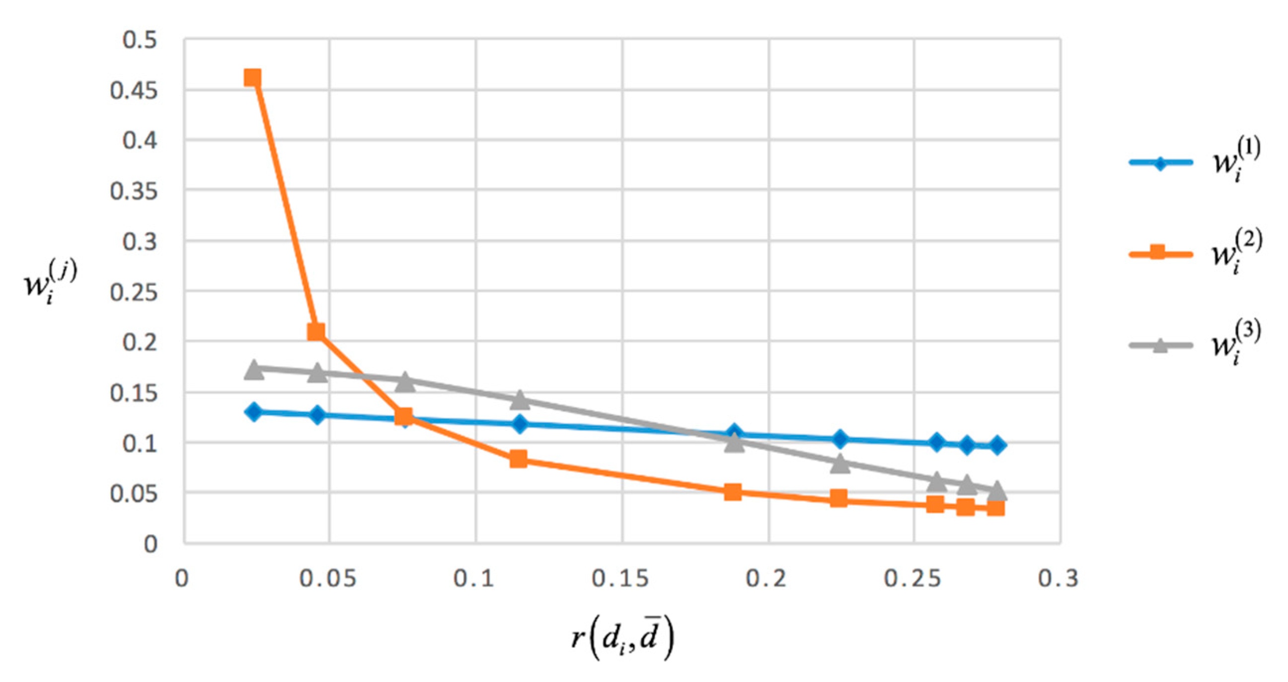
Case 1. Comparisons among the three methods with respect to the distances $r\left(d_i,\overline{d}\right)\left(i=1,2,\cdots ,9\right)$. To provide a clear analysis of them, we put the weights of the DHFEs $d_i\left(i=1,2,\cdots ,9\right)$ obtained from these three proposed methods, respectively, into Figure 1.

From Figure 1, we can find some similarities and differences between the three weighting methods: (1) For all of the three methods, the weights decrease when the distances increase, that is to say, the further the distance between $d_i$ and $\overline{d}$ is, the lower the weight is; (2) It is obvious that the degrees of the divergence of these weights $w_i^{\left(j\right)}\left(j=1,2,3\right)$ derived from different methods are different. Among them, the degree of the divergence of $w_i^{\left(2\right)}\left(i=1,2,\cdots ,9\right)$ is the biggest one and the degree of the divergence of $w_i^{\left(1\right)}\left(i=1,2,\cdots ,9\right)$ is the smallest one, correspondingly, the degree of the divergence of $w_i^{\left(3\right)}\left(i=1,2,\cdots ,9\right)$ derived by Equation(13) is in the middle.

It is also clear from Figure 1 that both the highest weight $w_3^{\left(2\right)}$ = 0.461 and the lowest weight $w_5^{\left(2\right)}$ = 0.034 are obtained by Equation (10). Meanwhile, for $w_i^{\left(1\right)}\left(i=1,2,\cdots ,9\right)$, the highest weight is $w_3^{\left(1\right)}$ = 0.130 and the lowest weight is $w_5^{\left(1\right)}$ = 0.096. The main reason for this difference is that $\frac{1}{r\left(d_i,\overline{d}\right)}\left(i=1,2,\cdots ,9\right)$ are inverse proportional functions which are sensitive to small numbers and $r\left(d_i,\overline{d}\right)\left(i=1,2,\cdots ,9\right)$ are small numbers within 0 and 1. On the contrary, $1-r\left(d_i,\overline{d}\right)\left(i=1,2,\cdots ,9\right)$ are linear functions which are less sensitive to even tiny change. Generally, if you want to emphasize the DHFEs near to the mean (mid one(s)), the method based on the inverse proportional function is available. On the other hand, if you want to emphasize both the whole and some individuals, the method based on the linear function is better.

In the existing literature, a classical weighting method called normal distribution weighting method [36] (for convenience, here we call it Xu’s method), which is designed for the OWA operator primordially, has been widely used for determining the weights. Its main idea that assigns higher weights to the mid one(s) and assigns lower weights to the biased ones is similar to the above three methods. Therefore, in the following, we will take some comparisons among them.

Case 2. Comparisons among the three methods and Xu’s method with respect to the ranking of scores. Since Xu’s method is designed for the OWA operator, then in order to conduct some comparisons, we first rank the DHFEs $d_i\left(i=1,2,\cdots ,9\right)$ based on the technique [4] as follows: $d_7\succ d_9\succ d_4\succ d_8\succ d_3\succ d_1\succ d_6\succ d_2\succ d_5$.

Then, according to Xu’s method, the vector of these DHFEs’ weights is $w$ = (0.051, 0.086, 0.124, 0.156, 0.168, 0.156, 0.124, 0.086, 0.051) relying on the ranking of the scores. Thus, we can describe the relationships among the four weighting methods in Figure 2.

Based on Figure 2, it is clear that the method based on the normal distribution for DHFEs is similar to Xu’s method, for example, the weights assigned by the two methods to the mid one $d_3$ are 0.173 and 0.168 respectively. Furthermore, compared with the three weighting methods, when the number of arguments is known, the weight vector of Xu’s method is certain and its graph is symmetrical, while the weight vectors of our proposed three methods are uncertain and the weights will change a little with the values of the attributes. In general, among the four methods, the graph of the inverse proportional function-based method is the sharpest, and the linear function-based method is the smoothest.

Example 2.

The decision strategy for recruitment interview of product manager. The product manager is a position to discover and guide a product that is valuable, usable, and feasible which is also the main bridge between business, technology, and user experience, especially in technology companies [47]. It is so crucial for an enterprise to choose the right person for this position that his decisions will not only help enterprise to create great wealth but also conciliate the opportunities of scientific development for the enterprise. Normally, the recruitment interview for the right person are done by several decision-makers from different positions. Due to their diversities in knowledge backgrounds, cognitive levels, psychological states, etc., their opinions are susceptible to the cognitive bias, and are always hesitant and vague. In this situation, (1) DHFS is an effective tool for the description of the hesitant and vague data. For example, Sahin and Liu [48] applied the DHFSs to solve the investment decision-making problems, Ren and Wei [12] used the DHFSs to describe the indexes in teacher evaluation system. With the use of the dual hesitant fuzzy information, Liang et al. further developed the three-way Decisions [11]. (2) The distribution-based weighting methods mentioned above will be feasible to reduce the negative effect caused by the biased data. Therefore, in the decision strategy for recruitment interview of product manager, according to the dual hesitant fuzzy data provided by the experts, we can use the distribution-based weighting methods to obtain the weight of each expert, then calculate the final scores of the candidates, and finally get the right person for this position.

Assume that there are five candidates $A_i\left(i=1,2,\cdots ,5\right)$ to be selected, and the decision committee includes four experts from different departments: (1) $p_1$ is from board of directors; (2) $p_2$ is from the technology department; (3) $p_3$ is a product manager from the same level; and (4) $p_4$ is from personal department. The assessments of the five candidates $A_i(i=1,2,\cdots ,5)$ provided by the four experts are in the form of DHFEs $d_{ij}$($i=1,2,\cdots ,5;j=1,2,3,4$) listed in

Table 2. Dual hesitant fuzzy decision matrix.

	${\mathit{p}}_1$	${\mathit{p}}_2$	${\mathit{p}}_3$	${\mathit{p}}_4$
$A_1$	{{0.4,0.3}, {0.5}}	{{0.5,0.4}, {0.4,0.3}}	{{0.3,0.2}, {0.6}}	{{0.5,0.4}, {0.5}}
$A_2$	{{0.6}, {0.4}}	{{0.5,0.2,0.1}, {0.4}}	{{0.2}, {0.8,0.7,0.5}}	{{0.5}, {0.5,0.4}}
$A_3$	{{0.8,0.6}, {0.2}}	{{0.7}, {0.2,0.1}}	{{0.6,0.5,0.4}, {0.4}}	{{0.7,0.6,0.5}, {0.3}}
$A_4$	{{0.8}, {0.1}}	{{0.3,0.2,0.1}, {0.2}}	{{0.6,0.5}, {0.4}}	{{0.6}, {0.4,0.3,0.2}}
$A_5$	{{0.6,0.5}, {0.4}}	{{0.4,0.3,0.2}, {0.5}}	{{0.5,0.4}, {0.2}}	{{0.4,0.3,0.2}, {0.5}}

(i.e., the decision matrix $D={\left(d_{ij}\right)}_{5\times 4}$).

Part 1. Evaluation process to choose the appropriate product manager.

The solving method is presented as follows:

Step 1. Calculating weights. Using the hamming distance in Equation (3), we can get the weights of the experts $p_j\left(j=1,2,3,4\right)$ derived from Equations (8), (10) and (13) respectively as follows:

As shown in

Table 3. The weights $w_j^{(1)}\left(j=1,2,3,4\right)$ for the experts $p_j\left(j=1,2,3,4\right)$.

	${\mathit{p}}_1$	${\mathit{p}}_2$	${\mathit{p}}_3$	${\mathit{p}}_4$
$A_1$	0.264	0.241	0.237	0.258
$A_2$	0.247	0.254	0.233	0.266
$A_3$	0.256	0.244	0.236	0.264
$A_4$	0.229	0.234	0.266	0.271
$A_5$	0.257	0.250	0.243	0.250

,

Table 4. The weights $w_j^{(2)}\left(j=1,2,3,4\right)$ for the experts $p_j\left(j=1,2,3,4\right)$.

	${\mathit{p}}_1$	${\mathit{p}}_2$	${\mathit{p}}_3$	${\mathit{p}}_4$
$A_1$	0.567	0.100	0.090	0.243
$A_2$	0.207	0.251	0.153	0.390
$A_3$	0.244	0.140	0.108	0.507
$A_4$	0.130	0.141	0.324	0.405
$A_5$	0.326	0.241	0.191	0.241

and

Table 5. The weights $w_j^{(3)}\left(j=1,2,3,4\right)$ for the experts $p_j\left(j=1,2,3,4\right)$.

	${\mathit{p}}_1$	${\mathit{p}}_2$	${\mathit{p}}_3$	${\mathit{p}}_4$
$A_1$	0.368	0.167	0.136	0.329
$A_2$	0.233	0.276	0.150	0.341
$A_3$	0.308	0.200	0.128	0.363
$A_4$	0.149	0.172	0.330	0.349
$A_5$	0.312	0.250	0.188	0.250

, these weights of the experts $p_j\left(j=1,2,3,4\right)$ are determined respectively according to the assessed values of the five candidates.

Step 2. Evaluations. We use Equations (1) and (2) to calculate the final scores of the candidates $A_i \left(i=1,2,3,4,5\right)$. For convenience, we assume that $\mathrm{DHFW}{\mathrm{A}}_1$, $\mathrm{DHFW}{\mathrm{A}}_2$ and $\mathrm{DHFW}{\mathrm{A}}_3$ represent the aggregated values obtained by the DHFWA operator using $w_j^{(1)}\left(j=1,2,3,4\right)$, $w_j^{(2)}\left(j=1,2,3,4\right)$ and $w_j^{(3)}\left(j=1,2,3,4\right)$ respectively, and $\mathrm{DHFW}{\mathrm{G}}_1$, $\mathrm{DHFW}{\mathrm{G}}_2$ and $\mathrm{DHFW}{\mathrm{G}}_3$ are obtained by the DHFWG operator using $w_j^{(1)}\left(j=1,2,3,4\right)$, $w_j^{(2)}\left(j=1,2,3,4\right)$ and $w_j^{(3)}\left(j=1,2,3,4\right)$ correspondingly. The results are shown in

Table 6. The aggregation results of the arguments $A_i\left(i=1,2,\cdots ,5\right)$ for DHFEs.

	${\mathit{A}}_1$	${\mathit{A}}_2$	${\mathit{A}}_3$	${\mathit{A}}_4$	${\mathit{A}}_5$
$\mathrm{DHFW}{\mathrm{A}}_1$	−0.095	−0.041	0.399	0.360	0.035
$\mathrm{DHFW}{\mathrm{A}}_2$	−0.110	−0.013	0.387	0.315	0.034
$\mathrm{DHFW}{\mathrm{A}}_3$	−0.091	−0.011	0.414	0.319	0.027
$\mathrm{DHFW}{\mathrm{G}}_1$	−0.132	−0.149	0.349	0.209	−0.032
$\mathrm{DHFW}{\mathrm{G}}_2$	−0.129	−0.105	0.352	0.212	−0.031
$\mathrm{DHFW}{\mathrm{G}}_3$	−0.117	−0.106	0.373	0.202	−0.037

:

According to the ranking results in

Table 7. Rankings of the aggregation results for DHFEs using $w_j^{(i)}\left(i=1,2,3;j=1,2,3,4\right)$.

	$\mathbf{D}\mathbf{H}\mathbf{F}\mathbf{W}{\mathbf{A}}_1$	$\mathbf{D}\mathbf{H}\mathbf{F}\mathbf{W}{\mathbf{A}}_2$	$\mathbf{D}\mathbf{H}\mathbf{F}\mathbf{W}{\mathbf{A}}_3$
Ranking	$A_3\succ A_4\succ A_5\succ A_2\succ A_1$	$A_3\succ A_4\succ A_5\succ A_2\succ A_1$	$A_3\succ A_4\succ A_5\succ A_2\succ A_1$
	$\mathbf{D}\mathbf{H}\mathbf{F}\mathbf{W}{\mathbf{G}}_1$	$\mathbf{D}\mathbf{H}\mathbf{F}\mathbf{W}{\mathbf{G}}_2$	$\mathbf{D}\mathbf{H}\mathbf{F}\mathbf{W}{\mathbf{G}}_3$
Ranking	$A_3\succ A_4\succ A_5\succ A_1\succ A_2$	$A_3\succ A_4\succ A_5\succ A_2\succ A_1$	$A_3\succ A_4\succ A_5\succ A_2\succ A_1$

, it is clear that the candidate $A_3$ is more suitable than others for this enterprise no matter using what weighting method and aggregation operator, meanwhile, the ranking results for the five candidates are similar.

Part 2. Discussion

In this section, we shall analyze the influence of the weighting methods. To do so, we compare the entropy-based method [49] with our distribution-based methods.

(1) General analysis

As is shown in Table 7, the ranking results using the DHFWA operator are the same. Since the same operators are adopted, then the ranking results are greatly influenced by the weight values. Based on Table 3, Table 4 and Table 5, no matter which weight formulas are used, the change trends of the weights are the same. So, we get the same rankings according to the DHFWA operator. However, there is also little difference among the rankings obtained by the DHFWG operator. The main reason is that the DHFWG operator is more sensitive to small numbers between 0 and 1.

(2) Comparative analysis

The traditional entropy method [49] which assigns low weight values to the attributes with high entropies can also be applied in this decision-making problem. So, we make some comparisons between the entropy-based methods [49] and the proposed distribution-based methods.

First, we calculate the entropies for DHFEs in Table 2, and the entropy formula [9] is shown below:

$$E\left(d\left(h\left(x\right),g\left(x\right)\right)\right)=\frac{1}{l}{\displaystyle \sum _{i=1}^l\frac{\left(1-\left|h^{\sigma \left(i\right)}\left(x\right)-g^{\sigma \left(i\right)}\left(x\right)\right|\right)\left(2-h^{\sigma \left(i\right)}\left(x\right)-g^{\sigma \left(i\right)}\left(x\right)\right)}{2}}$$

(23)

What needs to be explained is that if $l_h<l_g$, then we extend $h\left(x\right)$ by repeating its maximum element until it has the same length with $g\left(x\right)$. Conversely, if $l_h>l_g$, then an extension of $g\left(x\right)$ is to repeat its minimum element until it has the same length with $h\left(x\right)$ [9].

Then, we calculate the entropy weights basing on the classical formula shown as:

$$w_j^{\left(4\right)}=\frac{1-E(p_j)}{{\displaystyle \sum _{k=1}^4\left(1-E\left(p_k\right)\right)}},j=1,2,3,4$$

(24)

To distinguish these entropy weights from others, we use the symbol $w_j^{(4)}\left(j=1,2,3,4\right)$ for them which are listed in

Table 8. The weights $w_j^{(4)}\left(j=1,2,3,4\right)$ for the experts $p_j\left(j=1,2,3,4\right)$.

	${\mathit{p}}_1$	${\mathit{p}}_2$	${\mathit{p}}_3$	${\mathit{p}}_4$
$A_1$	0.244	0.219	0.298	0.239
$A_2$	0.265	0.209	0.305	0.222
$A_3$	0.280	0.288	0.195	0.237
$A_4$	0.370	0.112	0.245	0.274
$A_5$	0.264	0.250	0.235	0.250

:

Using the DHFWA operator, the final ranking result in

Table 9. The aggregation results using $w_j^{(4)}\left(j=1,2,3,4\right)$.

	${\mathit{A}}_1$	${\mathit{A}}_2$	${\mathit{A}}_3$	${\mathit{A}}_4$	${\mathit{A}}_5$
$\mathrm{DHFW}{\mathrm{A}}_4$	−0.114	−0.064	0.422	0.453	0.034

. is $A_4\succ A_3\succ A_5\succ A_2\succ A_1$ and $A_4$ is taken for the best person for the product manager position.

Compared with the rankings in Table 7, there are two different decisions for the right person. The main reason is that the entropy-based method focuses on reducing the uncertainty in the decision-making process; however, the distribution-based method aims to relieve the impact of the bias information.

Generally speaking, from the above examples, it can be concluded that the three weighting methods highlighting the mid one(s), which coincide with the majority rule in the real life, are valid for DHFEs. Therefore, in the following, we will explore whether these weighting methods can be extended to accommodate the HFEs.

4.2. Illustrative Examples for HFEs

To detect the validity of our methods for HFEs, we transform the DHFEs in Examples 1 and 2 into HFEs, and then take some comparisons.

Example 3.

In this example, we want to find out whether the proposed weighting methods mentioned before are valid when the opinions of experts are expressed by the HFEs. Therefore, first, we should reduce the DHFEs in Example 1 to HFEs as follows:

$$d_1=\{0.5,0.3\}, d_2=\{0.3,0.2\}, d_3=\{0.5,0.4\}, d_4=\{0.7,0.6\}, d_5=\left\{0.2\right\}, d_6=\left\{\right\{0.4,0.3\}, d_7=\{0.9,0.5\}, d_8=\{0.6,0.5,0.4\}, d_9=\{0.8,0.7,0.6\}$$

Then, following the procedure in Example 1, we get the following steps:

Step 1. Calculate the mean $\overline{d}$ and the variance $\sigma$ of these HFEs:

$$\overline{d}=\{0.544,0.411,0.389\}, \sigma =0.126$$

and the Euclidean distance Equation (16) is adopted.

Step 2. With using Equations (19), (21) and (22), the appropriate weights of $h_i\left(i=1,2,\cdots ,9\right)$ are determined, which are listed in Table 7.

Analyzing

Table 10. The weights $w_i^{\left(j\right)}\left(i=1,2,\cdots ,9;j=1,2,3\right)$ for the HFEs $h_i\left(i=1,2,\cdots ,9\right)$.

${\mathit{h}}_{\mathit{i}}$	${\mathit{w}}_{\mathit{i}}^{\left(1\right)}(\mathbf{Ranking})$	${\mathit{w}}_{\mathit{i}}^{\left(2\right)}(\mathbf{Ranking})$	${\mathit{w}}_{\mathit{i}}^{\left(3\right)}(\mathbf{Ranking})$
$h_1$	0.118(3)	0.121(3)	0.152(3)
$h_2$	0.106(6)	0.048(6)	0.082(6)
$h_3$	0.123(1)	0.463(1)	0.168(1)
$h_4$	0.109(5)	0.056(5)	0.099(5)
$h_5$	0.102(9)	0.041(9)	0.060(9)
$h_6$	0.115(4)	0.089(4)	0.137(4)
$h_7$	0.106(7)	0.047(7)	0.079(7)
$h_8$	0.120(2)	0.172(2)	0.161(2)
$h_9$	0.103(8)	0.041(8)	0.062(8)

, we find that the weighting results for the HFEs are similar to the weighting results for the DHFEs, while they all assign the highest weight to the expert $h_3$ and assign the lowest weight to the expert $h_5$. Moreover, both the highest weight $w_3^{\left(2\right)}$ = 0.463 and the lowest weight $w_5^{\left(2\right)}$ = 0.041 are derived from the method based on the inverse proportional function. However, for the loss of some information, there is also little difference among the methods for the HFEs and the methods for the DHFEs. For example, the ranking of the weights for $h_2$ is the sixth in the methods for HFEs, while it is the eighth in the methods for DHFEs.

Example 4.

We attempt to use the new weighting methods to solve the decision-making problem which is mentioned in Example 2 supposing that the decision-making information is in the form of HFSs. The main process is to obtain the weights of experts using the distribution-based weighting methods, then aggregate these data provided by these experts to calculate the final scores for these candidates. First, the experts’ opinions which are demonstrated with DHFEs should be reduced to HFEs, and then we get the hesitant fuzzy decision matrix as shown in

Table 11. Hesitant fuzzy decision matrix.

	$G_1$	$G_2$	$G_3$	$G_4$
$A_1$	{0.4,0.3}	{0.5,0.4}	{0.3,0.2}	{0.5,0.4}
$A_2$	{0.6}	{0.5,0.2,0.1}	{0.2}	{0.5}
$A_3$	{0.8,0.6}	{0.7}	{0.6,0.5,0.4}	{0.7,0.6,0.5}
$A_4$	{0.8}	{0.3,0.2,0.1}	{0.6,0.5}	{0.6}
$A_5$	{0.6,0.5}	{0.4,0.3,0.2}	{0.5,0.4}	{0.4,0.3,0.2}

.

Because the HFEs which are lack of the non-membership degree information can be seen as the special cases of DHFEs, our discussion will focus on the two aspects as: (1) detecting the effectiveness of the three weighting methods for HFEs, and (2) discussing whether less information will influence the ranking results or not.

Using Equations (19), (21) and (22) and the HFWA operator and the HFWG operator defined in Ref. [29], we can calculate the aggregation results and the rankings of arguments $A_i\left(i=1,2,\cdots ,5\right)$. For convenience, let the $\mathrm{HFW}{\mathrm{A}}_j\left(j=1,2,3\right)$ and the $\mathrm{HFW}{\mathrm{G}}_j\left(j=1,2,3\right)$ be the aggregation values obtained from the HFWA operator and the HFWG operator, using the Hamming distances for HFEs, respectively. In the end, the ranking results which are derived from Ref. [29] are got, as listed in

Table 12. The aggregation results of the candidates $A_i\left(i=1,2,\cdots ,5\right)$ based on the HFEs.

	${\mathit{A}}_1$	${\mathit{A}}_2$	${\mathit{A}}_3$	${\mathit{A}}_4$	${\mathit{A}}_5$
$\mathrm{HFW}{\mathrm{A}}_1$	0.383	0.418	0.641	0.592	0.411
$\mathrm{HFW}{\mathrm{A}}_2$	0.380	0.423	0.634	0.567	0.411
$\mathrm{HFW}{\mathrm{A}}_3$	0.394	0.417	0.652	0.600	0.398
$\mathrm{HFW}{\mathrm{G}}_1$	0.364	0.343	0.617	0.492	0.379
$\mathrm{HFW}{\mathrm{G}}_2$	0.367	0.353	0.617	0.546	0.385
$\mathrm{HFW}{\mathrm{G}}_3$	0.379	0.346	0.632	0.534	0.371

.

With the results in

Table 13. Rankings of the aggregation results for the HFEs using $w_j^{(i)}\left(i=1,2,3;j=1,2,3,4\right)$.

	$\mathbf{H}\mathbf{F}\mathbf{W}{\mathbf{A}}_1$	$\mathbf{H}\mathbf{F}\mathbf{W}{\mathbf{A}}_2$	$\mathbf{H}\mathbf{F}\mathbf{W}{\mathbf{A}}_3$
Ranking	$A_3\succ A_4\succ A_2\succ A_5\succ A_1$	$A_3\succ A_4\succ A_2\succ A_5\succ A_1$	$A_3\succ A_4\succ A_2\succ A_5\succ A_1$
	$\mathbf{H}\mathbf{F}\mathbf{W}{\mathbf{G}}_1$	$\mathbf{H}\mathbf{F}\mathbf{W}{\mathbf{G}}_2$	$\mathbf{H}\mathbf{F}\mathbf{W}{\mathbf{G}}_3$
Ranking	$A_3\succ A_4\succ A_5\succ A_1\succ A_2$	$A_3\succ A_4\succ A_5\succ A_1\succ A_2$	$A_3\succ A_4\succ A_1\succ A_5\succ A_2$

, it is certain that the three weighting methods based on HFEs are valid in decision-making, and the candidate $A_3$ is deemed to be the best choice which is the same as the results in Table 7. Secondly, when the HFWA operator is used, the rankings getting from different weights are coincident. As for the HFWG operator, the ranking results vary with the weight vectors slightly. Finally, compared with the results in Table 7, although they reach an agreement on the right person, the rankings of the other arguments are not the same. The primary reason can be ascribed to the loss of the negation information which always play great role in decision-making.

5. Concluding Remarks

In decision-making problems, there are always some cognitive biases which will affect the final decision results. To reduce the influence of this bias data, a better solution is to assign lower weights to the biased values which are always on the edges, and the typical values which are always in the middle higher weights. Based on this idea, we present three distribution-based weighting methods for DHFEs. The prominent characteristic of the developed methods is that they can reduce the influence of biased data, which obey the majority rule as well in some complex fuzzy situations. Then, the application in the decision strategy for the recruitment interview of a product manager has testified the practicability and the validity of the proposed method. The main contributions of this paper are as follows:

(1)

The mean and the standard deviation of a collection of DHFEs have been first defined to describe the mid one(s) and the divergence degrees of a collection of DHFEs.

(2)

Some distances for DHFEs have been introduced to depict the relationships between the mean and DHFEs.

(3)

Based on the natures of the linear function, the inverse proportion function, and the normal distribution function, three weighting methods for DHFEs have been developed, respectively.

(4)

These weighting methods have been extended to accommodate hesitant fuzzy information.

Meanwhile, there are some limitations in this paper as well. The distribution-based methods to derive the weight values aim to reduce the influence of this biased data. However, there may be a set of unbiased data to deal with. Therefore, other methods such as the traditional entropy method [49] will be suitable in this situation as well.

Further attention should be paid to distribution-based methods. First, we can consider using other probability distribution functions as an alternative. Secondly, we can explore other potential use scenarios of distribution-based decision-making methods, such as project evaluation, performance review and so on.

References

1. Zadeh, L.A. Fuzzy sets, information and Control. Inf. Control 1965, 8, 338–353. [Google Scholar] [CrossRef]
2. Atanassov, K.T. Intuitionistic fuzzy sets. Fuzzy Sets Syst. 1986, 20, 87–96. [Google Scholar] [CrossRef]
3. Torra, V. Hesitant fuzzy sets. Int. J. Intell. Syst. 2010, 25, 529–539. [Google Scholar] [CrossRef]
4. Zhu, B.; Xu, Z.S.; Xia, M.M. Dual hesitant fuzzy sets. J. Appl. Math. 2012, 2012, 1–13. [Google Scholar] [CrossRef]
5. Zhu, B.; Xu, Z.S. Some results for dual hesitant fuzzy sets. J. Intell. Fuzzy Syst. 2014, 26, 1657–1668. [Google Scholar]
6. Tyagi, S.K. Correlation coefficient of dual hesitant fuzzy sets and its applications. Appl. Math. Model. 2015, 39, 7082–7092. [Google Scholar] [CrossRef]
7. Su, Z.; Xu, Z.S.; Liu, H.F.; Liu, S.S. Distance and similarity measures for dual hesitant fuzzy sets and their applications in pattern recognition. J. Intell. Fuzzy Syst. 2015, 29, 731–745. [Google Scholar] [CrossRef]
8. Singh, P. Distance and similarity measures for multiple-attribute decision making with dual hesitant fuzzy sets. Comput. Appl. Math. 2015, 36, 111–126. [Google Scholar] [CrossRef]
9. Zhao, N.; Xu, Z.S. Entropy measures for dual hesitant fuzzy information. In Proceedings of the 2015 Fifth International Conference on Communication Systems and Network Technologies, Gwalior, India, 4–6 April 2015; pp. 1152–1156. [Google Scholar]
10. Ye, J. Cross-entropy of dual hesitant fuzzy sets for multiple attribute decision-making. Int. J. Decis. Support Syst. Technol. 2016, 8, 20–30. [Google Scholar] [CrossRef]
11. Liang, D.C.; Xu, Z.S.; Liu, D. Three-way decisions based on decision-theoretic rough sets with dual hesitant fuzzy information. Inf. Sci. 2017, 396, 127–143. [Google Scholar] [CrossRef]
12. Ren, Z.L.; Wei, C.P. A multi-attribute decision-making method with prioritization relationship and dual hesitant fuzzy decision information. Int. J. Mach. Learn. Cybern. 2017, 8, 755–763. [Google Scholar] [CrossRef]
13. Qu, G.H.; Li, Y.J.; Qu, W.H.; Li, C.H. Some new Shapley dual hesitant fuzzy Choquet aggregation operators and their applications to multiple attribute group decision making-based TOPSIS. J. Intell. Fuzzy Syst. 2017, 33, 2463–2483. [Google Scholar] [CrossRef]
14. Zhang, F.W.; Chen, J.H.; Zhu, Y.H.; Li, J.R.; Li, Q.; Zhuang, Z.Y. A dual hesitant fuzzy rough pattern recognition approach based on deviation theories and its application in urban traffic modes recognition. Symmetry 2017, 9, 262. [Google Scholar] [CrossRef]
15. Xu, X.R.; Wei, G.W. Dual hesitant bipolar fuzzy aggregation operators in multiple attribute decision making. Int. J. Knowl.-Based Intell. Eng. Syst. 2017, 21, 155–164. [Google Scholar] [CrossRef]
16. Xu, Z.S.; Zhao, N. Information fusion for intuitionistic fuzzy decision making: An overview. Inf. Fusion 2016, 28, 10–23. [Google Scholar] [CrossRef]
17. Chen, T.Y.; Li, C.H. Determining objective weights with intuitionistic fuzzy entropy measures: A comparative analysis. Inf. Sci. 2010, 180, 4207–4222. [Google Scholar] [CrossRef]
18. Farhadinia, B. A multiple criteria decision making model with entropy weight in an interval-transformed hesitant fuzzy environment. Cognit. Comput. 2017, 9, 513–525. [Google Scholar] [CrossRef]
19. Park, J.H.; Kwark, H.E.; Kwun, Y.C. Entropy and cross-entropy for generalized hesitant fuzzy information and their use in multiple attribute decision making. Int. J. Intell. Syst. 2017, 32, 266–290. [Google Scholar] [CrossRef]
20. Xu, Z.S. Models for multiple attribute decision making with intuitionistic fuzzy information. Int. J. Uncertain. Fuzz. Knowl.-Based Syst. 2007, 15, 285–297. [Google Scholar] [CrossRef]
21. Xu, Z.S.; Cai, X.Q. Nonlinear optimization models for multiple attribute group decision making with intuitionistic fuzzy information. Int. J. Intell. Syst. 2010, 25, 489–513. [Google Scholar] [CrossRef]
22. Wu, J.Z.; Zhang, Q. Multicriteria decision making method based on intuitionistic fuzzy weighted entropy. Expert Syst. Appl. 2011, 38, 916–922. [Google Scholar] [CrossRef]
23. Lin, Y.; Wang, Y.M.; Chen, S.Q. Hesitant fuzzy multiattribute matching decision making based on regret theory with uncertain weights. Int. J. Fuzzy Syst. 2017, 19, 955–966. [Google Scholar] [CrossRef]
24. Yang, S.H.; Ju, Y.B. A GRA method for investment alternative selection under dual hesitant fuzzy environment with incomplete weight information. J. Intell. Fuzzy Syst. 2015, 28, 1533–1543. [Google Scholar]
25. Chen, Y.F.; Peng, X.D.; Guan, G.H.; Jiang, H.D. Approaches to multiple attribute decision making based on the correlation coefficient with dual hesitant fuzzy information. J. Intell. Fuzzy Syst. 2014, 26, 2547–2556. [Google Scholar]
26. Kahneman, D.; Slovic, P.; Tversky, A. Judgment under Uncertainty: Heuristics and Biases; Cambridge University Press: Cambridge, UK, 1982. [Google Scholar]
27. Haselton, M.G.; Nettle, D.; Andrews, P.W. The Evolution of Cognitive Bias; Wiley: Hoboken, NJ, USA, 2005. [Google Scholar]
28. Skalna, I.; Pełechpilichowski, T.; Gaweł, B.; Duda, J.; Rębiasz, B.; Opiła, J.; Basiura, B. Advances in Fuzzy Decision Making; Springer International Publishing: Cham, Switzerland, 2015. [Google Scholar]
29. Degroot, M.H.; Schervish, M.J. Probability and Statistics, 4th ed.; Addison Wesley Longman: Boston, MA, USA, 2011. [Google Scholar]
30. Yager, R.R.; Engemann, K.J.; Filev, D.P. On the concept of immediate probabilities. Int. J. Intell. Syst. 1995, 10, 373–397. [Google Scholar] [CrossRef]
31. Merigó, J.M. Fuzzy decision making with immediate probabilities. Comput. Ind. Eng. 2010, 58, 651–657. [Google Scholar] [CrossRef]
32. Merigó, J.M. The probabilistic weighted average and its application in multiperson decision making. Int. J. Intell. Syst. 2012, 27, 457–476. [Google Scholar] [CrossRef]
33. Merigó, J.M. Probabilities in the OWA operator. Expert Syst. Appl. 2012, 39, 11456–11467. [Google Scholar] [CrossRef]
34. Xu, Z.S. An overview of methods for determining OWA weights. Int. J. Intell. Syst. 2005, 20, 843–865. [Google Scholar] [CrossRef]
35. Sadiq, R.; Tesfamariam, S. Probability density functions-based weights for ordered weighted averaging (OWA) operators: An example of water quality indices. Eur. J. Oper. Res. 2007, 182, 1350–1368. [Google Scholar] [CrossRef]
36. Xu, Z.S. Dependent uncertain ordered weighted aggregation operators. Inf. Fusion 2008, 9, 310–316. [Google Scholar] [CrossRef]
37. Xia, M.M.; Xu, Z.S. Hesitant fuzzy information aggregation in decision making. Int. J. Approx. Reason. 2011, 52, 395–407. [Google Scholar] [CrossRef] [Green Version]
38. Liao, H.C.; Xu, Z.S.; Zeng, X.J. Distance and similarity measures for hesitant fuzzy linguistic term sets and their application in multi-criteria decision making. Inf. Sci. 2014, 271, 125–142. [Google Scholar] [CrossRef]
39. Xu, Z.S.; Xia, M.M. Distance and similarity measures for hesitant fuzzy sets. Inf. Sci. 2011, 181, 2128–2138. [Google Scholar] [CrossRef]
40. Casella, G.; Berger, R.L. Statistical Inference, 2nd ed.; Duxbury Press: Singapore, 2001. [Google Scholar]
41. Chen, N.; Xu, Z.S.; Xia, M.M. Interval-valued hesitant preference relations and their applications to group decision making. Knowl.-Based Syst. 2013, 37, 528–540. [Google Scholar] [CrossRef]
42. Yu, D.J. Triangular hesitant fuzzy set and its application to teaching quality evaluation. J. Inf. Comput. Sci. 2013, 10, 1925–1934. [Google Scholar] [CrossRef]
43. Alcantud, J.C.R.; Giarlotta, A. Necessary and possible hesitant fuzzy sets: a novel model for group decision making. Inf. Fusion 2019, 46, 63–76. [Google Scholar] [CrossRef]
44. Xu, Z.S.; Xia, M.M. Hesitant fuzzy entropy and cross-entropy and their use in multiattribute decision-making. Int. J. Intell. Syst. 2012, 27, 799–822. [Google Scholar] [CrossRef]
45. Xu, Z.S.; Zhang, X.L. Hesitant fuzzy multi-attribute decision making based on TOPSIS with incomplete weight information. Knowl.-Based Syst. 2013, 52, 53–64. [Google Scholar] [CrossRef]
46. Hwang, C.L.; Yoon, K. Multiple Attribute Decision Making Methods and Applications; Springer: Berlin/Heidelberg, Germany, 1981. [Google Scholar]
47. Geracie, G. Take Charge Product Management; Actuation Press: Chicago, IL, USA, 2010. [Google Scholar]
48. Şahin, R.; Liu, P.D. Correlation coefficient of single-valued neutrosophic hesitant fuzzy sets and its applications in decision making. Neural Comput. Appl. 2016, 28, 1387–1395. [Google Scholar] [CrossRef]
49. Zeleny, M. Multiple Criteria Decision Making; McGraw-Hill: New York, NY, USA, 1982. [Google Scholar]
Figure 1. The weights of the three methods with respect to the distances r ( d i , d ¯ ) ( i = 1 , 2 , , 9 ) .
Symmetry 11 00085 g001
Figure 2. The weights derived by the four methods with respect to the ranking of scores.
Symmetry 11 00085 g002